Non-local thermal transport modeling using the thermal distributor

Advances in technology and experimental studies beyond micro-scale dimensions of materials require new insights into theoretical models that had been developed initially based on the continuum transport theories. The Peierls formulation of thermal transport in solids (the Peierls-Boltzmann equation, PBE [1]) is based on the quasiparticle picture of phonons. The temperature gradient, $\nabla T$, enters the PBE as a driving force. At macroscopic scales and in steady-state, the PBE leads to the Fourier’s law, $\vec{J}=-\kappa(T_{0})\nabla T$, where $\kappa(T_{0})$ is the thermal conductivity at the background temperature, $T_{0}$, and $\vec{J}$ is the heat current density. Small variations of the temperature gradient are ignored. This is called the diffusive regime.

Early experiments on thermal transport in submicron devices [2, 3, 4, 5, 6] showed that the temperature gradient is not constant, but varies on length scales shorter than or comparable to the mean free path (MFP) of phonons. Often analysis of experiment suggests a version of Fourier’s law using an “effective thermal conductivity.” The experiments indicate a non-diffusive regime, with a non-local relation between heat current and temperature gradient. Fourier’s law requires generalization, and Boltzmann theory does this well  [4, 7, 8, 9, 10, 11]. The Boltzmann equation describes the evolution of the phonon distribution function $N_{Q}(r,t)$. When phonons are driven away from equilibrium by local power insertion, it is necessary to add a new term $(dN_{Q}/dt)_{\rm ext}$ describing the power $P_{Q}(r,t)$ added to phonon mode $Q$. The local temperature $T(r,t)=T_{0}+\Delta T(r,t)$ is an ultimate goal, but is not needed to find the non-equilibrium distribution. The inserted power $P_{Q}(r,t)$ is enough to determine $N_{Q}$ and the corresponding heat current $\vec{J}(r,t)$. The local temperature deviation $\Delta T(r,t)$ is an important measure of the behavior of the system, but Boltzmann theory does not contain a definition of $\Delta T(r,t)$; it is necessary to choose a definition. The correct definition is that $C\Delta T(r,t)=\Delta E(r,t)$, where $\Delta E(r,t)$ is the deviation of the total non-equilibrium phonon energy of the system when it is driven away from the equilibrium state at the background temperature $T_{0}$, and $C$ is the specific heat. Unfortunately, when the Boltzmann scattering operator is approximated by its relaxation time approximation (or RTA), an alternate and less physical definition is necessary to restore the energy conservation that is broken by RTA. In this paper, we find $\Delta T(r,t)$ by solving the linearized PBE (or LPBE) using the full scattering operator and the correct definition, and compare it with the RTA version.

Solving the PBE requires a matrix inversion, which is often avoided by using the relaxation time approximation,

$$\left(\frac{\partial N_{Q}}{\partial t}\right)_{\rm scatt}^{\rm RTA}=-\frac{N_{Q}(\vec{r},t)-n_{Q}(T(\vec{r},t))}{\tau_{Q}}.$$

(1)

Here $Q=(\vec{q},s)$ labels phonon modes: $\vec{q}$ is the wavevector, and $s$ is the branch index. The Bose-Einstein distribution $n_{Q}(T(\vec{r},t))$ is evaluated at the local temperature $T(\vec{r},t)$. The phonon relaxation rate $1/\tau_{Q}$ is evaluated using the Fermi golden rule for anharmonic three- phonon scatterings. It is also the diagonal part of the linearized scattering operator, $\hat{S}^{0}$,

$$\left(\frac{\partial N_{Q}}{\partial t}\right)_{\rm scatt}^{\rm LPBE}=-\sum_{Q^{\prime}}S_{QQ^{\prime}}^{0}(N_{Q^{\prime}}-n_{Q^{\prime}}).$$

(2)

In this version labeled with superscript 0, $1/\tau_{Q}=S_{QQ}^{0}$. The correctly linearized operator $\hat{S}^{0}$ is non-Hermitian. For numerical inversion, it is preferable instead to define [12],

	$\displaystyle N_{Q}(\vec{r},t)$	$\displaystyle\equiv$	$\displaystyle n_{Q}(T(\vec{r},t))+$		(3)
		$\displaystyle+$	$\displaystyle n_{Q}^{0}(T_{0})(n_{Q}^{0}(T_{0})+1)\phi_{Q}(\vec{r},t)$

$$\left(\frac{\partial N_{Q}}{\partial t}\right)_{\rm scatt}^{\rm LPBE}=-\sum_{Q^{\prime}}S_{QQ^{\prime}}\phi_{Q^{\prime}}.$$

(4)

where the $n_{Q}^{0}(T_{0})$ is the Bose-Einstein distribution at equilibrium temperature $T_{0}$. Then the operator $\hat{S}$ is Hermitian, and the diagonal element is

$$S_{QQ}=n_{Q}^{0}(T_{0})[n_{Q}^{0}(T_{0})+1]/\tau_{Q}.$$

(5)

The spatially homogeneous PBE driven by a constant $\nabla T$ has been solved by inversion of this Hermitian operator $\hat{S}$ [13, 14, 15, 16, 17, 18, 19, 20, 21, 22]. For spatially inhomogeneous situations, the LPBE (in Fourier space $(\vec{k},\eta)$ rather than coordinate space $(\vec{r},t)$) requires much more difficult inversion of the non-Hermitian operator $S_{QQ^{\prime}}+i(\vec{k}\cdot\vec{v}_{Q}-\eta)\delta_{QQ^{\prime}}$ where $\vec{v}_{Q}$ is the velocity of the phonon mode $Q$. The difficult inversion is avoided by using the RTA approximation $S_{QQ^{\prime}}\rightarrow\delta_{QQ^{\prime}}n_{Q}(n_{Q}+1)/\tau_{Q}$ [23, 24, 25, 26]. Recently inversions with the correct scattering operator for inhomogeneous transport have been done [10, 27].

In [8], the authors introduced a new concept called thermal susceptibility, inspired by the definition of the electrical susceptibility. Thermal susceptibility relates the temperature deviation at $(\vec{r},t)$ to the heat insertion at $(\vec{r}^{\ \prime},t^{\prime})$. This study aims to investigate the capability of the thermal distributor function $\Theta$, which is a redefined version of the thermal susceptibility function:

$$\Theta(\vec{r}-\vec{r}^{\ \prime},t-t^{\prime})\equiv\frac{\delta T(\vec{r},t)}{\delta P(\vec{r}^{\ \prime},t^{\prime})}$$

(6)

for the analysis of non-local thermal transport. Thus the temperature deviation is obtained,

ΔT(→r,t) = 1V∫d→r^  ′ ∫_-∞^t dt^′Θ(→r-→r^  ′,t-t^′) P(→r^  ′,t^′),

(7)

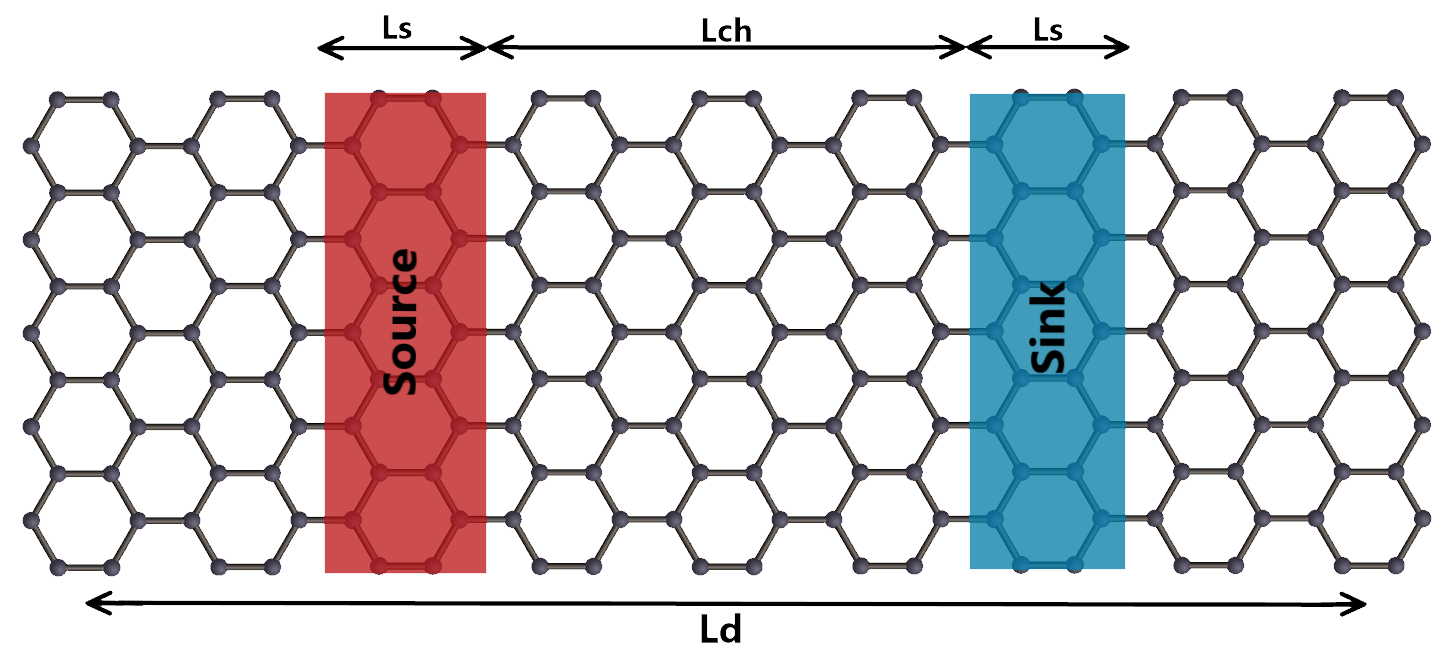
where $V$ is the sample volume. In reciprocal space, $\Delta T(\vec{k},\eta)=\Theta(\vec{k},\eta)P(\vec{k},\eta)$. We apply our analysis to graphene, depicted in Fig. 1.

Because graphene is a two-dimensional crystal, the vectors $\vec{r}$ and $\vec{k}$ are two-dimensional. Because the heat source and sink are parallel to the $y$ axis, the relevant wavevector is $\vec{k}=(k_{x},0)$. Heat current density $\vec{J}_{\rm 2D}$ has units W/m; the more familiar unit in 3D is W/m². Thermal conductivity in 2D has units W/K; in order to compare with 3D, it is conventional to choose the somewhat arbitrary “thickness” for graphene to be $h=3.4$ Å. This paper uses 3D units for current density $J=J_{\rm 2D}/h$, input power $P=P_{\rm 2D}/h$, energy density $U=U_{\rm 2D}/h$, and specific heat $C=C_{\rm 2D}/h$. Then $\kappa$ has conventional units W/mK, and $\Theta$ has units Km³/W.

The measured thermal conductivity of graphene (in 3D units) is reported to lie in the range of 2600 to 5300 W/mK at room temperature [28, 29]. The theoretical thermal conductivity of pristine infinite-size graphene at room temperature is reported in the range of 2800-4300 W/mK [13, 19, 30]. In devices smaller than mean free paths $\Lambda_{Q}$ of important phonons, the measured heat current divided by an approximate measurement of temperature gradient gives an “effective thermal conductivity” ($\kappa_{\rm eff}$) of smaller value. For phonons with bulk $\Lambda_{Q}=|v_{Qx}|\tau_{Q}$ ($\vec{v}_{Q}$ is phonon group velocity) greater than device size $L$, the contribution to $\kappa_{\rm eff}$ is reduced from $C_{Q}|v_{Q,x}|\Lambda_{Q}$ to $C_{Q}|v_{Qx}|L$, where $C_{Q}$ is the contribution of mode $Q$ to the specific heat. We will describe this effect using the thermal distributor function [23].

Under the assumptions of well-defined quasiparticles, the PBE in a crystalline solid is:

$$\frac{dN_{Q}}{dt}=\left(\frac{\partial N_{Q}}{\partial t}\right)_{\rm drift}+\left(\frac{\partial N_{Q}}{\partial t}\right)_{\rm scat}+\left(\frac{\partial N_{Q}}{\partial t}\right)_{\rm ext},$$

(8)

The first term on the right-hand side of Eq. 8 is the change of $N_{Q}$ caused by phonon drift in the distribution gradient:

$$\left(\frac{\partial N_{Q}}{\partial t}\right)_{\rm drift}=-\vec{v_{Q}}.\vec{\nabla}_{\vec{r}}N_{Q}$$

(9)

where $\vec{\nabla}_{\vec{r}}$ is the spatial gradient. The second term in Eq. 8 contains all scattering processes in the crystal. The term from anharmonic three-phonon scatterings ($Q\rightarrow Q^{\prime}+Q^{\prime\prime},Q+Q^{\prime}\rightarrow Q^{\prime\prime}$) can be found from the Fermi golden rule [31]:

$$\begin{split}\left(\frac{\partial N_{Q}}{\partial t}\right)_{\rm scat}&=\frac{\pi\hbar}{16N_{q}}\sum_{Q^{\prime}Q^{\prime\prime}}\left|V_{QQ^{\prime}Q^{\prime\prime}}\right|^{2}\\ &\frac{1}{2}\bigg{\{}N_{Q}(N_{Q^{\prime}}+1)(N_{Q^{\prime\prime}}+1)-(N_{Q}+1)N_{Q^{\prime}}N_{Q^{\prime\prime}}\bigg{\}}\delta(\omega_{Q}-\omega_{Q^{\prime}}-\omega_{Q^{\prime\prime}})\\ &+\bigg{\{}N_{Q}N_{Q^{\prime}}(N_{Q^{\prime\prime}}+1)-(N_{Q}+1)(N_{Q^{\prime}}+1)N_{Q^{\prime\prime}}\bigg{\}}\delta(\omega_{Q}+\omega_{Q^{\prime}}-\omega_{Q^{\prime\prime}}),\end{split}$$

(10)

where $\omega_{Q}$ is the phonon frequency and $N_{q}$ is a number of wavevectors in the Brillouin zone ¹¹1In the simulations, we use $N_{q}=120\times 120$ $q$-points to sample the Brillouin zone of graphene and for delta functions in Eq. (10) we use Gaussian broadening function $\delta(x)=\exp{-(x/\sigma)^{2}}/\sqrt{\pi}\sigma$ with $\hbar\sigma=0.9$ meV.. $V_{QQ^{\prime}Q^{\prime\prime}}$ is the matrix element of the three-phonon process, given by,

$$\begin{split}V_{QQ^{\prime}Q^{\prime\prime}}=\sum_{MLnml}\sum_{\alpha\beta\gamma}\frac{\epsilon_{Q}^{n\alpha}\epsilon_{Q^{\prime}}^{m\beta}\epsilon_{Q^{\prime\prime}}^{l\gamma}}{\sqrt{M_{\rm c}^{3}\omega_{Q}\omega_{Q^{\prime}}\omega_{Q^{\prime\prime}}}}\Psi_{\alpha\beta\gamma}(0n,Mm,Ll)e^{i\bm{q^{\prime}.R_{M}}}e^{i\bm{q^{\prime\prime}.R_{L}}}\delta(q+q^{\prime}+q^{\prime\prime},G),\end{split}$$

(11)

where $\Psi_{\alpha\beta\gamma}(0n,Mm,Ll)$ is the third derivative of the crystal potential by displacements of atoms in positions $(n,m,l)$ inside the unit cells $(0,M,L)$. The supercell with index $0$ is the central unit cell. $\epsilon_{Q}^{n\alpha}$ is the $\alpha^{\rm th}$ Cartesian component of the polarization vector of mode $Q$ at atom $n$, and $M_{\rm c}$ is the mass of a carbon atom. The Kronecker delta ensures the conservation of the lattice momentum, where $G$ is a reciprocal lattice vector. The local equilibrium phonon population $n_{Q}=n_{Q}(T(\vec{r},t))$ depends implicitly on the space and time through its explicit dependence on the temperature $T(\vec{r},t)$. For small deviations from equilibrium, expand the phonon population $N_{Q}$ as in Eq. 3 to first order in $\phi_{Q}$. The anharmonic scattering matrix $\hat{S}$ (Eq. 4) then has diagonal and off-diagonal elements,

	$\displaystyle S_{QQ}$	$\displaystyle=$	$\displaystyle 1/\tau_{Q}=2\pi\hbar\sum_{Q^{\prime}Q^{\prime\prime}}\left|V_{QQ^{\prime}Q^{\prime\prime}}\right|^{2}$
			$\displaystyle\bigg{\{}\frac{(n_{Q}^{0}+1)n_{Q^{\prime}}^{0}n_{Q^{\prime\prime}}^{0}}{2}\delta(\omega_{Q}-\omega_{Q^{\prime}}-\omega_{Q^{\prime\prime}})+n_{Q}^{0}n_{Q^{\prime}}^{0}(n_{Q^{\prime\prime}}^{0}+1)\delta(\omega_{Q}+\omega_{Q^{\prime}}-\omega_{Q^{\prime\prime}})\bigg{\}}$
	$\displaystyle S_{QQ^{\prime}}$	$\displaystyle=$	$\displaystyle 2\pi\hbar\sum_{Q^{\prime\prime}}\left|V_{QQ^{\prime}Q^{\prime\prime}}\right|^{2}\bigg{\{}n_{Q}^{0}n_{Q^{\prime}}^{0}(n_{Q^{\prime\prime}}^{0}+1)\delta(\omega_{Q}+\omega_{Q^{\prime}}-\omega_{Q^{\prime\prime}})$		(12)
			$\displaystyle-(n_{Q}^{0}+1)n_{Q^{\prime}}^{0}n_{Q^{\prime\prime}}^{0}\delta(\omega_{Q}-\omega_{Q^{\prime}}-\omega_{Q^{\prime\prime}})-n_{Q}^{0}(n_{Q^{\prime}}^{0}+1)n_{Q^{\prime\prime}}^{0}\delta(\omega_{Q}-\omega_{Q^{\prime}}+\omega_{Q^{\prime\prime}})\bigg{\}}$

This version of the scattering matrix is real-symmetric ($S_{QQ^{\prime}}=S_{Q^{\prime}Q}$) i.e. Hermitian. Each collision conserves phonon energy, which is assured by

$$S_{QQ}\omega_{Q}+\sum_{Q^{\prime},Q^{\prime}\neq Q}S_{QQ^{\prime}}\omega_{Q^{\prime}}=0,\ {\rm or}\ \hat{S}|\omega\rangle=0.$$

(13)

The mode frequency $\omega_{Q}=\langle Q|\omega\rangle$ is an eigenvector, in fact, the only “null eigenvector”, of the linearized Hermitian scattering operator $S_{QQ^{\prime}}=\langle Q|\hat{S}|Q^{\prime}\rangle$.

The last term in Eq. (8) models external heat sources and sinks. The form is usually [33, 34]

$$\left(\frac{\partial N_{Q}}{\partial t}\right)_{\rm ext}=\frac{P_{Q}(\vec{r},t)}{C}\frac{dn_{Q}}{dT},$$

(14)

The heat source/sink $P$, its geometry $(\vec{r},t)$, and its spectral distribution $Q$ determine whether the heat transport is quasiballistic or diffusive. We use the simplest version where $P_{Q}=P$ is independent of $Q$ [35, 36, 8, 34],

$$\left(\frac{\partial N_{Q}}{\partial t}\right)_{\rm ext}=\frac{P}{C}\frac{dn_{Q}}{dT},$$

(15)

where $P$ is the heat power added per unit volume of the system. Each mode gets the same boost $\Delta T$ from $P(\vec{r},t)$. Detailed knowledge of source and sink would cause a $Q$-dependence of $P$ [23, 37], but missing this knowledge, $P_{Q}=P$ is a sensible guess.

In vector-space notation, the LPBE, Eq. 8, is

$$\frac{\partial}{\partial t}[|n\rangle+|n^{0}(n^{0}+1)\phi\rangle]=-\vec{v_{Q}}\vec{\nabla}_{\vec{r}}[|n\rangle+|n^{0}(n^{0}+1)\phi\rangle]-\hat{S}|\phi\rangle+\frac{P(\vec{r},t)}{C}|\frac{dn}{dT}\rangle.$$

(16)

In this notation, the kets (like $|n\rangle$) are vectors in the space of phonon modes, with components $\langle Q|n\rangle=n_{Q}$. The solution $\phi_{Q}(\vec{r},t)$ is found from its Fourier $(\vec{k},\eta)$ representation,

$$\phi_{Q}(\vec{r},t)=\frac{1}{2\pi}\int_{-\infty}^{\infty}d\eta e^{-i\eta t}\sum_{\vec{k}}e^{i\vec{k}\cdot\vec{r}}\phi(\vec{k},\eta).$$

(17)

The temperature deviation $\Delta T(\vec{r},t)$ and the power input $P(\vec{r},t)$ are also transformed to Fourier space. To simplify the algebra, define a vector $|X\rangle$ and an operator $\hat{W}$.

$$|X\rangle\equiv|n^{0}(n^{0}+1)\hbar\omega\rangle$$

(18)

$$\hat{W}\equiv\hat{S}+i(\vec{k}\cdot\hat{\vec{v}}-\eta\hat{1})\hat{n}^{0}(\hat{n}^{0}+\hat{1})$$

(19)

where $\hat{\vec{v}}$ and $\hat{n}^{0}$ are diagonal in $Q$ space (i.e. $\langle Q|\hat{n}^{0}|Q^{\prime}\rangle=n_{Q}^{0}\delta(Q,Q^{\prime})=\langle Q|n^{0}\rangle\delta(Q,Q^{\prime})$). The LPBE in Fourier space is

$$\begin{split}\hat{W}|\phi\rangle=\frac{1}{k_{B}T^{2}}&\Big{[}-i(\vec{k}\cdot\hat{\vec{v}}-\eta\hat{1})\Delta T(\vec{k},\eta)+\\ &\frac{P(\vec{k},\eta)}{C}\hat{1}\Big{]}|X\rangle\end{split}$$

(20)

Quasiparticle heat transport in solids can be roughly categorized into three regimes: ballistic, quasi-ballistic, and diffusive. In the diffusive regime, where Fourier’s law applies, the channel length of the heat conductors is much longer than the MFPs; phonons experience multiple scattering events, so that a local equilibrium is established, with a temperature gradient that is constant everywhere except in the small region close to heat sources and sinks. Thermal transport is ballistic when the channel length is comparable to or less than phonon MFPs. In this case, thermal energy is mainly dissipated near the heat sources. The temperature gradient becomes thermally inhomogeneous, and heat current has a non-local relation to temperature. When the channel length is similar to the averaged phonon MFP, some phonons travel ballistically and others diffusely; heat transfer is “quasi-ballistic”. The wide range of phonon MFPs in graphene  [38] makes it hard to differentiate transport regimes. Moreover, the heat transport regime in a given device is temperature-dependent since the phonon MFPs depend on temperature.

The thermal distributor $\Theta(\vec{r})$, Eq. 6, simplifies the description of heat transport in different regimes. The spatial variation of temperature is given by

$$T(\vec{r})=\sum_{\vec{k}}T(\vec{k})e^{i\vec{k}\cdot\vec{r}}=\sum_{\vec{k}}\Theta(\vec{k})P(\vec{k})e^{i\vec{k}\cdot\vec{r}}.$$

(30)

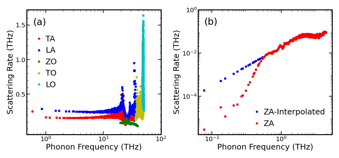
The Fourier transform $\Theta(\vec{k})$ is related to the non-local generalization of the bulk thermal conductivity $\kappa_{\rm bulk}={\rm lim}_{\vec{k}\rightarrow 0}\kappa(\vec{k})$ by Eq. 26. First, we calculate LPBE and RTA versions of $\Theta(\vec{k})$ of graphene from Eq. (27) and Eq. (29), using the modified Tersoff potential, with the parameters given in ref. 39, to model the crystal potential. The scattering rates are shown in Fig. 2 at $T=300$ K.

Note that there are numerical challenges in calculating the scattering rates of phonons using the Gaussian broadening [40]. Following Ref. [13, 31], we apply linear interpolation of the ZA scattering rates with phonon energy, as shown by the blue circles for phonon energies below 0.3 THz in Fig. 2b. This linear scaling is explained by noting that the bending energy is given by $E_{b}=\int d^{2}r\kappa_{b}/(2R^{2})$, where $\kappa_{b}=2.1$ eV [41] is the bending stiffness, and $R$ is the radius of curvature given by $1/R=d^{2}z/dx^{2}$. Applying the Bloch theorem for a discrete atomic model with a lattice constant $a$, one can show that bending energy for mode $q$ is given by $E_{b}=8\kappa_{b}A_{c}z_{q}^{2}\sin^{4}(qa/2)/a^{4}\approx A_{c}\kappa_{b}z_{q}^{2}q^{4}/2$, where $A_{c}$ is the area per atom. By comparing it to the harmonic oscillator potential energy $m\omega_{q}^{2}z_{q}^{2}/2$, one can obtain the expected result for flexural phonon frequency: $\omega_{q}=q^{2}\sqrt{\kappa_{b}A_{c}/m}$. The third order anharmonicity can be introduced by coupling the ZA mode to an LA mode by modifying the bending stiffness $\kappa_{b}=\kappa_{b0}-\alpha_{b}(x_{i+1}-x_{i-1})$. After applying the Bloch theorem, the third-order anharmonic potential for mode $q$ in the small $q$-limit becomes $H_{3}=\sum_{q_{1}}i\alpha_{b}A_{c}z_{q}z_{q_{1}}x_{-q-q_{1}}q^{2}q_{1}^{2}(q+q_{1})a$. Using second-quantized amplitudes for the phonon displacements $z_{q}$ and $x_{q}$, one can show that $V_{qq_{1}}\sim q^{2}q_{1}^{2}(q+q_{1})(\omega_{q}^{ZA}\omega_{q_{1}}^{ZA}\omega_{q+q_{1}}^{LA})^{-1/2}$. The $q$-ZA phonon scattering with $q_{1}$-ZA phonon into an $(q+q_{1})$-LA phonon has a rate of $1/\tau^{ZA}_{q}\sim\sum_{q_{1}}|V_{q,q_{1}}|^{2}n^{0,ZA}_{q_{1}}n^{0,LA}_{q+q_{1}}\delta(\omega^{ZA}_{q}+\omega^{ZA}_{q_{1}}-\omega^{LA}_{q+q_{1}})$. The $\delta$-function ensures that $q_{1}\sim v_{s}\sqrt{m/(\kappa_{b}A_{c})}$, where $v_{s}$ is the sound velocity. Therefore, the interpolation function $1/\tau^{ZA}_{q}\sim q^{2}\sim\omega^{ZA}_{q}$ used in Fig. 2b can be justified.

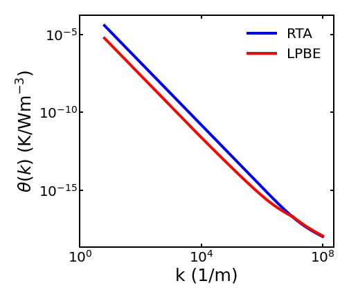
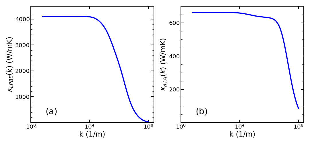
Fig. 3 shows the calculated $\Theta(k)$ for graphene using LPBE and RTA approximations. The width of the sample is much broader than the MFP; this allows a one-dimensional treatment. The spatial variation $\vec{r}=(x,0)$ is only along $\hat{x}$, parallel to the channel, so the spatial Fourier variable is $\vec{k}=(k,0)$. The spatial resolution of $T(x)$ at small distances $x$ requires values of $\Theta(k)$ at correspondingly large $k\sim 2\pi/x$ (see Eq. 30). The range of $k$ in Fig. 3 corresponds to distances from a few nanometers to a meter-long channel length. A lower limit of the length scale is imposed by the validity of the quasiparticle picture of phonons used in the PBE formalism  [26]. Note that the thermal distributor diverges for both LPBE and RTA solutions when $k\to 0$. According to Eq. (26), for a finite thermal conductivity in a diffusive regime, $\Theta(k)$ must diverge in $k\to 0$ limit as $\Theta(k)\sim\frac{1}{k^{2}}$. Curve-fitting shows that the calculated $\Theta(k)$ for both versions agrees with $\frac{1}{k^{2}}$ very accurately in the small $k$ limit, namely:

$$\begin{split}&\Theta_{LBPE}(k)=\frac{2.4\times 10^{-4}\ {\rm Km/W}}{k^{2}}\\ &\Theta_{RTA}(k)=\frac{1.51\times 10^{-3}\ {\rm Km/W}}{k^{2}}\end{split}$$

(31)

Using Eq. (26), this corresponds to bulk thermal conductivities 4145 W/mK and 662 W/mK for LPBE and RTA, respectively. The large discrepancy between LPBE and RTA values of thermal conductivities of graphene has been noticed previously [13].

The thermal conductivities evaluated according to Eq. (25) for LPBE and Eqs. 26, 29 for RTA are shown in Fig. 4. The sharp fall-off of the thermal conductivity in Fig. 4 indicates the ballistic-to-diffusive crossover; it happens at larger $k$, and, therefore, smaller characteristic lengths in the RTA treatment than in the correct LPBE treatment.

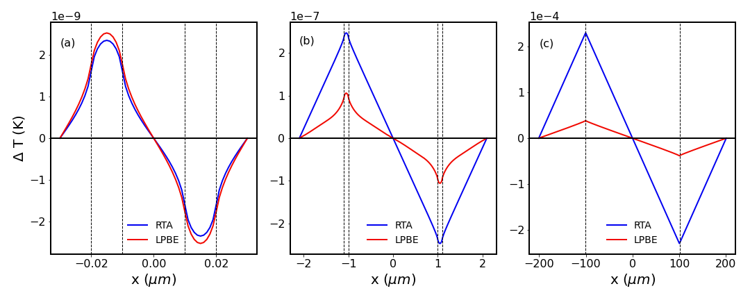
Now we discuss thermal conduction in the geometry of Fig. 1 using the PBE to evaluate the thermal distributor. We can calculate the temperature profile for any pattern of heat input and removal from this response function, provided the graphene sample has one-dimensional periodicity. Energy conservation requires $dJ/dx=-P(x)$. Steady-state ($\eta=0$) requires equal external heat addition and removal. $L_{\rm ch}$ is the length of the channel between the two heat reservoirs, source and sink; each of length $L_{\rm s}$. For simplicity, our heat input has odd symmetry ($P(-x)=-P(x)$) around $x=0$, so $J$ is even in $x$. The period of the supercell is $L_{d}=2(L_{\rm ch}+L_{\rm s})$, which determines the shortest non-zero wavevector i.e. $k_{min}=2\pi/L_{d}$. A large $L_{d}$ value allows a fine Fourier mesh to describe nanoscale physics, such as the ballistic-to-diffusive crossover. Our reservoirs are ideal thermal baths, with zero interfacial thermal resistance between the channel and reservoirs. Note that experimental thermal conductivity measurements are often done using periodic structures such as periodic metallic gratings or transient thermal gratings  [42, 43]. Our periodic geometry of Fig. 1 works for both periodic structures and single-channel devices. In the latter case, it is necessary to make $L_{\rm s}$ larger than phonon MFPs.

Figure 1 shows how heat insertion and removal $P(x)$ is distributed uniformly (with magnitude $P_{0}$) over lengths $L_{\rm s}$ on either side of the sample (or channel) of length $L_{\rm ch}$. Energy conservation $dJ/dx=P$ then gives heat current density $J=P_{0}L_{\rm s}/2$ in the channels. Figure 5 shows the resulting $\Delta T$ profiles in three devices with channel lengths spanning from ballistic to diffusive regimes. In the ballistic device, Fig. 5a, both $\Theta_{RTA}$ and $\Theta_{LBTE}$ predict similar values for temperature profiles in the channel and in the source/sink reservoirs. This behavior can be understood from the two thermal distributors being similar in magnitude in the large $k$-limit, as shown in Fig. 3. The temperature profile of Fig. 5a clearly shows the source regions are hotter than the channel, which is a characteristic of non-diffusive thermal transport [34, 33, 44]. The long MFP phonons (ZA phonons) dissipate the thermal energy in the source regions while flying in the channel ballistically. As a result, the temperature is higher in the heat region. This observation manifests the nonlocal effect.

For the larger channel lengths in Fig. 5b and 5c, RTA predictions for the temperature are significantly higher than LPBE predictions in agreement with Fig. 3 which shows that at smaller $k$ (corresponding to larger distances) $\Theta_{RTA}$ is greater than $\Theta_{LPBE}(k)$. In the quasi-ballistic regime of Fig. 5b, there is significant non-linearity near the heat source/sink. Although in this regime both long and short MFP phonons contribute to thermal transport, the share of thermal energy carried by short MFP phonons is almost negligible.

Non-local heat transport is often described by an “effective thermal conductivity” $\kappa_{\rm eff}$. The definition varies depending on the experiment. For example, experimental studies such as time-domain thermoreflectance [45] measure the transient temperature response to a heat pulse. This can be used to extract $\kappa_{\rm eff}$ [42]. Many theoretical studies also have applied a similar procedure.

For our steady-state thermal transport computations, there are three sensible definitions of $\kappa_{\rm eff}$, shown in table 1. The first of these defines $\kappa_{\rm eff}$ by applying Fourier’s law at the middle of the channel where the curvature of $\Delta T(x)$ is zero. This resembles Fourier’s law in thermally homogeneous structures. We note that in the fully diffusive regime, when both $L_{\rm s}$ and $L_{\rm ch}$ are larger than the MFPs, the $\kappa_{\rm eff,mp}$ and $\kappa_{\rm eff,ch}$ values coincide, and the temperature drop in the channel is $\Delta T_{\rm ch}=J_{0}L_{\rm ch}/\kappa_{\rm eff,mp}$. In this limit, the temperature drop under the contact is equal to $J_{0}L_{\rm s}/(4\kappa_{\rm eff,mp})$, because current $J(x)$ varies linearly with distance from the middle of the contact. Therefore, the maximum temperature variation across the unit cell equals $\Delta T_{\rm max}=\Delta T_{\rm ch}+J_{0}L_{\rm s}/(2\kappa_{\rm eff,mp})$ and effective thermal conductivity $\kappa_{\rm eff,min}=J_{0}(L_{\rm ch}+L_{\rm s})/\Delta T_{\rm max}=\kappa_{\rm eff,mp}(L_{\rm ch}+L_{\rm s})/(L_{\rm ch}+L_{\rm s}/2)$. As can be seen from table 1, the device geometry in Fig. 5c approaches the diffusive limit. However, one should note the fully diffusive limit relationship between $\kappa_{\rm eff,min}$ and $\kappa_{\rm eff,mp}$ is not realized in the devices we considered.

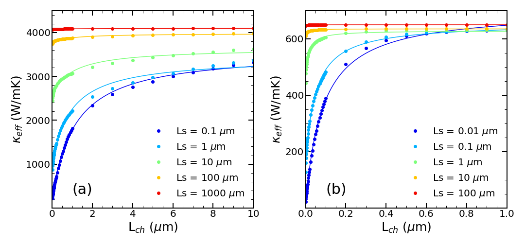
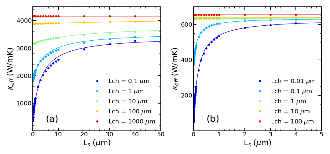
The $\kappa_{\rm eff,mp}$ definition is plotted in Fig. 6 and 7, for both LPBE and RTA versions of the thermal distributor, as a function of the source length and channel length, respectively. When the chosen length $L_{\rm ch}$ in Fig. 6 (or $L_{\rm s}$ in Fig. 7) has a value less than the diffusive length scale ($\sim 1-3\>\mu$m for LPBE and $\sim 100-200\>$ nm for RTA), $\kappa_{\rm eff,mp}$ decreases with decreasing periodicity due to suppression of the ballistic phonon contribution to the heat transport. At large values of $L_{\rm ch}$, thermal conductivity saturates and approaches the diffusive limit when both $L_{\rm ch}$ and $L_{\rm s}$ are large.

Similarly, Fig. 7 shows that $\kappa_{\rm eff,mp}$ saturates with increasing $L_{\rm s}$ and reaches the diffusive limit value at large $L_{\rm ch}$. For small $L_{\rm ch}$ values, the $\kappa_{\rm eff,mp}$ dependence on $L_{\rm s}$ shows ballistic to diffusive crossover as in Fig. 6. Those dependencies happen because of superposing interaction of ballistic phonons in the ballistic channels and recovery of diffusive-like thermal transport. This phenomenon shows the deterministic role of the geometry of the heat source and has already been observed experimentally  [43, 46].

To quantify our results in Fig. 6 and 7, we fit our $\kappa_{\rm eff,mp}$ to the phenomenological ballistic-to-diffusive crossover equations used to describe electrical transport [47]:

	$\displaystyle\kappa_{\rm eff,a}$	$\displaystyle=$	$\displaystyle\kappa_{0}+(\kappa_{\rm dif}-\kappa_{0})\frac{L_{\rm ch}}{L_{\rm ch}+\lambda}\$		(32)
	$\displaystyle\kappa_{\rm eff,b}$	$\displaystyle=$	$\displaystyle\kappa_{0}+(\kappa_{\rm dif}-\kappa_{0})\frac{L_{\rm s}}{L_{\rm s}+\lambda}$		(33)

where $\kappa_{\rm dif}$ is thermal conductivity in the diffusive regime. From the best fits, we find a characteristic length scale $\lambda\sim 1$ $\mu$m ($\sim 90$ nm) for the LPBE (RTA) solution using fits of $\kappa_{\rm eff,a}$ versus $L_{\rm ch}$, and $\lambda\sim 3$ $\mu$m ($\sim 200$ nm) for LPBE (RTA) solution using fits of $\kappa_{\rm eff,b}$ versus $L_{\rm s}$. The value of $\kappa_{0}$ approaches zero only when both $L_{\rm s}$ and $L_{\rm ch}$ are small, as discussed above. Those estimates for the characteristic crossover length scales are consistent with the $k$-dependences of thermal conductivity in Fig. 4. Using a characteristic value of $k_{0}$, when thermal conductivity drops by a factor of two in Fig. 4, we find $2\pi/k_{0}\sim 5$ $\mu$m for LPBE and $2\pi/k_{0}\sim 300$ nm for RTA. Finally, we can estimate an average phonon MFP using the standard expression for thermal conductivity in 2D: $\kappa=Cv\lambda_{\rm ph}/2$, where the heat capacity is $C\times h=4.5\times 10^{-4}{\rm J/Km}^{2}$ (calculated at $T=300$ K) and $v$ is an averaged phonon velocity. Using the velocity of the ZA parabolic band at room temperature $v\approx 10$ km/s, we obtain $\lambda_{\rm ph}=625$ nm for LPBE and $\lambda_{\rm ph}=100$ nm for RTA, consistent with the above estimates for the diffusive to ballistic crossover length scales.

Steady microscale addition and removal of heat energy, together with a scattering of heat carriers, leads to carrier distributions $N$ centered around local equilibrium $n$ with a local temperature $T(x)$. The thermal distributor $\Theta(k)$ contains all relevant information about thermal transport in all the regimes. By computing the thermal distributor $\Theta(k)$ of graphene from the PBE with correct inversion using the full scattering operator, we investigated thermal transport at submicron length scales. At long length scales, heat transport occurs with constant temperature gradients. Non-local effects (where $\nabla T$ varies with $x$) are seen at length scales of the order of or less than mean free paths of phonons. Details of the geometrical structure of the device and heat sources and sinks cause the inhomogeneous temperature profile $T(x)$. The long-wavelength phonons are forcefully scattered in the source and sink regions while flying the channel without appreciable scatterings with other phonons. This causes local $\Delta T(x)$ to be higher near the source/sink. This is often ascribed to the suppression of heat transport by phonons with long mean free paths. The RTA contains these effects but, especially in graphene, overestimates the temperature inhomogeneity needed to drive a heat current.

We acknowledge support from the Vice President for Research and Economic Development (VPRED), SUNY Research Seed Grant Program, and the Center for Computational Research at the University at Buffalo [48].

References

- Peierls [1929] R. Peierls, Zur kinetischen Theorie der Wärmeleitung in Kristallen, Annalen der Physik 395, 1055 (1929).
- Simons [1960] S. Simons, The Boltzmann equation for a bounded medium I. General theory, Phil. Trans. Roy. Soc. London. Series A, Math. Phys. Sci. 253, 137 (1960).
- Levinson [1980] Y. Levinson, Nonlocal phonon heat transfer, Sol. State Commun. 36, 73 (1980).
- Mahan and Claro [1988] G. Mahan and F. Claro, Nonlocal theory of thermal conductivity, Phys. Rev. B 38, 1963 (1988).
- Majumdar [1993] A. Majumdar, Microscale heat conduction in dielectric thin films, ASME J. Heat Transfer 115, 7 (1993).
- Chen [2005] G. Chen, Nanoscale energy transport and conversion: a parallel treatment of electrons, molecules, phonons, and photons (Oxford University Press, 2005).
- Ordonez-Miranda et al. [2011] J. Ordonez-Miranda, R. Yang, and J. Alvarado-Gil, A constitutive equation for nano-to-macro-scale heat conduction based on the Boltzmann transport equation, J. Appl. Phys. 109, 084319 (2011).
- Allen and Perebeinos [2018] P. B. Allen and V. Perebeinos, Temperature in a Peierls-Boltzmann treatment of nonlocal phonon heat transport, Phys. Rev. B 98, 085427 (2018).
- Hua et al. [2019] C. Hua, L. Lindsay, X. Chen, and A. J. Minnich, Generalized Fourier’s law for nondiffusive thermal transport: Theory and experiment, Phys. Rev. B 100, 085203 (2019).
- Hua and Lindsay [2020] C. Hua and L. Lindsay, Space-time dependent thermal conductivity in nonlocal thermal transport, Phys. Rev. B 102, 104310 (2020).
- Simoncelli et al. [2020] M. Simoncelli, N. Marzari, and A. Cepellotti, Generalization of Fourier’s law into viscous heat equations, Phys. Rev. X 10, 011019 (2020).
- Srivastava [1990] G. P. Srivastava, The physics of phonons (Routledge, 1990).
- Lindsay et al. [2014] L. Lindsay, W. Li, J. Carrete, N. Mingo, D. Broido, and T. Reinecke, Phonon thermal transport in strained and unstrained graphene from first principles, Phys. Rev. B 89, 155426 (2014).
- Lindsay [2016] L. Lindsay, First principles Peierls-Boltzmann phonon thermal transport: a topical review, Nanoscale and Microscale Thermophysical Engineering 20, 67 (2016).
- McGaughey et al. [2019] A. J. H. McGaughey, A. Jain, H.-Y. Kim, and B. Fu, Phonon properties and thermal conductivity from first principles, lattice dynamics, and the Boltzmann transport equation, J. App. Phys. 125, 011101 (2019).
- Cepellotti and Marzari [2016] A. Cepellotti and N. Marzari, Thermal transport in crystals as a kinetic theory of relaxons, Phys. Rev. X 6, 041013 (2016).
- Cepellotti and Marzari [2017] A. Cepellotti and N. Marzari, Transport waves as crystal excitations, Phys. Rev. Mat. 1, 045406 (2017).
- Fugallo et al. [2013] G. Fugallo, M. Lazzeri, L. Paulatto, and F. Mauri, Ab initio variational approach for evaluating lattice thermal conductivity, Phys. Rev. B 88, 045430 (2013).
- Fugallo et al. [2014] G. Fugallo, A. Cepellotti, L. Paulatto, M. Lazzeri, N. Marzari, and F. Mauri, Thermal conductivity of graphene and graphite: collective excitations and mean free paths, Nano letters 14, 6109 (2014).
- Li et al. [2014] W. Li, J. Carrete, N. A. Katcho, and N. Mingo, ShengBTE: A solver of the Boltzmann transport equation for phonons, Comp. Phys. Commun. 185, 1747 (2014).
- Chernatynskiy and Phillpot [2015] A. Chernatynskiy and S. R. Phillpot, Phonon transport simulator (PhonTS), Comp. Phys. Commun. 192, 196 (2015).
- Carrete et al. [2017] J. Carrete, B. Vermeersch, A. Katre, A. van Roekeghem, T. Wang, G. K. H. Madsen, and N. Mingo, almaBTE: A solver of the space–time dependent Boltzmann transport equation for phonons in structured materials, Comp. Phys. Commun. 220, 351 (2017).
- Hua and Minnich [2014] C. Hua and A. J. Minnich, Analytical Green’s function of the multidimensional frequency-dependent phonon Boltzmann equation, Phys. Rev. B 90, 214306 (2014).
- Zeng and Chen [2014] L. Zeng and G. Chen, Disparate quasiballistic heat conduction regimes from periodic heat sources on a substrate, J. Appl. Phys. 116, 064307 (2014).
- Collins et al. [2013] K. C. Collins, A. A. Maznev, Z. Tian, K. Esfarjani, K. A. Nelson, and G. Chen, Non-diffusive relaxation of a transient thermal grating analyzed with the Boltzmann transport equation, J. Appl. Phys. 114, 104302 (2013).
- Allen [2018] P. B. Allen, Analysis of nonlocal phonon thermal conductivity simulations showing the ballistic to diffusive crossover, Phys. Rev. B 97, 134307 (2018).
- Chiloyan et al. [2021] V. Chiloyan, S. Huberman, Z. Ding, J. Mendoza, A. A. Maznev, K. A. Nelson, and G. Chen, Green’s functions of the boltzmann transport equation with the full scattering matrix for phonon nanoscale transport beyond the relaxation-time approximation, Physical Review B 104, 245424 (2021).
- Balandin et al. [2008] A. A. Balandin, S. Ghosh, W. Bao, I. Calizo, D. Teweldebrhan, F. Miao, and C. N. Lau, Superior thermal conductivity of single-layer graphene, Nano letters 8, 902 (2008).
- Chen et al. [2011] S. Chen, A. L. Moore, W. Cai, J. W. Suk, J. An, C. Mishra, C. Amos, C. W. Magnuson, J. Kang, L. Shi, et al., Raman measurements of thermal transport in suspended monolayer graphene of variable sizes in vacuum and gaseous environments, ACS Nano 5, 321 (2011).
- Libbi et al. [2020] F. Libbi, N. Bonini, and N. Marzari, Thermomechanical properties of honeycomb lattices from internal-coordinates potentials: the case of graphene and hexagonal boron nitride, 2D Materials 8, 015026 (2020).
- Bonini et al. [2012] N. Bonini, J. Garg, and N. Marzari, Acoustic phonon lifetimes and thermal transport in free-standing and strained graphene, Nano Letters 12, 2673 (2012).
- Note [1] In the simulations, we use -points to sample the Brillouin zone of graphene and for delta functions in Eq. (10) we use Gaussian broadening function with meV.
- Hua and Minnich [2018] C. Hua and A. J. Minnich, Heat dissipation in the quasiballistic regime studied using the boltzmann equation in the spatial frequency domain, Physical Review B 97, 014307 (2018).
- Chiloyan et al. [2020] V. Chiloyan, S. Huberman, A. A. Maznev, K. A. Nelson, and G. Chen, Thermal transport exceeding bulk heat conduction due to nonthermal micro/nanoscale phonon populations, Applied Physics Letters 116, 163102 (2020).
- Vermeersch and Shakouri [2014] B. Vermeersch and A. Shakouri, Nonlocality in microscale heat conduction, ArXiv e-prints (2014), arXiv:1412.6555v2 .
- Vermeersch et al. [2015] B. Vermeersch, J. Carrete, N. Mingo, and A. Shakouri, Superdiffusive heat conduction in semiconductor alloys. I. Theoretical foundations, Phys. Rev. B 91, 085202 (2015).
- Allen and Nghiem [2022] P. B. Allen and N. A. Nghiem, Nonlocal phonon heat transport seen in 1-d pulses, to be published, ArXiv e-prints (2022), arXiv:2106.00867v4 .
- Li and Lee [2019] X. Li and S. Lee, Crossover of ballistic, hydrodynamic, and diffusive phonon transport in suspended graphene, Phys. Rev. B 99, 085202 (2019).
- Lindsay and Broido [2010] L. Lindsay and D. A. Broido, Optimized Tersoff and Brenner empirical potential parameters for lattice dynamics and phonon thermal transport in carbon nanotubes and graphene, Phys. Rev. B 81, 205441 (2010).
- Gu et al. [2019] X. Gu, Z. Fan, H. Bao, and C. Y. Zhao, Revisiting phonon-phonon scattering in single-layer graphene, Phys. Rev. B 100, 064306 (2019).
- Perebeinos and Tersoff [2009] V. Perebeinos and J. Tersoff, Valence force model for phonons in graphene and carbon nanotubes, Phys. Rev. B 79, 241409 (2009).
- Johnson et al. [2013] J. A. Johnson, A. A. Maznev, J. Cuffe, J. K. Eliason, A. J. Minnich, T. Kehoe, C. M. S. Torres, G. Chen, and K. A. Nelson, Direct measurement of room-temperature nondiffusive thermal transport over micron distances in a silicon membrane, Phys. Rev. Lett. 110, 025901 (2013).
- Zeng et al. [2015] L. Zeng, K. C. Collins, Y. Hu, M. N. Luckyanova, A. A. Maznev, S. Huberman, V. Chiloyan, J. Zhou, X. Huang, K. A. Nelson, et al., Measuring phonon mean free path distributions by probing quasiballistic phonon transport in grating nanostructures, Sci. Rep. 5, 1 (2015).
- Li et al. [2019] Z. Li, S. Xiong, C. Sievers, Y. Hu, Z. Fan, N. Wei, H. Bao, S. Chen, D. Donadio, and T. Ala-Nissila, Influence of thermostatting on nonequilibrium molecular dynamics simulations of heat conduction in solids, The Journal of chemical physics 151, 234105 (2019).
- Cahill [2004] D. G. Cahill, Analysis of heat flow in layered structures for time-domain thermoreflectance, Rev. Sci. Instr. 75, 5119 (2004).
- Hoogeboom-Pot et al. [2015] K. M. Hoogeboom-Pot, J. N. Hernandez-Charpak, X. Gu, T. D. Frazer, E. H. Anderson, W. Chao, R. W. Falcone, R. Yang, M. M. Murnane, H. C. Kapteyn, et al., A new regime of nanoscale thermal transport: Collective diffusion increases dissipation efficiency, Proc. Nat. Acad. Sci. 112, 4846 (2015).
- Lundstrom [2000] M. Lundstrom, Fundamentals of Carrier Transport, 2nd ed. (Cambridge University Press, 2000).
- [48] Center for Computational Research, University at Buffalo, http://hdl.handle.net/10477/79221.