Non-Markovian channel from the reduced dynamics of coin in quantum walk
Abstract
The quantum channels with memory, known as non-Markovian channels, are of crucial importance for a realistic description of a variety of physical systems, and pave ways for new methods of decoherence control by manipulating the properties of environment such as its frequency spectrum. In this work, the reduced dynamics of coin in a discrete-time quantum walk is characterized as a non-Markovian quantum channel. A general formalism is sketched to extract the Kraus operators for a -step quantum walk. Non-Markovianity, in the sense of P-indivisibility of the reduced coin dynamics, is inferred from the non-monotonous behavior of distinguishably of two orthogonal states subjected to it. Further, we study various quantum information theoretic quantities of a qubit under the action of this channel, putting in perspective, the role such channels can play in various quantum information processing tasks.
I Introduction
The study of open quantum systems with memory has attracted lot of attention over last few years, since such systems describe a plethora of physical phenomena and also provide new ways to control various quantum features by engineering the system-environment interactions Breuer et al. (2002); Banerjee (2018). Several investigations on the role of structured environments and non-Markovianity in entanglement generation Huelga et al. (2012), quantum teleportation Laine et al. (2014), key distribution Vasile et al. (2011), quantum metrology Chin et al. (2012), quantum biology Thorwart et al. (2009), have suggested the advantage of non-Markovian quantum channels over Markovian ones.
Quantum walks (QWs) was conceived as a generalization of classical random walks with an anticipation of its potential in modeling the dynamics particle in quantum realm Riazanov (1958); Feynman (1986); Parthasarathy (1988); Meyer and Shakeel (2016); Wong and Meyer (2016); Aharonov et al. (1993). They describe the coherent evolution of a quantum particle, coin space coupled to the position space which in principle can be treated as an external environment. One-dimensional QWs involve a walker free to move in either direction along a straight line such that the direction for each step is decided by the outcome of a coin. However, it differs from its classical counterpart in the sense that the probability distribution of the quantum particle spreads quadratically faster in position space than the classical random walk due to interference. This feature makes QWs ideal candidate for development of quantum algorithms such as quantum search algorithms Shenvi et al. (2003); Krovi and Brun (2006). Ability to engineering the dynamics of the QWs has also allowed us to simulate and study quantum correlations Srikanth et al. (2010); Chandrashekar et al. (2012); Rao et al. (2011), quantum to classical transition Chandrashekar et al. (2007); Banerjee et al. (2008), memory effects and disorder Kumar et al. (2018), relativistic quantum effects Chandrashekar et al. (2010) and quantum games Chandrashekar and Banerjee (2011). Experimental implementation of QWs has been realized in various physical systems viz., in cold atoms Perets et al. (2008); Karski et al. (2009), photonic systems Peruzzo et al. (2010); Schreiber et al. (2010); Broome et al. (2010); Tamura et al. (2020); Kitagawa et al. (2012); Preiss et al. (2015); Côté et al. (2006). Recent studies have reported the circuit based implementation of QW Ryan et al. (2005); Qiang et al. (2016); Alderete et al. (2020). A scheme for implementing QW in Bose-Einstein condensates was presented in Chandrashekar (2006) and was recently implemented in momentum space Dadras et al. (2018). Possible applications of QWs in understanding the dynamics in biological systems have been reported in various works Hoyer et al. (2010); Mohseni et al. (2008); Rebentrost et al. (2009).
The QW can be discrete or continuous in time, accordingly known as Discrete Time Quantum Walk (DTQW) and Continuous Time Quantum Walk (CTQW). In this work, we confine ourselves to the former case. The DTQW was studied from the perspective of various facets of non-Markovian evolution, such as the disambiguation of contributions to non-Markovian backflow as well as the transition from quantum to classical random walks Kumar et al. (2018). The non-Markovian nature of coin dynamics in DTQW can be brought out by tracing over the position space Hinarejos et al. (2014). Henceforth, we will coin the term quantum walk noise (QWN) to describe the reduced dynamics on the coin space. In this work, we quantify this by developing the Kraus operators for the QWN, thereby characterizing the QW channel. The QWN was studied Kumar et al. (2018) in conjunction with an RTN Daffer et al. (2004); Van Kampen (1992) noise. The P-indivisibility Rivas et al. (2014); Breuer et al. (2016); Shrikant et al. (2019) of the QWN as well as the RTN suggested that the intermediate map of the full evolution could be not completely positive (NCP). Also, non-monotonic behavior under trace distance was indicated. This called for a careful consideration of the application of such non-Markovian noise channels to the DTQW protocol. A suggestion offered in Kumar et al. (2018) was that in contrast to the conventional application of the (Markovian) noise channel Chandrashekar et al. (2007); Banerjee et al. (2008) in the form of appropriate Kraus operators Banerjee (2018), after each application of the walk operation, in the present non-Markovian scenario, the Kraus operators are applied once after QW steps. This notion was implemented numerically. Here, making use of the developed Kraus operators of the QW channel, we quantify this notion. This, thus also serves the purpose of highlighting the implementation of non-Markovian noise channels to various QW protocols. We further characterize the QW channel by studying various information theoretic processes on it. Specifically, the interplay of purity of qubit state with the channel parameter as well as the state parameter is investigated. Further, the Holevo quantity, which characterizes the information about an input state that can be retrieved from the output of the channel, is studied.
The paper is organized as follows: In Sec. (II), the reduced coin dynamics is studied, sketching the formalism to extract the Kraus operators for a -step walk. Section (III) is devoted to a detailed investigation of various properties of QW channel, such as its non-Markovian nature in the sense of P-indivisibility in Sec. (III.1), the purity of states subjected to this channel in Sec. (III.2), and the Holevo quantity in Sec. (III.3). Conclusion of this work is presented in Sec. (IV).
II Reduced Dynamics of Coin
Let the initial state of coin and walker be and , respectively. The unitary operator , where and are the shift and coin operators, respectively, governs the time evolution of the combined state . The state after steps is given by Chandrashekar (2010)
| (1) |
Here, , , and are the corresponding density matrices. Further, the coin and shift operators are given by
| (2) |
The operator , and , are the left and right shift operators, respectively. The total unitary operator for steps becomes
Here, , , , and . The right hand side can be simplified using the binomial expansion Wyss (2017)
| (4) |
The second term arises due to the non-commutative nature of and , and can be simplified using the recurrence relation
| (5) |
Thus, the quantity vanishes if . From the definition of and , it follows
| (6) |
Using the definition of , it follows that , and is a zero matrix only for , , and , which correspond to the coin operator being identity.
Further simplification of the first term in Eq. (4) reads
| (7) |
For a walk of -steps, symmetric about , the number of values position can take is . Let the initial state of coin and walker be (with ) and , respectively. The possible position states are . We represent these states in computational basis as , , , respectively.
With this setting, we trace over the position degrees of freedom, using notation , and obtain
| (8) |
The Kraus operators are identified as , with .
| (9) |
In order to simplify the first term, we assume , i.e., the walker starts at , such that
| (10) |
Use has been made of , see the Appendix. The constraints and demand that and have same parity, i.e., for even (odd), is even (odd).
For a one step walk, , implies . From Eq. (5) , we have , leading to
| (11) |
These operators satisfy the completeness condition . Table (1) lists the Kraus operators for the reduced coin dynamics for a few steps of symmetric QW. One infers that,
-
1.
, where is the minor of the matrix .
-
2.
For coin parameter , , , and , with being the identity matrix.
 |
 |
| (a) | (b) |
 |
 |
| (c) | (d) |
The Kraus operators constitute a map connecting the input state to output . Let with , we have
| (12) |
Here, is the probability of obtaining in an -step walk. The form of and for some steps is given below
| (13) |
and
| (14) |
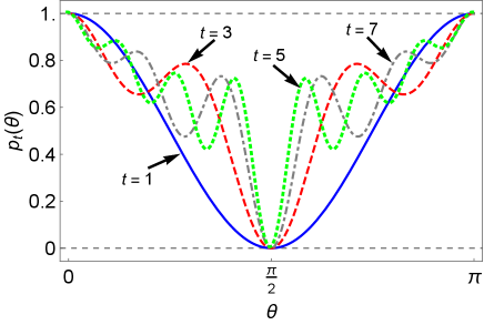
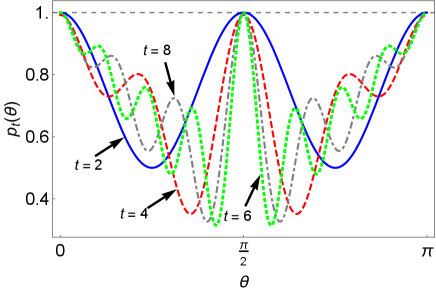
The probabilities are plotted in Fig. 1 (a)-(b) when , with respect to the coin parameter . The asymmetric behavior of the probabilities, with respect to even and odd number of steps, is observed at , where probabilities converge to one (zero) for even (odd) number of steps. The value of the coin parameter corresponds to the coin operator ( Eq. (2) ) , where is the Pauli operator.
| Steps | Kraus operators |
|---|---|
| 1 | |
| 2 | |
| 3 | |
| 4 |
There are other formulation of QW, like the split-step QW, where one breaks each step of walk into two half-step evolutions described by the unitary Singh et al. (2020). Here, is the unitary operator for the standard QW, defined in Eq. (1). The Kraus operators for some steps of the split-step QW are given in Table (2).
III Some properties of the QW channel
In this section, we characterize the non-Markovian QW channel comprising the reduced coin dynamics. We also study some quantum information theoretic quantities on it.
III.1 Non-Markovian dynamics
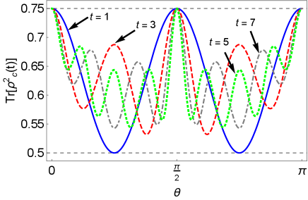
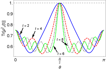
Non-Markovianity is a multifaceted phenomenon. Here, we restrict ourselves to the P-indivisibility form of non-Markovianity, that can be probed by using some state distinguishablity measure, such as trace distance, denoted by . Trace distance of states and is defined as , where are the eigenvalues of matrix . A departure from the monotonic behavior of implies P-indivisibility of the map , and hence non-Markovian dynamics. Consider two orthogonal states and , subjected to the QW channel for specific number of steps. For a one step walk, we have
| (15) |
Here, are the eigenvalues of and
| (16) |
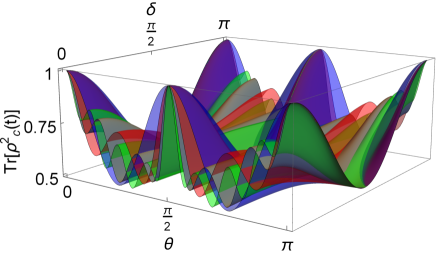
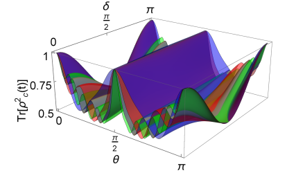
Similarly, we can compute the trace distance between and for arbitrary -number of steps, and is depicted in Fig. 3 (a). The fluctuating nature of the curves clearly bring out the P-indivisibility of the non-Markovian QW channel comprising the reduced coin dynamics.

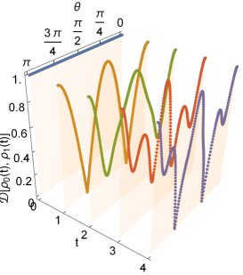 |
 |
 |
| (a) | (b) | (c) |
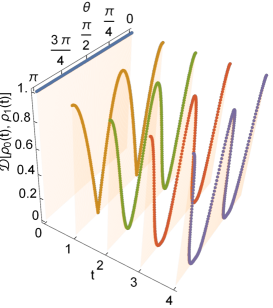
It is important to highlight the fact that for the case of non-Markovian processes, such as the P-indivisible case studied here, the concatenation of one step map times is not equivalent to operating with -step map, that is, , Fig. (2). This becomes clear when one computes the trace distance between and , which turns out to be a monotonically decreasing function in the former case
| (17) |
Unless , we have , therefore, converges to zero as increases, as shown in Fig. 3 (c).
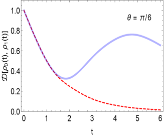
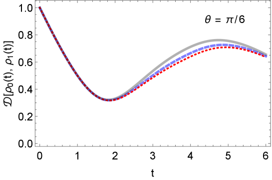
Discerning multiple non-Markovian effects: Quantum walks have been studied in the presence of various noise models, both Markovian and non-Markovian Kumar et al. (2018, 2018). It is important to mention here that the inferences drawn about the non-Markovian behavior in such cases must take into account the inherent non-Markovian nature of the reduced coin dynamics. To illustrate this point, let us subject the reduced coin state to the random telegraph noise (RTN) channel, , described by following Kraus operators
| (18) |
Here,
| (19) |
The channel describes a Markovian (non-Markovian) evolution if ( ). Next, we define the composition of RTN and QW channels as for n-steps, such that
| (20) |
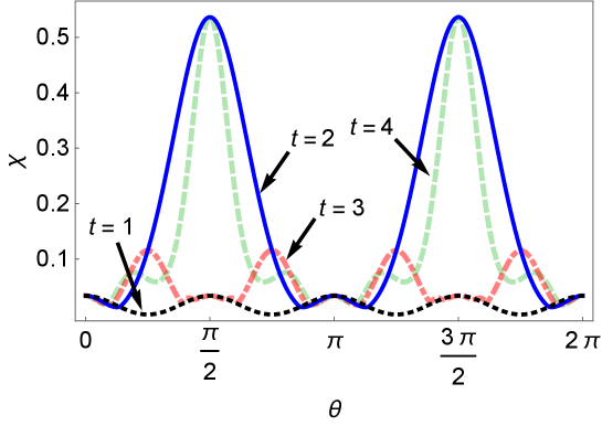
where the map is defined in Eq. (12). Figure (4) depicts the behavior of trace distance under this composite map, where RTN is operated both in Markovian and non-Markovian regimes. The non-monotonic behavior of trace distance in the Markovian regime of RTN channel is a consequence of the inherent non-Makovian nature of the reduced coin dynamics.
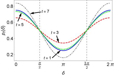
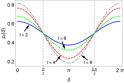
III.2 Purity and mixedness under QW channel
The purity of a state quantifies the degree of disorder or mixedness in it. The system-environment interaction is often accompanied with a loss of coherence in the state leading to mixedness. Thus, purity and mixedness are complementary quantities connected by the following relation Singh et al. (2015)
| (21) |
Here, is the mixedness and is the purity of the -dimensional state . Figure 5 (a)-(b) depict the purity of the output state of QW channel when the input state is . For both even and odd number steps, the system is found to be in pure state for . The same quantity is depicted in Fig. 5 (c)-(d), with respect to the coin parameter , for state parameter .
 |
 |
| (a) | (b) |
 |
 |
| (c) | (d) |
III.3 Holevo quantity for QW channel
When a state is subjected to a noise channel, its quantum features get affected, usually manifested in the form of decoherence and dissipation. The amount of information about the input state that can be retrieved from the output state is known as accessible information. The accessible information is upper bounded by the Holevo quantity Srikanth and Banerjee (2008) defined as
| (22) |
Here, is the set of input states with probability with probability , describing the ensemble . The map in our case, represents the reduced coin dynamics, and is defined in Eq. (12). Let us consider a case when the input state is described by the ensemble , with and . For different number of steps, the Holevo quantity, maximized over and , with , is depicted in Fig. (6). One infers that the Holevo quantity is suppressed for odd number of steps.
IV Conclusion
Recent studies have reported the constructive role of non-Markovian quantum channels over Markovian ones, in enhancing various quantum features of the system. We have characterized the reduced coin dynamics in DTQW as a non-Markovian quantum channel by analytically computing the Kraus operators for a -step walk. The non-Markovianity is inferred from the P-divisibility, reflected by non-monotonous behavior of the trace distance between two orthogonal states subjected to the channel. Subtleties arising due to concatenation of one step map for number of steps are highlighted. This could be envisaged to have impact on the study of memory processes on QW evolutions. The impact of noisy channel on the purity of a quantum state is studied with respect to the number of steps as well as the channel (coin) parameter. The amount of information about an input state which can be retrieved from the output, is bounded by Holevo quantity, and is shown to exhibit different behavior for even and odd number of steps. The QW channels, introduced here, add to the important class of non-Markovian channels which help in developing characterization methods for open quantum systems and strategies for various quantum information tasks. Feasibility of experimental implementation of DTQW in various quantum systems can lead way towards practical realization of non-Markovian quantum channels presented in this work.
Acknowledgment
JN would like to acknowledge the support from The Institute of Mathematical Sciences, Chennai to visit them during the completion of this work. CMC would like to acknowledge the support from DST, government of India under Ramanujan Fellowship grant no. SB/S2/RJN-192/2014.
Appendix
Calculation of :
From the definition
| (23) |
Note that . We propose
| (24) |
We will prove this by induction. The cases with and trivially hold. Let us assume the results holds for , so that
| (25) |
The upper limit of is restricted to , since , therefore, for we have , that is greater than the original limit of . Similarly, one can show
| (26) |
| Steps | Kraus operators |
|---|---|
| 1 | |
| 2 | |
| 3 |
References
- Breuer et al. (2002) H.-P. Breuer, F. Petruccione, et al., The theory of open quantum systems (Oxford University Press on Demand, 2002).
- Banerjee (2018) S. Banerjee, Open Quantum Systems: Dynamics of Nonclassical Evolution, Vol. 20 (Springer, 2018).
- Huelga et al. (2012) S. F. Huelga, A. Rivas, and M. B. Plenio, Phys. Rev. Lett. 108, 160402 (2012).
- Laine et al. (2014) E.-M. Laine, H.-P. Breuer, and J. Piilo, Scientific reports 4, 4620 (2014).
- Vasile et al. (2011) R. Vasile, S. Olivares, M. A. Paris, and S. Maniscalco, Phys. Rev. A 83, 042321 (2011).
- Chin et al. (2012) A. W. Chin, S. F. Huelga, and M. B. Plenio, Phys. Rev. Lett. 109, 233601 (2012).
- Thorwart et al. (2009) M. Thorwart, J. Eckel, J. Reina, P. Nalbach, and S. Weiss, Chemical Physics Letters 478, 234–237 (2009).
- Riazanov (1958) G. Riazanov, JETP 6, 1107 (1958).
- Feynman (1986) R. P. Feynman, Foundations of physics 16, 507 (1986).
- Parthasarathy (1988) K. Parthasarathy, Journal of applied probability , 151 (1988).
- Meyer and Shakeel (2016) D. A. Meyer and A. Shakeel, Phys. Rev. A 93, 012333 (2016).
- Wong and Meyer (2016) T. G. Wong and D. A. Meyer, Physical Review A 93 (2016), 10.1103/physreva.93.062313.
- Aharonov et al. (1993) Y. Aharonov, L. Davidovich, and N. Zagury, Phys. Rev. A 48, 1687 (1993).
- Shenvi et al. (2003) N. Shenvi, J. Kempe, and K. B. Whaley, Physical Review A 67, 052307 (2003).
- Krovi and Brun (2006) H. Krovi and T. A. Brun, Physical Review A 73, 032341 (2006).
- Srikanth et al. (2010) R. Srikanth, S. Banerjee, and C. Chandrashekar, Physical Review A 81, 062123 (2010).
- Chandrashekar et al. (2012) C. M. Chandrashekar, S. K. Goyal, and S. Banerjee, Journal of Quantum Information Science 02, 15–22 (2012).
- Rao et al. (2011) B. R. Rao, R. Srikanth, C. Chandrashekar, and S. Banerjee, Physical Review A 83, 064302 (2011).
- Chandrashekar et al. (2007) C. Chandrashekar, R. Srikanth, and S. Banerjee, Physical Review A 76, 022316 (2007).
- Banerjee et al. (2008) S. Banerjee, R. Srikanth, C. Chandrashekar, and P. Rungta, Physical Review A 78, 052316 (2008).
- Kumar et al. (2018) N. P. Kumar, S. Banerjee, and C. Chandrashekar, Scientific reports 8, 1 (2018).
- Chandrashekar et al. (2010) C. Chandrashekar, S. Banerjee, and R. Srikanth, Physical Review A 81, 062340 (2010).
- Chandrashekar and Banerjee (2011) C. Chandrashekar and S. Banerjee, Physics Letters A 375, 1553 (2011).
- Perets et al. (2008) H. B. Perets, Y. Lahini, F. Pozzi, M. Sorel, R. Morandotti, and Y. Silberberg, Phys. Rev. Lett. 100, 170506 (2008).
- Karski et al. (2009) M. Karski, L. Förster, J.-M. Choi, A. Steffen, W. Alt, D. Meschede, and A. Widera, Science 325, 174 (2009).
- Peruzzo et al. (2010) A. Peruzzo, M. Lobino, J. C. Matthews, N. Matsuda, A. Politi, K. Poulios, X.-Q. Zhou, Y. Lahini, N. Ismail, K. Wörhoff, et al., Science 329, 1500 (2010).
- Schreiber et al. (2010) A. Schreiber, K. N. Cassemiro, V. Potoček, A. Gábris, P. J. Mosley, E. Andersson, I. Jex, and C. Silberhorn, Phys. Rev. Lett. 104, 050502 (2010).
- Broome et al. (2010) M. A. Broome, A. Fedrizzi, B. P. Lanyon, I. Kassal, A. Aspuru-Guzik, and A. G. White, Phys. Rev. Lett. 104, 153602 (2010).
- Tamura et al. (2020) M. Tamura, T. Mukaiyama, and K. Toyoda, Physical Review Letters 124 (2020), 10.1103/physrevlett.124.200501.
- Kitagawa et al. (2012) T. Kitagawa, M. A. Broome, A. Fedrizzi, M. S. Rudner, E. Berg, I. Kassal, A. Aspuru-Guzik, E. Demler, and A. G. White, Nature communications 3, 1 (2012).
- Preiss et al. (2015) P. M. Preiss, R. Ma, M. E. Tai, A. Lukin, M. Rispoli, P. Zupancic, Y. Lahini, R. Islam, and M. Greiner, Science 347, 1229 (2015).
- Côté et al. (2006) R. Côté, A. Russell, E. E. Eyler, and P. L. Gould, New Journal of Physics 8, 156 (2006).
- Ryan et al. (2005) C. A. Ryan, M. Laforest, J. C. Boileau, and R. Laflamme, Phys. Rev. A 72, 062317 (2005).
- Qiang et al. (2016) X. Qiang, T. Loke, A. Montanaro, K. Aungskunsiri, X. Zhou, J. L. O’Brien, J. B. Wang, and J. C. F. Matthews, Nature Communications 7 (2016), 10.1038/ncomms11511.
- Alderete et al. (2020) C. H. Alderete, S. Singh, N. H. Nguyen, D. Zhu, R. Balu, C. Monroe, C. M. Chandrashekar, and N. M. Linke, (2020), arXiv:2002.02537 [quant-ph] .
- Chandrashekar (2006) C. Chandrashekar, Physical Review A 74, 032307 (2006).
- Dadras et al. (2018) S. Dadras, A. Gresch, C. Groiseau, S. Wimberger, and G. S. Summy, Phys. Rev. Lett. 121, 070402 (2018).
- Hoyer et al. (2010) S. Hoyer, M. Sarovar, and K. B. Whaley, New Journal of Physics 12, 065041 (2010).
- Mohseni et al. (2008) M. Mohseni, P. Rebentrost, S. Lloyd, and A. Aspuru-Guzik, The Journal of chemical physics 129, 11B603 (2008).
- Rebentrost et al. (2009) P. Rebentrost, M. Mohseni, I. Kassal, S. Lloyd, and A. Aspuru-Guzik, New Journal of Physics 11, 033003 (2009).
- Kumar et al. (2018) N. P. Kumar, S. Banerjee, R. Srikanth, V. Jagadish, and F. Petruccione, Open Systems and Information Dynamics 25, 1850014 (2018), arXiv:1711.03267 [quant-ph] .
- Hinarejos et al. (2014) M. Hinarejos, C. Di Franco, A. Romanelli, and A. Pérez, Physical Review A 89, 052330 (2014).
- Daffer et al. (2004) S. Daffer, K. Wódkiewicz, J. D. Cresser, and J. K. McIver, Phys. Rev. A 70, 010304 (2004).
- Van Kampen (1992) N. G. Van Kampen, Stochastic processes in physics and chemistry, Vol. 1 (Elsevier, 1992).
- Rivas et al. (2014) Á. Rivas, S. F. Huelga, and M. B. Plenio, Reports on Progress in Physics 77, 094001 (2014).
- Breuer et al. (2016) H.-P. Breuer, E.-M. Laine, J. Piilo, and B. Vacchini, Rev. Mod. Phys. 88, 021002 (2016).
- Shrikant et al. (2019) U. Shrikant, R. Srikanth, and S. Banerjee, arXiv:1911.04162 (2019).
- Chandrashekar (2010) C. Chandrashekar, arXiv:1001.5326 (2010).
- Wyss (2017) W. Wyss, arXiv:1707.03861 (2017).
- Singh et al. (2020) S. Singh, C. H. Alderete, R. Balu, C. Monroe, N. M. Linke, and C. Chandrashekar, arXiv:2001.11197 (2020).
- Singh et al. (2015) U. Singh, M. N. Bera, H. S. Dhar, and A. K. Pati, Physical Review A 91, 052115 (2015).
- Srikanth and Banerjee (2008) R. Srikanth and S. Banerjee, Phys. Rev. A 77, 012318 (2008).