Non-simple systoles on random hyperbolic surfaces for large genus
Abstract.
In this paper, we investigate the asymptotic behavior of the non-simple systole, which is the length of a shortest non-simple closed geodesic, on a random closed hyperbolic surface on the moduli space of Riemann surfaces of genus endowed with the Weil-Petersson measure. We show that as the genus goes to infinity, the non-simple systole of a generic hyperbolic surface in behaves exactly like .
1. Introduction
The study of closed geodesics on hyperbolic surfaces has deep connection to their spectral theory, dynamics and hyperbolic geometry. Let be a closed hyperbolic surface of genus . The systole of , the length of a shortest closed geodesic on , is always realized by a simple closed geodesic, i.e. a closed geodesic without self-intersections. The non-simple systole of is defined as
where is the length of in . It is known that is always realized as a figure-eight closed geodesic in (see e.g. [Bus10, Theorem 4.2.4]). In this work, we view the non-simple systole as a random variable on moduli space of Riemann surfaces of genus endowed with the Weil-Petersson probability measure . This subject was initiated by Mirzakhani in [Mir10, Mir13], based on her celebrated thesis works [Mir07a, Mir07b]. Firstly it is known that for all , (see e.g. [Yam82, Bus10]) and (see e.g. [BS94, Tor23]). In this paper, we show that as goes to infinity, a generic hyperbolic surface in has non-simple systole behaving like . More precisely, let be any function satisfying
| (1) |
Theorem 1.
For any satisfying (1), the following limit holds:
Remark.
It was shown in [NWX23, Theorem 4] that for any ,
As a direct consequence of Theorem 1, as goes to infinity, the asymtotpic behavior of the expected value of over can also be determined.
Theorem 2.
The following limit holds:
Proof.
Take and set . Define
By Theorem 1 we know that
Then firstly it is clear that
For the other direction, since for some universal constant (see e.g. Lemma 9),
The proof is complete. ∎
Remark.
The geometry and spectra of random hyperbolic surfaces under this Weil-Petersson measure have been widely studied in recent years. For examples, one may see [GPY11] for Bers’ constant, [Mir13, WX22b] for diameter, [MP19] for systole, [Mir13, NWX23, PWX22] for separating systole, [Mir13, WX22b, LW21, AM23] for first eigenvalue, [GMST21] for eigenfunction, [Mon22] for Weyl law, [Rud22, RW23] for GOE, [WX22a] for prime geodesic theorem, [Nau23] for determinant of Laplacian. One may also see [LS20, MT21, Hid22, SW22, HW22, HHH22, HT22, DS23, Gon23, MS23] and the references therein for more related topics.
A relative easier part is to prove the lower bound, that is to show that
| (2) |
We know that is realized by a figure-eight closed geodesic that is always filling in a unique pair of pants. And the length of such a figure-eight closed geodesic can be determined by the lengths of the three boundary geodesics of the pair of pants (see e.g. formula (17)). For and , denote by the number of figure-eight closed geodesics of length in . We view it as a random variable on . Then using Mirzakhani’s integration formula and change of variables, a direct computation shows that its expected value satisfies that as ,
| (3) |
Here we say if . Thus, we have
as . This in particular implies (2).
The hard part of Theorem 1 is the upper bound, that is to show that
| (4) |
Set and for any we define the following particular set and quantity:
and
It is not hard to see that there exists some universal constant such that
| (5) | ||||
To prove (4), it suffices to show
| (6) |
Using Mirzakhani’s integration formula and known bounds on Weil-Petersson volumes, direct computations show that (see Proposition 20),
| (7) |
Next we consider . For any , denote by the unique pair of pants bounded by and let be its completion in . Split as follows:
Then it is clear that
| (8) | ||||
Since for a pair of pants in , there exist at most different s such that , it follows from (7) that
| (9) |
Using Mirzakhani’s integration formula and known bounds on Weil-Petersson volumes, direct computations can show that (see Proposition 21 and 34)
| (10) |
and
| (11) |
Combining (7) and (10) gives the following important cancellation:
| (12) |
The crucial part is to bound . For this part, our method is inspired by the ones in [MP19, WX22b, NWX23]. Denote by the compact subsurface in of geodesic boundary such that is filling in it. Then one can divide as follows:
Through using the method in [WX22b] and the counting result on filling multi-geodesics in [WX22b, WX22a], we can show that (see Proposition 23)
| (13) |
For and , through classifying all the accurate relative positions of in both and , applying the McShane-Mirzakhani identity in [Mir07a] as for counting closed geodesics (we warn here that both the general counting result and the counting result in [WX22b, WX22a] on closed geodesics are inefficient to deal with these two cases), and then using Mirzakhani’s integration formula and known bounds on Weil-Petersson volumes, we can show that (see Proposition 24 and 28)
| (14) |
and
| (15) |
Then combining all these equations (7)—(15), one may finish the proof of (6), thus get (4) which is the upper bound in Theorem 1.
Notations. For any two nonnegative functions and (may be of multi-variables), we say if there exists a uniform constant such that . And we also say if and .
Plan of the paper. Section 2 will provide a review of relevant and necessary background materials. In Section 3 we compute the expectation of the number of figure-eight closed geodesics of length over which will imply (2), i.e. the lower bound in Theorem 1. In Section 4 we prove (4), i.e. the upper bound in Theorem 1. In which we apply the counting result on closed geodesics in [WX22b], and also apply the McShane-Mirzakhani identity in [Mir07a] to count closed geodesics for and .
Acknowledgement We would like to thank all the participants in our seminar on Teichmüller theory for helpful discussions on this project. The third named author is partially supported by the NSFC grant No. .
2. Preliminaries
In this section, we set our notations and recall certain relevant necessary results used in this paper, including Weil-Petersson metric, Mirzakhani’s integration formula, bounds on Weil-Petersson volumes, figure-eight closed geodesics and three countings on closed geodesics.
2.1. Moduli space and Weil-Petersson metric
Denote by an oriented topological surface with genus of punctures or boundaries where . Let be the Teichmüller space of surfaces with genus of punctures, and be the mapping class group of fixing the order of punctures. The moduli space of Riemann surfaces is . Denote and for simplicity. Given , let be the Teichmüller space of bordered hyperbolic surfaces with geodesic boundaries of lengths , and be the weighted moduli space. In particular, and .
Given a pants decomposition of , the Fenchel-Nielsen coordinates on the Teichmüller space is given by the map . Here is the length of on and is the twist along (measured by length). The following magic formula is due to Wolpert [Wol82]:
Theorem 3 (Wolpert).
The Weil-Petersson symplectic form on is given by
The form is mapping class group invariant. So it induces the so-called Weil-Petersson volume form on given by
Denote by the total volume of under the Weil-Petersson metric which is finite. Following [Mir13], we view a function as a random variable on with respect to the probability measure on , and we also denote by the expected value of over . Namely,
where is a Borel subset, is its characteristic function, and is short for .
2.2. Mirzakhani’s integration formula
In this subsection, we recall Mirzakhani’s integration formula in [Mir07a].
Let be a non-trivial and non-peripheral closed curve on topological surface and . Denote to be the hyperbolic length of the unique closed geodesic in the homotopy class of on . Let be an ordered k-tuple where the ’s are distinct disjoint homotopy classes of nontrivial, non-peripheral, unoriented simple closed curves on . Let be the orbit containing under the -action:
Given a function , one may define a function on :
Note that although can be only defined on , after taking sum , the function is well-defined on the moduli space .
For any , we set to be the moduli space of the hyperbolic surfaces (possibly disconnected) homeomorphic to with for every , where and are the two boundary components of given by cutting along . Assume . Consider the Weil-Petersson volume
where is the list of those coordinates of such that is a boundary component of . The following integration formula is due to Mirzakhani. One may see [Mir07a, Theorem 7.1], [Mir13, Theorem 2.2], [MP19, Theorem 2.2], [Wri20, Theorem 4.1] for different versions.
Theorem 4 (Mirzakhani’s integration formula).
For any , the integral of over with respect to the Weil-Petersson metric is given by
where the constant only depends on .
Remark.
One may see [Wri20, Theorem 4.1] for the detailed explanation and expression for the constant . We will give the exact value of only when required in this paper.
2.3. Weil-Petersson volumes
Denote to be the Weil-Petersson volume of and . In this subsection we only list the bounds for that we will need in this paper.
Theorem 5 ([Mir07a, Theorem 1.1]).
The initial volume . The volume is a polynomial in with degree . Namely we have
where lies in . Here is a multi-index and , .
Theorem 6.
Part (2) above can also be derived by [MZ15] of Mirzakhani-Zograf in which the precise asymptotic behavior of is provided for given .
Set . We also use the following quantity to approximate :
| (16) |
The estimation about sum of products of Weil-Petersson volumes can be found in e.g. [Mir13, MP19, GMST21, NWX23]. Here we use the following version:
Theorem 7 ([NWX23, Lemma 24]).
Assume , , . Then there exists two universal constants such that
where the sum is taken over all such that for all , and .
The following asymptotic behavior of was firstly studied in [MP19, Proposition 3.1]. We use the following version in [NWX23]. One may also see more sharp ones in [AM22].
Theorem 8 ([NWX23, Lemma 20]).
There exists a constant independent of and ’s such that
2.4. Figure-eight closed geodesics
Let be a hyperbolic surface. We say a closed geodesic in is a figure-eight closed geodesic if it has exactly one self-intersection point. Given a figure-eight closed geodesic , it is filling in a pair of pants with three geodesic boundary of lengths as shown in Figure 1. The length of the figure-eight closed geodesic is given by (see e.g. [Bus10, Equation (4.2.3)]):
| (17) |
It is clear that .
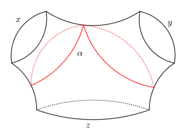
Remark.
In a pair of pants , there are exactly three different figure-eight closed geodesics of lengths , and . Here is the length of the figure-eight closed geodesic winding around and as shown in Figure 1.
It is known (see e.g. [Tor23, Lemma 5.2] or [Bus10, Section 5.2]) that the length of the shortest figure-eight closed geodesic in any is bounded.
Lemma 9.
There exists a universal constant independent of such that for any , the shortest figure-eight closed geodesic in has length .
Outline of the proof of Lemma 9.
Remark.
Recall that the non-simple systole of is defined as
We focus on figure-eight closed geodesics because the non-simple systole of a hyperbolic surface is always achieved by a figure-eight closed geodesic (see e.g. [Bus10, Theorem 4.2.4]). That is,
In particular, as introduced above we have
2.5. Three countings on closed geodesics
In this subsection, we mainly introduce three results about counting closed geodesics in hyperbolic surfaces. In this paper, we only consider primitive closed geodesics without orientations.
2.5.1. On closed hyperbolic surfaces
First, by the Collar Lemma (see e.g. [Bus10, Theorem 4.1.6]), we have that a closed hyperbolic surface of genus has most pairwisely disjoint simple closed geodesics of length . It is also known from [Bus10, Theorem 6.6.4] that for all and , there are at most closed geodesics in of length which are not iterates of closed geodesics of length . As a consequence, we have
Theorem 10.
For any and , there are at most primitive closed geodesics in of length .
2.5.2. On compact hyperbolic surfaces with geodesic boundaries
For compact hyperbolic surfaces with geodesic boundaries, the following result for filling closed multi-geodesics is useful.
Definition.
Let be a hyperbolic surface with boundaries. Let be an ordered -tuple where ’s are non-peripheral closed geodesics in . We say is filling in if each component of the complement is homeomorphic to either a disk or a cylinder which is homotopic to a boundary component of .
In particular, a filling -tuple is a filling closed geodesic in .
Define the length of a -tuple to be the total length of ’s, that is,
Define the counting function for to be
Theorem 11 ([WX22b, Theorem 4] or [WX22a, Theorem 18]).
For any , and , there exists a constant only depending on and such that for all and any compact hyperbolic surface of genus with boundary simple closed geodesics, the following holds:
Where is the total length of the boundary closed geodesics of .
2.5.3. On and
For the cases of and , we will apply the McShane-Mirzakhani identity to give more refined counting results on certain specific types of simple closed geodesics. The McShane-Mirzakhani identity states as:
Theorem 12 ([Mir07a, Theorem 1.3]).
For with geodesic boundaries of length respectively, we have
where the first sum is over all unordered pairs of simple closed geodesics bounding a pair of pants with , and the second sum is over all simple closed geodesics bounding a pair of pants with and . Here and are given by
and
The functions and have the following elementary properties:
Lemma 13 ([NWX23, Lemma 27]).
Assume that , then the following properties hold:
-
(1)
and .
-
(2)
is decreasing with respect to and increasing with respect to . is decreasing with respect to and and increasing with respect to .
-
(3)
We have
and
Theorem 14.
-
On a surface , the number of simple closed geodesics of length which bound a pair of pants with the two boundaries of lengths and has the upper bound
(18) -
On a surface , the number of simple closed geodesics of length which bound a pair of pants with the two boundaries of lengths and has the upper bound
(19) -
On a surface , the number of unordered pairs of simple closed geodesics of total length which bound a pair of pants with the boundary of length has the upper bound
(20)
Proof.
3. Lower bound
In this section we compute the expectation of the number of figure-eight closed geodesics of length over , and hence gives the lower bound of the length of non-simple systole for random hyperbolic surfaces.
Let and denote
and
to be the number of figure-eight closed geodesics in with length . Then the non-simple systole of has length if and only if .
The main result of this section is as follows.
Proposition 15.
For any and ,
where the implied constant is independent of and .
Let’s firstly assume Proposition 15 and prove the following direct consequence which is the lower bound in Theorem 1.
Theorem 16.
For any function satisfying
then we have
Proof.
Taking in Proposition 15, it is clear that
Then it follows by Markov’s inequality that
This also means that
Then the conclusion follows because for any , is equal to the length of a shortest figure-eight closed geodesic in . ∎
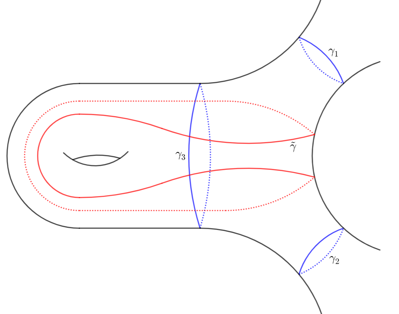
For a figure-eight closed geodesic , it is always filling in a unique pair of pants as shown in Figure 1. If two of the boundary geodesics in are the same simple closed geodesics in , then the completion of is a hyperbolic torus with one geodesic boundary; otherwise is still a pair of pants. So the complement may have one or two or three components (see Figure 2 for an illustation when ). We classify all figure-eight closed geodesics by the topology of . Denote
and
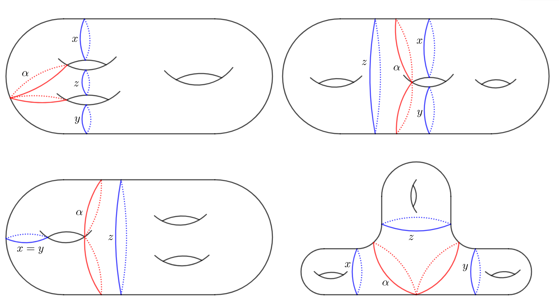
Upper right: has two components.
Lower left: is connected.
Lower right: has three components.
Then
where the first sum is taken over all with and ; the second sum is taken over all with and .
We now compute , and sum of all possible and in the following Lemmas.
Lemma 17.
For any and ,
where the implied constant is independent of and .
Proof.
Instead of a figure-eight closed geodesic, we consider the unique pair of pants (with three boundary lengths equal to ) in which a figure-eight closed geodesic is filling. In each pair of pants, there are exactly three figure-eight closed geodesics. And in the pair of pants , the number of figure-eight closed geodesics of length is equal to where is the length function given in (17). So the counting of figure-eight closed geodesics can be replaced by the counting of pairs of pants ’s satisfying . And by Mirzakhani’s integration formula Theorem 4 (here for the pair ), we have
| (22) | |||
where in the last equation we apply that and the product is symmetric with respect to . By Part (2) of Theorem 6 we have
| (23) |
This together with Theorem 8 imply that
| (24) |
Applying (24) into the last line of (22), by the fact that , the remainder term can be bounded as
And the main term is
| (26) |
We change the variables into with . By (17),
So
| (27) | |||
where the integration region Cond is
We consider the integral for and in order. First taking an integral for , we get
Then taking an integral for , we get
Finally taking an integral for , it is clear that , so we get
| (28) | |||
So combining (22), (3), (27) and (28), we obtain
as desired. ∎
Remark.
Similar computations were taken in [AM23].
Lemma 18.
For any and we have
where the first sum is taken over all with and ; the second sum is taken over all with and . The implied constants are independent of and .
Proof.
In a pair of pants , there are exactly three figure-eight closed geodesics. And from (17) we know that the condition that a figure-eight closed geodesic in has length can imply that and all . So
Then applying Mirzakhani’s integration formula Theorem 4 and Theorem 8,
and
| (30) | |||
and similarly
| (31) |
Then applying Theorem 6 and Theorem 7 for we have
| (32) |
| (33) |
| (34) |
4. Upper bound
In this section, we will prove the upper bound of the length of non-simple systole for random hyperbolic surfaces. That is, we show
Theorem 19.
For any function satisfying
then we have
In order to prove Theorem 19, it suffices to show that
| (35) |
where
Instead of working on , we consider defined as follows.
Definition.
For any and , denote by
and
It follows by Equation (17) that each bounds a pair of pants that contains a figure-eight closed geodesic of length for some uniform constant : acutally the desired figure-eight closed geodesic is the one winding around and . Then we have
| (36) | ||||
For any , we view as a nonnegative integer-valued random variable on . Then by the standard Cauchy-Schwarz inequality we know that
implying
| (37) | ||||
For any , denote by the pair of pants bounded by the three closed geodesics in . Set
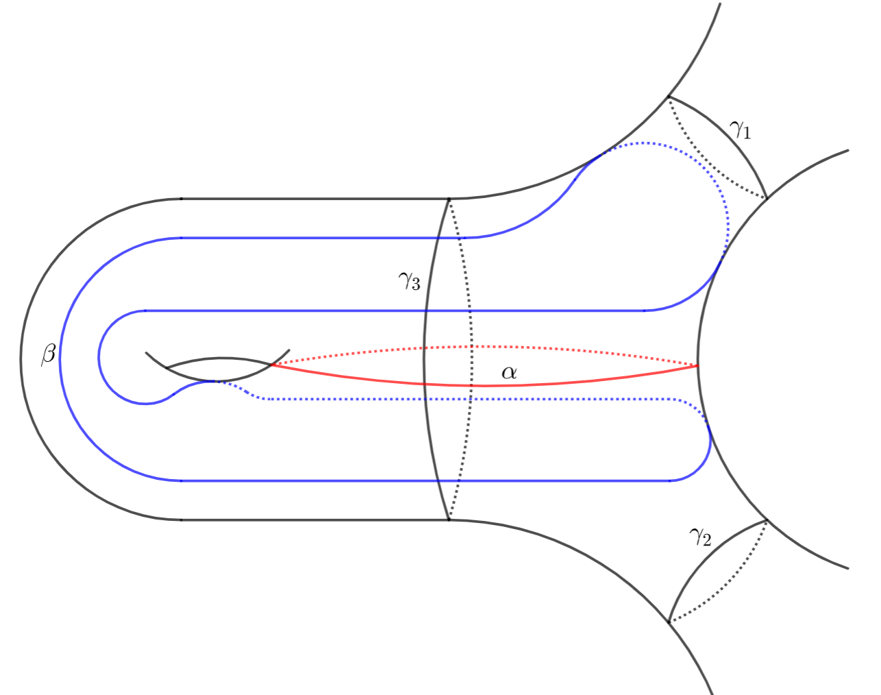
Assume and , as shown in Figure 3:
-
(1)
In the first picture, . Then we have and . Hence ;
-
(2)
In the second picture, . Hence and ;
-
(3)
In the third picture, . Hence ;
-
(4)
In the forth picture, and . Hence
Denote by
It is clear that
| (38) | ||||
Since for any pair of pants in , there exist at most different s such that , it follows that
| (39) |
Now we split the proof of Theorem 19 into the following several subsections. The estimate for is the hard part. And the estimates for and are relative easier.
4.1. Estimations of
Proposition 20.
Assume and , then
where the implied constant is independent of and .
Proof.
For any , let be a domain defined by
Assume is the characteristic function of , i.e.
Assume is a pair of ordered simple closed curves in such that
Apply Mirzakhani’s integration formula Theorem 4 to the ordered simple closed multi-curve and function , we have
| (41) | ||||
Recall that Equation (23) says that
| (42) |
By Theorem 8, for any , as , we have
| (43) |
where the implied constant is independent of and . So we have
| (44) | ||||
where the implied constant is independent of and . From direct calculations we have
| (45) |
and
| (48) | ||||
where the implied constants are independent of . From (45) and (48) we have
| (49) | ||||
| (52) | ||||
From (44), (49) and the assumption that , we obtain
as desired. ∎
4.2. Estimations of
For , we will show that
where and . More precisely,
Proposition 21.
Assume and , then
| (53) |
where the implied constant is independent of and .
Proof.
Assume and , . From the definition of , it is not hard to check that
Define a function as follows:
where is defined in the proof of Proposition 20. Assume is an ordered simple closed multi-curve in such that
where the boundary of consists of and the boundary of consists of . By Part of Theorem 6 we have
| (54) |
By Theorem 8 we have
| (55) |
where the implied constant is independent of and . Applying Mirzakhani’s integration formula Theorem 4 to ordered simple closed multi-curve and function , together with (49), (54) and (55), we have
| (56) | |||
where the implied constant is independent of and . ∎
4.3. Estimations of
For , is not the union of disjoint simple closed geodesics but with intersections. This is the hard case. We will need the following construction as in [MP19, WX22b, NWX23] to deform .
Construction.
Fix a closed hyperbolic surface and let be two distinct connected, precompact subsurfaces of with geodesic boundaries, such that and neither of them contains the other. Then the union is a subsurface whose boundary consists of only piecewise geodesics. We can construct from it a new subsurface, with geodesic boundary, by deforming each of its boundary components as follows:
-
(1)
if is homotopically nontrivial, we deform by shrinking to the unique simple closed geodesic homotopic to it;
-
(2)
if is homotopically trivial, we fill into the disc bounded by .
Denote by the subsurface with geodesic boundary constructed from and as above. For any , denote by the subsurface of constructed from and .
By the construction, it is clear that
| (57) |
and by isoperimetric inequality(see e.g. [Bus10, Section 8.1] or [WX22c]) we have
| (58) |
Recall that by the definition of , we know that for any ,
Thus we may divide into following pairwisely disjoint three parts:
| (59) |
where
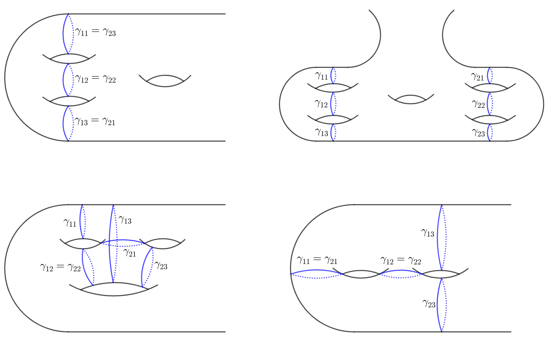
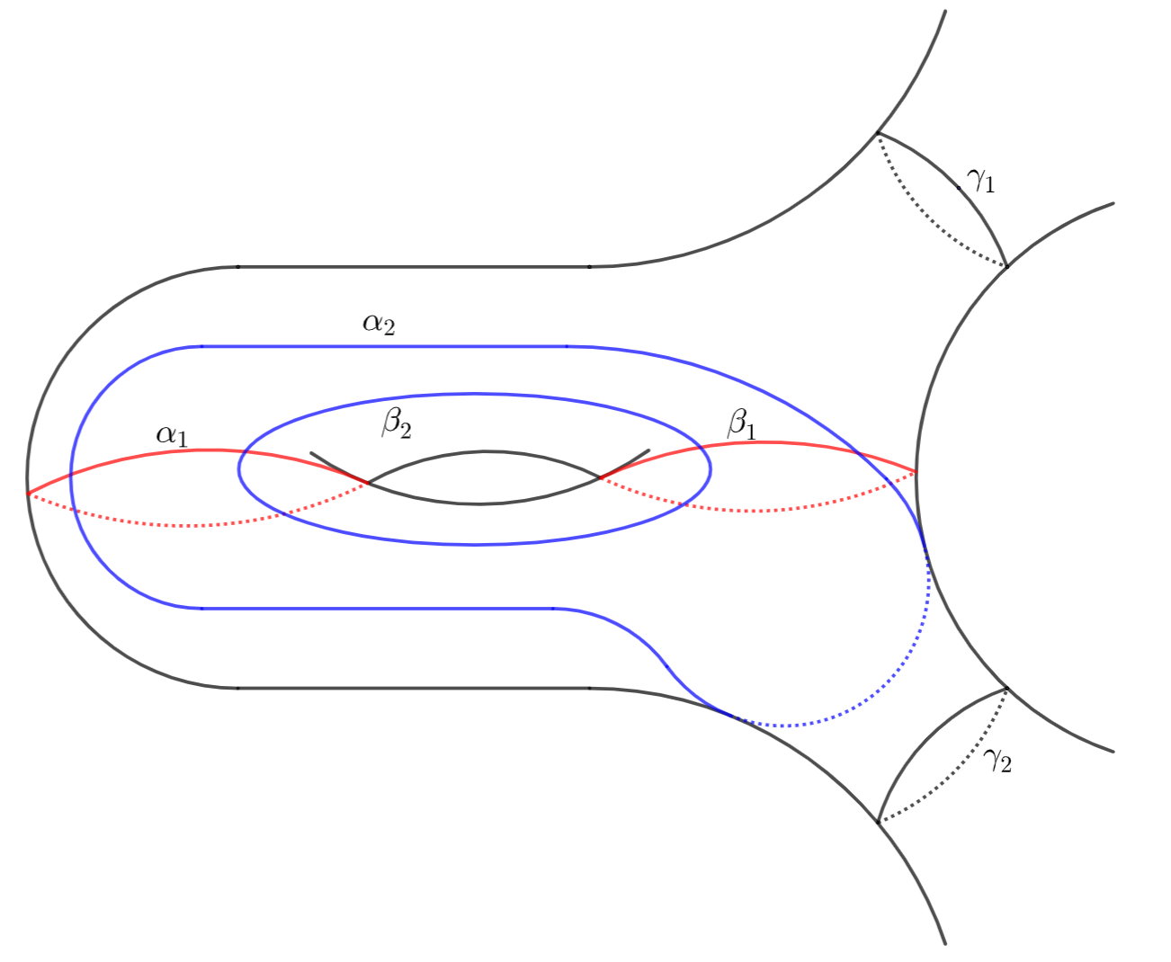
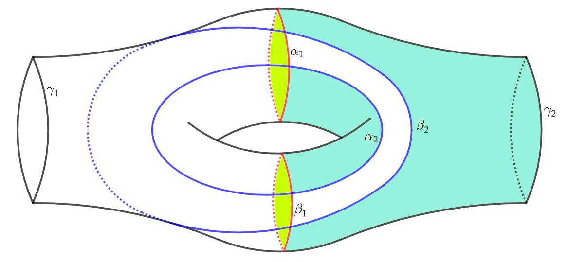
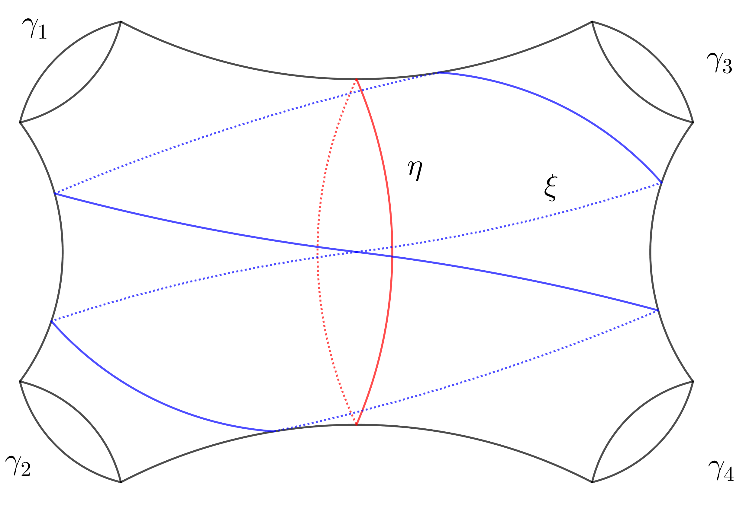
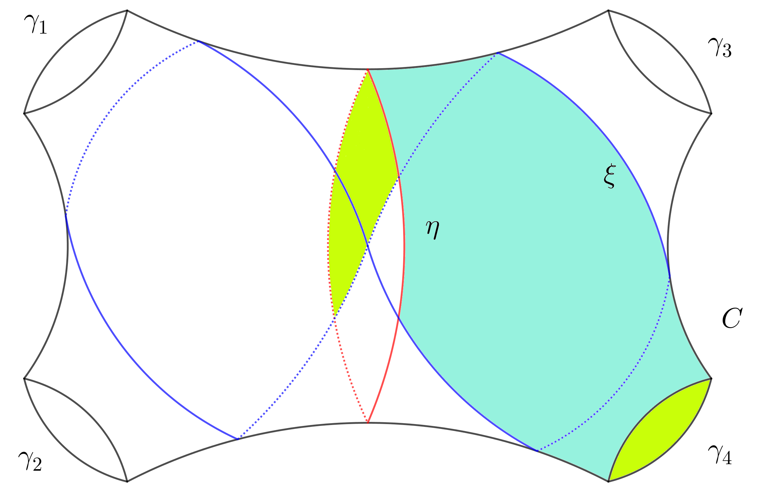
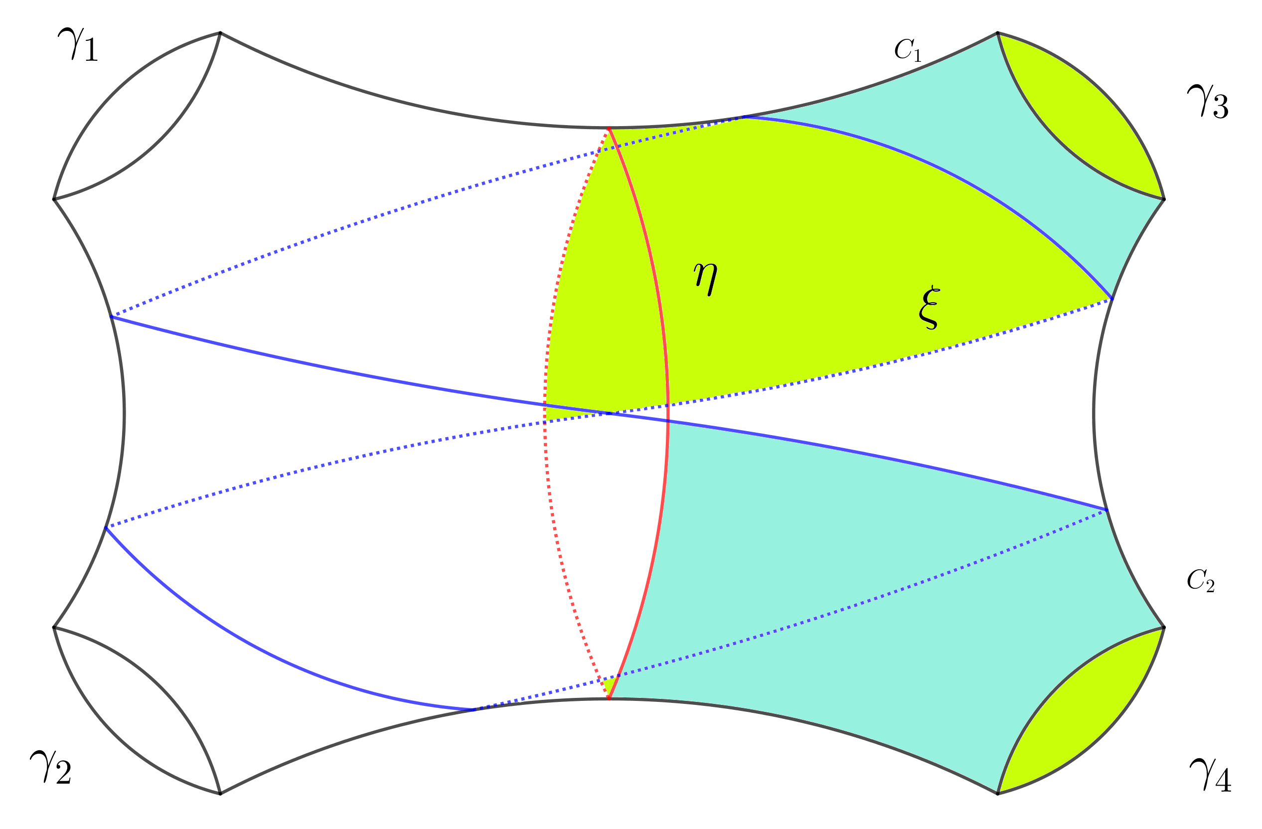
Assume and . As in Figure 4:
-
(1)
in the first picture, the simple closed geodesic coincides with . We have of geodesic boundaries and . Hence ;
-
(2)
in the second picture, we have of geodesic boundaries and . Hence ;
-
(3)
in the third picture, we have of geodesic boundaries where and appear twice in the boundary of . Hence .
For and , define
Lemma 22.
For any , there exists a triple and a universal constant such that
-
(1)
;
-
(2)
is a figure-eight closed geodesic contained in for ;
-
(3)
is a filling 2-tuple in and .
Proof.
Part (2) is clear.
For Part (3), we first assume . For , let be the figure-eight closed geodesic contained in winding around and . Then from (17) we have
| (60) |
From the assumption that , we have
| (61) |
From (60) and (61), one may check that there exists a universal constant such that . Now we show that is a filling 2-tuple in . Suppose not, then there exists a simple closed geodesic in such that Since fills , it follows that . Then by the construction of we have , which is a contradiction.
The proof is complete. ∎
Similar to [WX22b], we set the following assumption.
Assumption . Let satisfying
-
(1)
is homeomorphic to to for some and with ;
-
(2)
the boundary is a simple closed multi-geodesics in consisting of simple clsoed geodesics which has pairs of simple closed geodesics for some such that each pair corresponds to a single simple closed geodesic in ;
-
(3)
the interior of its complement consists of components for some where .
Our aim is to bound , from (59) it suffices to bound the three terms and separately.
4.3.1. Bounds for
We first bound through using the method in [WX22b].
Proposition 23.
Assume and , then for any fixed small ,
Proof.
For , by Lemma 22, there exists a filling 2-tuple in with total length , and is a filling figure-eight closed geodesic in a unique pair of pants for both respectively. Consider the alternatives of three geodesics in elements in , there are at most pairs corresponding to the same triples . It follows that
where is defined in Subsection 2.5.2. Therefore we have
| (62) |
Now we divide the summation above into following two parts: the first part consists of all subsurfaces such that ; the second part consists of all subsurfaces such that .
For the first part, assume satisfies Assumption with an additional assumption that
| (63) |
From [WX22b, Proposition 34] and Theorem 11, we have that for any fixed ,
| (64) | ||||
Since there are at most finite pairs satisfying the assumption (63), take summation over all possible subsurfaces for inequality (64), we have
| (65) |
4.3.2. Bounds for
One may be aware of that the method in Proposition 23 cannot afford desired estimations for and . Our aim for is as follows.
Proposition 24.
For and large ,
The estimations for pairs with in Lemma 22 are not good enough. We need to accurately classify the relative position of in . We begin with the following bounds.
Lemma 25.
For and ,
| (68) | ||||
where are taken over all triples of simple closed geodesics on satisfying that cuts off a subsurface in and separates into
Proof.
For any such that either or contains , WLOG, one may assume that and contains . Denote the rest simple closed geodesic in by . Consider the map
where the union cuts off in and separates into with length
| (69) |
Now we count all ’s satisfying and . Since and , it is clear that must contain at least one of and .
Case-1: contains (see Figure 5 for an illustation). For this case, the remaining simple closed geodesic in is of length and bounds a in along with as in Figure 5. Then it follows by (19) that the number of such ’s is at most
Case-2: contains only one of (see Figure 6 for an illustation). WLOG, one may assume that contains only . Then the rest two simple closed geodesics in , along with , will bound a in of total length as in Figure 6. Then it follows by (20) that the number of such pairs of ’s is at most
Combine these two cases, we have
Then the conclusion follows by taking a summation over all possible ’s satisfying (69). This completes the proof. ∎
Remark.
The coefficient in the proof of Lemma 25 comes from the symmetry of the three boundary components of a pair of pants, the symmetry of and , and is not essential. What we need is a universal positive constant.
Lemma 26.
For and ,
| (70) | ||||
where are taken over all quadruples satisfying that cuts off a subsurface in and separates into with belonging to the boundaries of the two different ’s.
Proof.
For any belonging to the set in the left side of (70), WLOG, one may assume that , , only contains and only contains . The rest two simple closed geodesics in will separate into , i.e. two copies of . Consider the map
where the union cuts off in , and separates into such that belong to the boundaries of two different ’s (see Figure 7 for an illustation). Moreover, their lengths satisfy
| (71) |
Then we count all ’s such that with and . Such a is uniquely determined by the rest two simple closed geodesics in whose union separates into with in two different ’s, of length as shown in Figure 7.
Lemma 27.
For and ,
| (72) | ||||
where are taken over all quadruples satisfying that cuts off a subsurface in and separates into with belonging to the boundaries of two different ’s.
Proof.
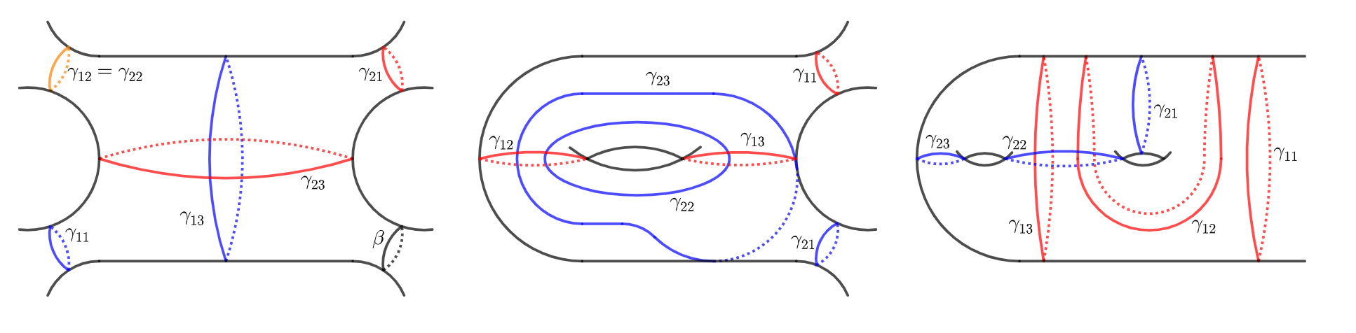
For any belonging to the set in the left side of (72), WLOG, one may assume that , , both and contain and do not contain . Assume that contains and contains . In this situation, we warn here that may exceed . Since fills , there is a connected component of such that is topologically a cylinder and is a connected component of . The other connected component of , denoted by , is a closed piecewisely smooth geodesic loop, freely homotopical to . Each geodesic arcs in are different parts of arcs in as shown in Figure 8. Firstly it is clear that
| (73) |
Since , we have
| (74) |
It follows from (73) and (74) that
| (75) |
Consider the map
for belonging to the set in the left side of (72). Here cuts off in and separates into such that belong to boundaries of two different ’s. Moreover, their lengths satisfy
| (76) |
Then we count all possible ’s such that , and . Since , it follows by (20) that there are at most
such pairs of ’s. This implies that
Sum it over all possible ’s satisfying (76), we complete the proof. ∎
Now we are ready to Proposition 24.
Proof of Proposition 24.
Following Lemma 25, Lemma 26 and Lemma 27, for we have
| (77) | ||||
where cuts off in , separates into , and separates into with in boundaries of two different ’s.
For in , the completion subsurface can be of type either or with . By Mirzakhani’s integration formula, i.e. Theorem 4, Theorem 5, Theorem 8, and Theorem 13, we have that for ,
| (78) | ||||
where are taken over all possible and .
Similarly, by Mirzakhani’s integration formula, i.e. Theorem 4, Theorem 5, Theorem 8, and Theorem 13, we have that for ,
| (79) | ||||
where are taken over all possible and .
4.3.3. Bounds for
Our aim for is as follows. The proof is similar as the one in bounding .
Proposition 28.
For and large ,
When , two boundary geodesics of may be the same closed geodesic in , in this case, the completion ; otherwise . Moreover, each of and has exactly two closed geodesics contained in the boundary of . Now we define
and set
For in view as the result surface of cutting along a non-separating simple closed geodesic. Then the number of elements in has same estimations as in Lemma 25, Lemma 26 and Lemma 27. Therefore, the proof of Proposition 24 yields that
Proposition 29.
For and large ,
Now we consider . Again we need to accurately classify elements in it according to the relative position of in The first one is as follows.
Lemma 30.
For and , we have
| (82) | ||||
where are taken over all quintuples satisfying that cuts off a subsurface in and bounds a in along with .
Proof.
For any belonging to the set in the left side of (82), WLOG, one may assume that , and contains . Then it follows that contains . Assume the rest simple closed geodesic in is and the rest simple closed geodesic in is as shown in Figure 9. Consider the map
where cuts off a subsurface in and bounds a along with in . Moreover their lengths satisfy
| (83) |
and
| (84) |
Then we count all possible ’s such that , and . We only need to count all possible ’s of length , each of which bounds a in along with It follows by (18) that there are at most
such ’s. So we have that
Then the proof is completed by taking a summation over all possible quintuples ’s satisfying (83) and (84). ∎
Lemma 31.
For and , we have
| (85) | ||||
where are taken over all quintuples satisfying that cuts off a subsurface in and bounds a in along with .
Proof.
For any belonging to the set in the left side of (85), WLOG, one may assume that , contains and contains . Assume that the rest simple closed geodesic in is and the rest simple closed geodesic in is as shown in Figure 10.
In this case, may exceed . However, since fills , there is a connected component of such that is topologically a cylinder and is a connected component of . The other connected component of , is the union of some geodesic arcs on It follows that
| (86) |
Since then we have
| (87) |
It follows from (86) and (87) that
| (88) |
Consider the map
where cuts off a in and cuts off a in along with . Moreover their lengths satisfy
| (89) | ||||
Then we count all possible ’s such that and . We only need to count all possible ’s of length , which bounds a in along with It follows by (18) that there are at most
such ’s. So we have that
Then the proof is completed by taking a summation over all possible quintuples ’s satisfying (89). ∎
Lemma 32.
For and , we have
| (90) | ||||
where are taken over all quintuples satisfying that cuts off a subsurface in and bounds a in along with .
Proof.
For any belonging to the set in the left side of (90), WLOG, one may assume that , and both contain . Assume the rest simple closed geodesic in is and the rest simple closed geodesic in is . Then both and will bound a in along with as shown in Figure 11.
In this case, both and may exceed . Since fills , there are two connected components of such that both are topologically cylinders, is a connected component of and is a connected component of . The other connected components of and , are the union of different geodesic arcs on It is clear that
| (91) |
Since we have
| (92) |
Then It follows from (91) and (92) that
Consider the map
where cuts off a in and cuts off a in along with . Moreover their lengths satisfy
| (93) | ||||
Then we count all possible ’s such that . We only need to count all possible ’s of length , each of which bounds a in along with It follows by (18) that there are at most
such ’s. So we have
Sum it over all possible quintuples ’s satisfying (93), we complete the proof. ∎
For , the complement subsurface can be one of five types: (1) ; (2) with and ; (3) with and ; (4) with and ; (5) with and . Set
to be the Weil-Petersson volume of the moduli space of Riemann surfaces each of which is homeomorphic to with geodesic boundaries of lengths . Define
and
Now we are ready to bound .
Proposition 33.
For and large ,
Proof.
Following Lemma 30, Lemma 31 and Lemma 32, we have that for ,
| (95) | ||||
where are taken over all quintuples satisfying that cuts off a subsurface in and bounds a in along with . Set
Then by Mirzakhani’s integration formula Theorem 4, Theorem 5, Theorem 8 and Theorem 13, we have that for ,
| (96) | ||||
Set
and
Similarly, by Mirzakhani’s integration formula Theorem 4, Theorem 5, Theorem 8 and Theorem 13, we have
| (97) | ||||
and
Now we are ready to prove Proposition 28.
4.4. Estimations of
For this part, we always assume that . We will show that as ,
More precisely,
Proposition 34.
For , we have
Proof.
For , the two pairs of pants and will share one or two simple closed geodesic boundary components. For the first case, assume that and . For the second case, assume that and . By the definition of , any two simple closed geodesics in have total length . So does . We have
| (100) | ||||
Here are taken over all quintuples satisfying that cuts off a subsurface in and bounds a in along with ; and while are taken over all quadruples satisfying that cuts off a subsurface in and separates into with belonging to the boundaries of the two different ’s. Set
By Mirzakhani’s integration formula Theorem 4, Theorem 5, Theorem 8 and (94), for we have
| (101) | ||||
Where in the last inequality we apply
For the remaining term, it follows by Mirzakhani’s integration formula Theorem 4, Theorem 5, Theorem 8 and (81) that for ,
| (102) | ||||
Combine (100), (101) and (102), we have
This completes the proof. ∎
4.5. Finish of the proof
Now we are ready to complete the proof of Theorem 19.
Proof of Theorem 19.
Take with . By (37) and (38) we have
| (103) | ||||
By Proposition 20 and Proposition 21 we have
| (104) |
By (39) and Proposition 20, for we have
| (105) |
By Proposition 20, Proposition 23, Proposition 24 and Proposition 28, fix , we have
| (106) |
By Proposition 20 and Proposition 34 we have
| (107) |
Therefore if , by (103), (104), (105), (106) and (107), we have
It follows that (35) holds by (36). This finishes the proof of Theorem 19. ∎
References
- [AM22] Nalini Anantharaman and Laura Monk, A high-genus asymptotic expansion of Weil-Petersson volume polynomials, J. Math. Phys. 63 (2022), no. 4, Paper No. 043502, 26.
- [AM23] Nalini Anantharaman and Laura Monk, Friedman-Ramanujan functions in random hyperbolic geometry and application to spectral gaps, arXiv e-prints (2023), arXiv:2304.02678.
- [BS94] P. Buser and P. Sarnak, On the period matrix of a Riemann surface of large genus, Invent. Math. 117 (1994), no. 1, 27–56, With an appendix by J. H. Conway and N. J. A. Sloane.
- [Bus10] Peter Buser, Geometry and spectra of compact Riemann surfaces, Modern Birkhäuser Classics, Birkhäuser Boston, Ltd., Boston, MA, 2010, Reprint of the 1992 edition.
- [DS23] Benjamin Dozier and Jenya Sapir, Counting geodesics on expander surfaces, arXiv:2304.07938.
- [GMST21] Clifford Gilmore, Etienne Le Masson, Tuomas Sahlsten, and Joe Thomas, Short geodesic loops and norms of eigenfunctions on large genus random surfaces, Geom. Funct. Anal. 31 (2021), 62–110.
- [Gon23] Yulin Gong, Spectral Distribution of Twisted Laplacian on Typical Hyperbolic Surfaces of High Genus, arXiv e-prints (2023), arXiv:2306.16121.
- [GPY11] Larry Guth, Hugo Parlier, and Robert Young, Pants decompositions of random surfaces, Geom. Funct. Anal. 21 (2011), no. 5, 1069–1090.
- [HHH22] Xiaolong Hans Han, Yuxin He, and Han Hong, Large Steklov eigenvalue on hyperbolic surfaces, arXiv e-prints (2022), arXiv:2210.06752.
- [Hid22] Will Hide, Spectral Gap for Weil–Petersson Random Surfaces with Cusps, International Mathematics Research Notices (2022), rnac293.
- [HT22] Will Hide and Joe Thomas, Short geodesics and small eigenvalues on random hyperbolic punctured spheres, arXiv e-prints (2022), arXiv:2209.15568.
- [HW22] Yuxin He and Yunhui Wu, On second eigenvalues of closed hyperbolic surfaces for large genus, arXiv e-prints (2022), arXiv:2207.12919.
- [LS20] Etienne Le Masson and Tuomas Sahlsten, Quantum ergodicity for Eisenstein series on hyperbolic surfaces of large genus, Mathematische Annalen (2020), to appear.
- [LW21] Michael Lipnowski and Alex Wright, Towards optimal spectral gaps in large genus, Annals of Probability (2021), to appear.
- [Mir07a] Maryam Mirzakhani, Simple geodesics and Weil-Petersson volumes of moduli spaces of bordered Riemann surfaces, Invent. Math. 167 (2007), no. 1, 179–222.
- [Mir07b] by same author, Weil-Petersson volumes and intersection theory on the moduli space of curves, J. Amer. Math. Soc. 20 (2007), no. 1, 1–23.
- [Mir10] by same author, On Weil-Petersson volumes and geometry of random hyperbolic surfaces, Proceedings of the International Congress of Mathematicians. Volume II, Hindustan Book Agency, New Delhi, 2010, pp. 1126–1145.
- [Mir13] by same author, Growth of Weil-Petersson volumes and random hyperbolic surfaces of large genus, J. Differential Geom. 94 (2013), no. 2, 267–300.
- [Mon22] Laura Monk, Benjamini-Schramm convergence and spectra of random hyperbolic surfaces of high genus, Anal. PDE 15 (2022), no. 3, 727–752.
- [MP19] Maryam Mirzakhani and Bram Petri, Lengths of closed geodesics on random surfaces of large genus, Comment. Math. Helv. 94 (2019), no. 4, 869–889.
- [MS23] Laura Monk and Rares Stan, Spectral convergence of the Dirac operator on typical hyperbolic surfaces of high genus, arXiv e-prints (2023), arXiv:2307.01074.
- [MT21] Laura Monk and Joe Thomas, The Tangle-Free Hypothesis on Random Hyperbolic Surfaces, International Mathematics Research Notices (2021), to appear.
- [MZ15] Maryam Mirzakhani and Peter Zograf, Towards large genus asymptotics of intersection numbers on moduli spaces of curves, Geom. Funct. Anal. 25 (2015), no. 4, 1258–1289.
- [Nau23] Frédéric Naud, Determinants of Laplacians on random hyperbolic surfaces, arXiv e-prints (2023), arXiv:2301.09965.
- [NWX23] Xin Nie, Yunhui Wu, and Yuhao Xue, Large genus asymptotics for lengths of separating closed geodesics on random surfaces, J. Topol. 16 (2023), no. 1, 106–175.
- [PWX22] Hugo Parlier, Yunhui Wu, and Yuhao Xue, The simple separating systole for hyperbolic surfaces of large genus, J. Inst. Math. Jussieu 21 (2022), no. 6, 2205–2214.
- [Rud22] Zeév Rudnick, GOE statistics on the moduli space of surfaces of large genus, arXiv e-prints (2022), arXiv:2202.06379.
- [RW23] Zeév Rudnick and Igor Wigman, Almost sure GOE fluctuations of energy levels for hyperbolic surfaces of high genus, arXiv e-prints (2023), arXiv:2301.05964.
- [SW22] Yang Shen and Yunhui Wu, Arbitrarily small spectral gaps for random hyperbolic surfaces with many cusps, arXiv e-prints (2022), arXiv:2203.15681.
- [Tor23] Tina Torkaman, Intersection Number, Length, and Systole on Compact Hyperbolic Surfaces, arXiv e-prints (2023), arXiv:2306.09249.
- [Wol82] Scott Wolpert, The Fenchel-Nielsen deformation, Ann. of Math. (2) 115 (1982), no. 3, 501–528.
- [Wri20] Alex Wright, A tour through Mirzakhani’s work on moduli spaces of Riemann surfaces, Bull. Amer. Math. Soc. (N.S.) 57 (2020), no. 3, 359–408.
- [WX22a] Yunhui Wu and Yuhao Xue, Prime geodesic theorem and closed geodesics for large genus, arXiv e-prints (2022), arXiv:2209.10415.
- [WX22b] Yunhui Wu and Yuhao Xue, Random hyperbolic surfaces of large genus have first eigenvalues greater than , Geom. Funct. Anal. 32 (2022), no. 2, 340–410.
- [WX22c] by same author, Small eigenvalues of closed Riemann surfaces for large genus, Trans. Amer. Math. Soc. 375 (2022), no. 5, 3641–3663.
- [Yam82] Akira Yamada, On Marden’s universal constant of Fuchsian groups. II, J. Analyse Math. 41 (1982), 234–248.