Non-spherical multicluster approximation in light nuclei
Abstract
Multicluster models consider that the nucleons can be moving around different centers in the nuclei. These models have been widely used to describe light nuclei but always considering that the mean field is composed of isotropic harmonic oscillators with different centers. In this work, we propose an extension of these models by using anisotropic harmonic oscillators. The strenghts of these oscillators, the distance among the different centers and the disposition of the nucleons inside every cluster are free parameters which have been fixed using the variational criterion. We have used a hamiltonian with the kinetic energy terms and a phenomenological two-body potential like Volkov V2 potential. All the one-body and two-body matrix elements have been analytically calculated. Only a numerical integration on the Euler angles, it is needed to carry out the projection on the values of the total spin of the state and its third component. We have studied the ground state and the first excited states of 8Be, 12C and 10Be getting good results for the energies. The disposition of the nucleons in the different clusters have been also analyzed by using projection on the different cartesian planes getting much more information than when the radial one-body density is used.
1 Introduction.
In light nuclei, the differences of the bound energy among deuteron, triton and, mainly, the particle, are arguments that allow to consider that nucleons in the stationary states can be located around more than one point in the space forming clusters of nucleons, being the particle the main way of clustering. Microscopic multicluster models have widely developed this form of describing the structure of stationary states since Wheeler proposed the Resonating Group Model (RGM) up to describe the ground state of 8Be as a pair of separated particles moving around each other [1]. Four years after, Margenau [2] presented an alternative to RGM that avoided some of its antisymmetrization problems by describing the eigenstates using Slater determinants with single particle wave functions centered around several fixed points in space. This proposal is generalized by Griffin and Wheeler with the Generator Coordinate Method (GCM) that leaves free the positions of the centers of the clusters [3]. The previously cited works joined to the further systematization of GCM by Brink [4, 5] are the background of all the models that have utilized the idea of different clusters of nucleons within nuclei. The most general models eliminate the restriction that clusters are only formed by particles, and drive to a molecular vision of nuclei [6] and are known as -cluster or multicluster models.
Multicluster models in their different versions have been widely used to study different aspects of the dynamics of light and medium nuclei. Important results on the structure and spectroscopy of the stationary states of nuclei up to 40Ca have been achieved [7, 8, 9], moreover they are of great utility to describe nuclei rich in neutrons specially when Antisymmetric Molecular Dynamics (AMD) is used [10, 11, 12]. The structure of multicluster vectors have also allowed to obtain cuantitative results in the description of nuclear reactions that involve light and medium nuclei [13, 14, 15]. A complete presentation of the theoretical aspects of this kind of approximations and of the specific applications can be found in the work by Descouvemot and Dufour [16] or in the one by von Oertzen, Freer and Kanada-En’yo [17].
Multicluster models can be considered as an independent particle approximation in which nucleons move in a mean potential with more than one minimum in contrast with the usual model where nucleons move in a local or non-local one-particle potential with a well defined minimum and with spherical symmetry. This last one corresponds to the simplest multicluster model. In almost all the multicluster models used up to now, harmonic oscillators potentials spherically symmetric respect to their centers are used except in the case of a sigle center where deformed harmonic oscillator potentials have also been used. The distances among the centers of the clusters and the oscillator parameters are variationally fixed in the simplest approximations or all the posible values of the relative distances among the clusters are mixed in methods based in GCM [18]. The basic element in these approximations is a determinant or a linear combination of determinants built by using the single particle states around the different centers that describe the intrinsic form of the nuclei. This corresponds to a generating state. The vectors used to approximate the physical state are obtained from the generating ones after a projection on the subspace with total angular momentum, parity and total isospin values corresponding to the state to be described. This is the usual scheme of this kind of approximations and is not conditioned by the symmetry of every of the potentials that confine each of the clusters.
Within the multicluster approximation, the relative position of the center of the different clusters has influence on the symmetry of the potential felt by the nucleons in every cluster. This property does not make very adequate the use of spherically symmetric potentials respect to its center. Nevertheless, the possibility of working with non-spherical monoparticular states has not been explored for this kind of models even tough this does not involve an excesive difficulty from the technical point of view. The main goal of the present work is to analyze the multicluster approximation when non-spherical or deformed harmonic oscillator potentials centered in different points of the space are used as mean field. Within our anisotropic multicluster model, there is also no restriction neither in the number of clusters used nor in the number of nucleons inside every cluster. The calculation of the matrix elements in their spatial part can be analytically performed and only a numerical approximation is needed for proyecting to defined total angular momentum since projection on total isospin and parity can be algebraically carried out. We want to test the possibilities of the proposed method by studying the low energy states of 8Be, 10Be and 12C, exploring different dispositions of the nucleons in the clusters.
2 Anisotropic multicluster model (AMM).
The AMM is an independent particle model approximation built on a mean field constructed from a set of anisotropic harmonic oscillators centered at different spatial points. The distribution of nucleons around each center, the distances among the centers and the values of the harmonic oscillator parameters are degrees of freedom of our model that will be fixed by using the variational criterion. The eigenstates of this potential with several centers will not be determined, instead they will be approximated by the product of the eigenstates of every of the harmonic oscillators using them as they were independent. So, around to every one of the centers we use as monoparticular vectors the set
| (1) |
where indicates all the elements that define the single particle vector: the coordinantes of its center, , the harmonic oscillator parameters, , the monomia in the vector, , and the third components of spin, and isospin, . These vectors span the same subspace than the corresponding eigenstates of the anisotropic harmonic oscillator. Since this set is more operative, it will be used instead of the corresponding orthogonal basis.
Once the nuclei and the state to be described are fixed, and the number of clusters and the distribution of the nucleons in the different clusters are chosen, we can use these single particle vectors to build one or more Slater determinants to describe the intrinsec form of the nuclei. The number of determinants that can be built corresponds to the possibility of permuting the orientations of the third component of isospin of the different monoparticular states. This does not affect to the structure of the cluster, since isospin degrees of freedom are decoupled from the rest, spatial and spin, of them. So using the resulting determinants, it is possible to build states with defined total isospin and all of them with the same spatial and spin structures.
Using these intrinsic vectors, linear combinations of them are used to approximate the considered nuclear state with defined parity and total angular momentum since total isospin have been already taken into account. The obtention of states with well defined parity is trivial, once the center of mass is established, just considering the effects of parity operator on the centers and single particle vectors. The last step is to get well defined total angular momentum, this can be obtained by applying the Peierls–Yoccoz projector for the group of rotations. So the state vector to approximate the nuclear state under study can be written as
| (2) |
represents the linear combination of generating determinants with different isospin orientations need to get states with total isospin, , and third component, . This linear combination often reduces to only one determinant. is the parity operator and is the parity of the state. is the Peierls–Yoccoz projector on states with total angular momentum, , third component in the laboratory system and third component in the intrinsic system of the nucleus. This can be written as
| (3) |
where are the Euler angles, denotes the rotation matrix and the corresponding rotation operator. That is, the projection is obtained by rotating the generating state and integrating on all the angles weighted with the rotation matrix. It should be noted that the rotations act on both the spatial and spin degrees of freedom. In the projection, the quantum number labels a set of rotational states that form a rotational band [19]. The allowed values of and depend on the spatial distribution of the centers of the clusters, that is, they depend on the symmetric group that contains all the symmetries of the configuration considered.
3 Nucleon–nucleon interaction.
The model is completed establishing the interaction between pairs of nucleons. The characteristics of the proposed model obliges us to use phenomelogical interactions up to obtain reasonable results. The parameters in the phenomenological interactions should be fitted to reproduce some of the experimental bound energies as well as the root mean square radii of the ground state of a set of nuclei. Some examples of this kind of interactions are the ones proposed by Volkov [20], Brink and Boecker[21] and the one known as Minnesota interaction [22]. In order to be able to calculate the matrix elements analytically, it is convenient that the radial dependence of the different channels in the interaction are parametered in terms of gaussians. In this work, we have chosen the Volkov V2 interaction including a spin–orbit term, as in the Minnesota interaction, that has been fixed to get a good estimation of the excitation energy of the first state of 15N [16], although there is no contribution from this term in the energy for the nuclei studied in this work. The Coulomb interaction between pairs of protons has been also included. So the interaction between pairs of nucleon can be written as
| (4) |
where
| (5) |
and , , , , and and are the spin and isospin exchange operators, respectively. We can see that this potential has only Wigner and Majorana parts different from zero. The spin–orbit interaction is equal to
| (6) |
where and . The Coulomb interaction between puntual protons is
| (7) |
being the third component of the isospin operator. Since the radial dependence of this interaction is not gaussian, we shall use the integral transform
| (8) |
The practical calculation of this part of the interaction requires to make use a discrete set of values of to approximate this last integral.
4 Expectation value of operators.
The calculation of the expectation value of one– and two–body operators between the proposed state vectors is the main technical difficulty that appears when the multicluster model is used. Even in the presence of the angular momentum proyectors, it is still possible to get expressions similar to the ones obtained in independent particle models when single particle states are not orthogonal. After that the projection on the angular degrees should be carried out.
Let us first note that for every operator in the spatial and spin spaces that can be expressed as a spherical tensor or rank , , we can write
| (9) | |||||
This expression simplifies for zero rank tensors such as the hamiltonian and the mean squared radius. The integral on the non angular degrees of freedom can be written as a sum of the expectation value of the operator between pairs of different Slater determinants with single particle vector not orthogonal each other. Let us denote by and , two A-particle Slater determinants built with the single particle vectors and , respectively. The matrix elements of fully simmetric under the exchange of particles one–body and two–body operators, and respectively, can be written as
| (10) | |||||
| (11) | |||||
where is the determinant of the overlap matrix, , and is the element of the inverse matrix. The matrix elements between the single particle vectors are the basic quantities to be determined, they are three– and six–dimension spatial integrals that can be analytically solved in all the cases involved in our multicluster method. The way of solving these integral is discussed in the Appendix and is based on a recurrence relation.
5 Results.
We have chosen the nuclei 8Be, 10Be and 12C to illustrate the importance of leaving free the three parameters in the harmonic oscillator for every of the centers considered. 8Be and 12C are the two light nuclei more studied with different methods including the multicluster one while 10Be is an example of rich neutron nucleus that allows different geometries in the clusters and different ways of disposing the nucleons inside the clusters.
In the cases of 8Be and 12C, we will study the two more obvious distributions for every nucleus, that is, to consider that either all the nucleons move around a single center or that the nucleons are disposed forming -clusters, two for berilium and three for carbon. In this last case, we will study the cases when the three -clusters form an equilateral triangle, an isosceles one and when they are aligned.
Hereafter, when we say spherical or isotropic approximation, we will refer to the case when the three parameters in the harmonic oscillator are equal for every of the clusters considered to build the single particle states. On the contrary, we will say deformed or anisotropic approximation when the three oscillator strenghts can have different values for every cluster. Moreover, we use a Gauss–Hermite integration rule with 30 points for every angle in the numerical integration on the three Euler angles since this choice garantees no loss of precision in the digits of the results to be shown.
| 1 center | |||||||||
|---|---|---|---|---|---|---|---|---|---|
| 0.62,1.,1. | - | 2.16 | -39.20 | 0.76,1.,0.63 | - | 2.32 | -50.46 | - | |
| - | 2.16 | 1.95 | - | 2.34 | 3.26 | 3.04 | |||
| - | 2.16 | 6.49 | - | 2.38 | 11.67 | 11.40 | |||
| 2 centers | |||||||||
| 0.73,1.,1. | 3.67 | 2.41 | -53.20 | 0.76,1.0.87 | 3.62 | 2.41 | -54.04 | - | |
| 2.42 | 3.37 | 2.42 | 3.49 | 3.04 | |||||
| 2.45 | 11.98 | 2.46 | 12.24 | 11.40 | |||||
In Table 1, we show the results obtained for 8Be. In the one-center approximation, we have used the configuration that provides a intrinsic form that is deformed along the –axis even for isotropic harmonic oscillator. These parameters are presented in all Tables using and with , that is, the strenght on the -azis and the relative deformations in the other axes respect to the -one. In the one-center case, we compare the results without deformation in the potential (on the left) with those from the deformed potential (on the right). Leaving free the oscillator parameters reforces the axial deformation along the -axis with a less confinant oscillator in this axis. The increase in the bound energy of the ground state, state with , is very important, of the order of of the total energy. Moreover, a better agreement is obtained for the excitation energies of the states that are associated to the rotational band of the ground state. It is also remarkable the change in the value of the root mean squared radius that increases when the deformed oscillator is considered. In the case of considering the nucleons forming two particles separated a distance, , in the -axis, we find that the increase of the ground state bound energy caused by the deformation of the harmonic oscillator potential is quite small, only MeV. The change in the excitation energy of the studied states is also few relevant so both approximations in this case are almost equivalent. There are also very small changes in the root mean squared radius and in the distance between the clusters. The equilibrium values of the oscillator parameters have a more important change but smaller if we compare it to the modifications in the one center case.
| 1 center | |||||||||
| 0.64,1.,1. | - | 2.23 | -76.06 | 0.63,0.85,1.27 | - | 2.29 | -84.06 | - | |
| - | 2.23 | 1.87 | - | 2.30 | 3.09 | 4.44 | |||
| - | 2.23 | 6.21 | - | 2.32 | 12.33 | 14.08 | |||
| 0.58,1.,1. | - | 2.64 | 27.01 | 0.73,1.,0.59 | - | 3.08 | 15.58 | 7.65 | |
| 3 centers | |||||||||
| equilateral triangle | |||||||||
| 0.73,1.,1. | 2.63 | 2.30 | -86.56 | 0.73,0.84,1.11 | 2.47 | 2.33 | -89.17 | - | |
| 2.31 | 2.55 | 2.33 | 3.39 | 4.44 | |||||
| 2.32 | 10.15 | 2.35 | 13.19 | 14.08 | |||||
| 0.72,1.,1. | 3.12 | 2.48 | 10.18 | 0.66,1.07,1.18 | 3.06 | 2.49 | 11.40 | 9.64 | |
| isosceles triangle | |||||||||
| 0.76,1.,1. | 2.30 | 0.76,0.87,1.08 | 2.37 | ||||||
| 0.67,1.,1. | 2.96 | 2.34 | -87.23 | 0.63,0.91,1.22 | 2.66 | 2.33 | -89.51 | - | |
| 2.34 | 2.57 | 2.34 | 3.36 | 4.44 | |||||
| 2.35 | 10.26 | 2.36 | 13.10 | 14.08 | |||||
| 0.72,1.,1. | 3.97 | 0.64,1.13,1.20 | 3.84 | ||||||
| 0.74,1.,1. | 2.96 | 2.54 | 8.57 | 0.72,0.98,1.11 | 2.88 | 2.54 | 9.55 | 9.64 | |
| straight line | |||||||||
| 0.71, 1.,1. | 3.30 | 3.18 | 17.71 | 0.81,1.,0.80 | 3.28 | 3.21 | 16.27 | 7.65 | |
Even tough the structure of 12C offers more possibilities of forming clusters than 8Be, we will perform an analysis parallel to this last one, that is, we will consider that the nucleons are distributed around one center or around three centers forming three particles. In Table 2, we show the results obtained for 12C. When only one center is considered, we have used the configuration as generating vector of the rotational band of the ground state. This configuration is axially deformed even for isotropic oscillators and deformation of the oscillators only reforces this axial asymmetry. The result with spherical harmonic oscillator agrees basically with the one obtained by Dufour and Descouvemont [18] who studied this nucleus with this approximation and distributing the nucleons in -clusters always with a spherical harmonic oscillator. When deformations in the harmonic oscillator potential are allowed, a similar behavior to the one discussed for 8Be is found, with an important increase of in the ground state bound energy and a better agreement in the excitation energy of the states in the rotational band of the ground state (). We have also considered the configuration as generating vector to approximate the state with excitation energy of MeV. This state will be also described as three particles forming a straight segment on the -axis. The results for this state are very bad for the isotropic case, they improve for the deformed case but the excitation energy provided is twice the experimental one showing very important deviations compared to the ones found for the rotational band of the ground state.
When the nucleons are grouped in three particles, the distribution forming triangles provides the lowest energy and can be taken as generator of the rotational band of the ground state. Let us begin discussing the results obtained for an equilateral triangle. In this case, passing from isotropic to anisotropic oscillators provides an improvement in the ground state energy of about . There is also a better description of the excitation energy of the states in the rotational band . With respect to the state at MeV both approximations provide quite similar results overestimating the excitation energy. The results shown here are similar to the ones obtained by Dufour and Descouvemont [18] for the isotropic case and, for the deformed oscillator case fit quite well to the ones obtained using GCM. It should be pointed out that the anisotropic case, the three optimal strenghs are different. This can interpreted as some polarization effects induced by the triangular distribution of the clusters.
The possibility that the three particles form an isosceles triangle has been also investigated. In this case, a new distance and a new harmonic oscillator potential are added as additional variational parameters. These parameters are shown in the Table 2 in the following way: the first set of oscillator strenghts corresponds to the potential experimented by two particles begin the first distance shown the distance between these two particles and the second set is the oscillator strenghts experimented by the other particle and the distance between this particle and the other two. The results provide quite slight modifications in the ground state and in the rotational band when they are compared to the equilateral triangle case. However, there is a quite important effect on the improving, greatly in the deformed case, the value of the excitation energy. Finally three particles aligned are used to describe the state with and excitation energy of MeV. The results obtained are even worse than the ones obtained for this state with one center.
| (1):1-center | |||||||||
| 0.61,1.,1. | 2.29 | -46.13 | 0.60,1.32,0.84 | 2.38 | -54.08 | - | |||
| 2.29 | 1.96 | 2.39 | 3.23 | 3.37 | |||||
| 2.29 | 6.65 | 2.44 | 14.17 | - | |||||
| 2.29 | 2.00 | 2.39 | 4.21 | 5.96 | |||||
| 2.29 | 3.96 | 2.40 | 7.42 | - | |||||
| 0.59,1.,1. | 2.45 | 12.04 | 0.64,1.18,0.72 | 2.61 | 6.58 | 5.96 | |||
| 2.45 | 12.84 | 2.62 | 8.05 | 6.26 | |||||
| 2.45 | 12.92 | 2.63 | 10.02 | 7.37 | |||||
| 0.56,1.,1. | 2.61 | 19.92 | 0.66,1.21,0.66 | 2.87 | 3.85 | 6.18 | |||
| (2):3-centers | |||||||||
| 0.72,1.,1. | 3.01 | 0.66,1.05,1.20 | 3.09 | ||||||
| 0.61,1.,1. | 2.60 | 2.38 | -56.00 | 0.48,1.19,1.66 | 2.51 | 2.43 | -58.78 | - | |
| 2.38 | 2.43 | 2.44 | 4.39 | 3.37 | |||||
| 2.41 | 12.55 | 2.49 | 18.06 | - | |||||
| 2.39 | 5.74 | 2.44 | 5.67 | 5.96 | |||||
| 2.40 | 8.06 | 2.46 | 10.26 | - | |||||
| 0.71,1.,1. | 3.68 | 0.63,1.15,1.23 | 3.21 | ||||||
| 0.34,1.,1. | 3.38 | 3.04 | 9.50 | 0.26,1.11,1.57 | 4.75 | 3.29 | 9.89 | 5.96 | |
| 3.04 | 11.47 | 3.30 | 12.33 | 6.26 | |||||
| 3.08 | 14.05 | 3.39 | 15.46 | 7.37 | |||||
| 0.67,1.,1. | 2.48 | 2.90 | 13.76 | 0.66,1.19,0.70 | 1.65 | 2.84 | 8.12 | 6.18 | |
| (3):2-centers | |||||||||
| 0.62,1.,1. | 0.53,1.51,1.16 | ||||||||
| 0.76,1.,1. | 3.02 | 2.40 | -55.67 | 0.79,0.99,0.84 | 3.02 | 2.44 | -59.23 | - | |
| 2.41 | 4.61 | 2.46 | 4.35 | 3.37 | |||||
| 2.45 | 18.46 | 2.50 | 17.81 | - | |||||
| 2.40 | 2.71 | 2.46 | 5.13 | 5.96 | |||||
| 2.42 | 7.59 | 2.47 | 9.67 | - | |||||
| 0.73,1.,1. | 0.62,1.43,1.03 | ||||||||
| 0.62,1.,1. | 4.69 | 2.96 | 8.29 | 0.71,0.99,0.67 | 4.19 | 2.94 | 7.33 | 6.18 | |
| (4):2-centers | |||||||||
| 0.63,1.,1. | 0.51,1.54,1.38 | ||||||||
| 0.60,1.,1.. | 1.72 | 2.31 | -47.14 | 0.54,1.45,1.05 | 1.93 | 2.40 | -56.14 | - | |
| 2.31 | 2.60 | 2.41 | 5.39 | 3.37 | |||||
| 2.39 | 22.48 | 2.51 | 28.96 | - | |||||
| 2.31 | 2.07 | 2.41 | 3.84 | 5.96 | |||||
| 2.31 | 4.71 | 2.43 | 9.34 | - | |||||
| 0.63,1.,1. | 0.76,0.90,0.56 | ||||||||
| 0.29,1.,1. | 2.57 | 3.00 | 11.65 | 0.76,0.90,0.59 | 1.11 | 2.86 | 5.83 | 6.18 | |
Let us study now the low energy states of 10Be. Different distributions of the nucleons in clusters provide quite similar energies for the ground state. That makes these configurations possible candidates for describing the first states of this nucleus. We show in Table 3 the results obtained for 4 different distributions in clusters using both spherical and deformed oscillators. These distributions are: (1) all the nucleons grouped around one center in the configuration ; (2) the nucleons distributed around three centers forming an isosceles triangles, two centers with one particle each and the third one with two neutrons; (3) the nucleons distributed around two centers separated in the -axis, one with one particle and the other one with the rest of nucleons in the configuration (6He) and; (4) again the previous two centers separated in the -axis but now one with two neutrons and the other eight nucleons in the configuration (8Be). All distributions except (1) require two vectors of oscillator strenghts. The first one shown in Table 3 corresponds to the oscillator potential felt by the two particles in (2), the 6He cluster in (3) and the 8Be in (4) while the second one corresponds to the two neutrons in (2) and (4) and to the cluster in (3). The number of different distances, , shown in the Table is zero for (1) since there is only one cluster, one for (3) and (4) since there are two clusters and two for (2) since the three clusters form an isosceles triangle. The first distance shown in Table 3 corresponds to the distance between the two clusters while the second one is the distance from the two neutrons cluster to every of the two clusters.
The ground state in all the distributions and approximations corresponds to the state in the band . We can see that the non-spherical approximation (on the right) always provides a lower energy for all the configurations compared to the corresponding spherical approximation (on the left). It is remarkable to mention that all the distributions used provide an intrinsically deformed state even in the spherical case. In those distributions where the intrinsic deformation is important for the spherical case, the decrease of the energy gained by the introduction of deformed oscillators is smaller. So the cases (2) and (3), corresponding to three centers and two centers with 6He and , are distributions intrinsically quite deformed and the decrease of energy is only around 3 and 4 MeV, respectively. On the contrary, the cases (1) and (4), corresponding to one center and two centers with 8Be and , are not so deformed and the decrease is around 8 and 9 MeV.
If we compare the energies obtained for different distributions when the same approximation, spherical or non-spherical, is used, we can see that the differences are not very important. The maximum difference is around 10 MeV in the spherical case and around 5 MeV in the non-spherical case, this corresponds to the and of the total energy. The best energy is obtained for distribution (3) for the non-spherical approximation but the difference to non-spherical distribution (2) is only around MeV while this last distribution provides the lowest spherical approximation energy. These small differences in the energies indicate that all the proposed distributions are good candidates for describing the ground state and there should be an important linear dependence among them. The obtained energies for the states in the band , for the different configurations and using the variational parameters used to minimize the ground state energy, depend on that configuration specially when spherical and non-spherical approximations are compared. However, the energies provided for the non-spherical approximation are quite similar for the four configurations and provide a reasonable estimate of the experimental value of the first excited state .
In Table 3, we have also included the excitation energies obtained for the first states in the band with positive parity and with negative parity. These first states can be considered to approximate some of the states in the experimental spectrum of 10Be. It is also proposed for every distribution an approximation to the first excited state of the experimental spectrum that will be discussed later. In the band , we have used the same variational parameters than for the case since there are no relevant changes if we try to fix these parameters minimizing the state . The excitation energies obtained for all the distributions are quite similar, except distributions (1) and (4). It is remarkable that the excitation energy obtained for the state is quite close to the experimental energy of the second state.
Let us discuss now the band , up to generate negative parity states in the distribution (1), one of the neutrons in should be promoted to the state from the gound state configuration. The distributions (3) and (4) provide quite high excitation energies for the negative parity states in the band so the results have not been shown in Table 3. This is also the case for distributions (1) and (2) when the variational parameters obtained for the ground state are used. The results shown in Table 3 correspond to the one obtained after fixing the variational parameters by minimizing the state . The root mean squared radius obtained for these states is quite different for the positive parity states from bands . In distribution (1) there are important differences between the spherical and non-spherical approximations, while these differences almost disappear for distribution (2). The obtained results for the excitation energies in the band are, in all cases, greater than the experimental ones, being the non spherical approximation for one center ones the most adequate.
Finally, results for an approximation for the first excited state, experimentally MeV higher than the ground state, are shown Table 3 for all the distributions as . In the case of one center, the configuration that moves the two neutrons from to from the ground state one is used. In distribution (2), the three clusters are aligned in the -axis with the two neutrons in the middle position. In distribution (3), the 6He is in the configuration separated from the in the -axis and in the distribution (4), the 8Be is in the configuration and the two neutrons separared in the -axis. The results presented in the Table have the variational parameters optimized to get the lowest excitation energy. Almost all the configurations provide results quite close to the experimental ones.
The results obtained for the excited states with the three cluster distribution, (2), are similar in general to the ones obtained using GCM [23] with spherical harmonic oscillators and the same Volkov interaction, although these authors fix the parameters in the interaction for every parity. Our results also compare quite well to the ones using AMD [11] who use a Volkov interaction that includes three-body terms.
6 Spatial density.
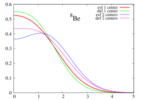
A more straight image of the modifications caused by the use of non-spherical harmonic oscillator functions for describing the movement of the nucleons can be provided by simply comparing the one-body density of the different distributions and approximations previosly presented. An average image of the spatial distribution of the nucleons comes from the radial one-body density, obtained after integrating in the angular degrees of freedom. In Figure 1, this radial density is shown for the nuclei: 8Be (left) and 12C (right) corresponding to the one-center and forming two and three -clusters, respectively. The radial density obtained for the two distributions of 8Be are quite different, specially the two -clusters in spherical approximation that present a depression around the center of mass. In both distributions, spherical approximation provides a more diffuse density than the non-spherical one. For 12C the same behavior appears; however, for this nucleus, all the densities present a depression around the center of mass. This depression is more important for the three -clusters distribution in spherical approximation and almost dissapears for non-spherical one-center distribution.
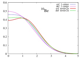
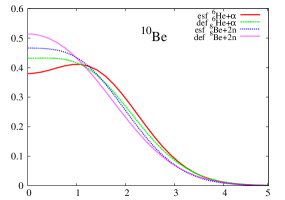
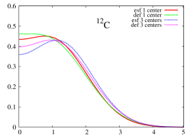
The radial one-body density for the proposed distributions for 10Be is shown in Figure 2. The behavior of the densities is roughly similar to the one discussed for the two previous nuclei, i.e., the spherical approximation provides more diffuse densities than the non-spherical one for the four analyzed distributions. If we compare the densities for the different distributions, we can see that differences increase with the degree of clusterization, that is, when we pass from one center, (1) to three centers (2) throught two centers: (3) and (4), in this order.
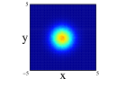
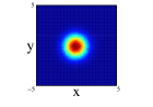


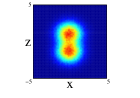
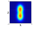
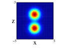
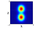
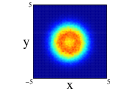
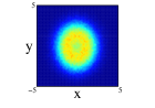
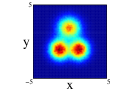
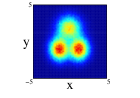
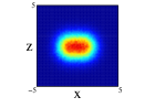
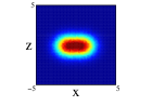
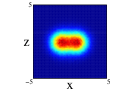
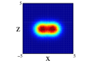
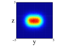
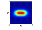
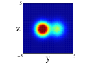
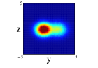
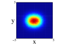
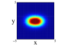
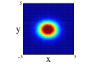
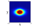
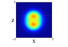
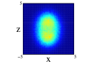
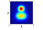
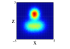
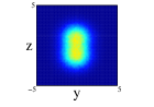
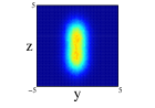
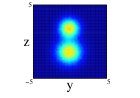
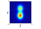
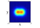
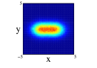
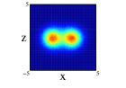
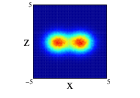
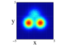
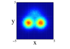
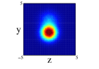
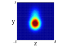
The angular average carried out for getting the radial one-body density does not allow to explore the spatial distributions of the nucleons since its intrinsic form is quite anisotropic for the studied distributions. A more adequate image is obtained if the projections of the spatial density on the three different cartesian planes is performed. This projections have been obtained by a Monte Carlo sampling of movements with an acceptance of for all the cases. For 8Be nucleus and due to the axial symmety around the -axis, the Figure 3 shows the projection on the plane (first row) and on the plane (second row) of the two distributions studied and with spherical and non-spherical approximations (see figure caption for further details). In the projections on the plane, we can see that the spherical approximation presents a more diffuse proyection than the non-spherical one for the two distributions. However, in the projection on , we can see that along the -axis, the diffusivity is more important in the non-spherical approximation compared to the spherical one and the behavior reverses on the -axis. These differences can not be appreciated in the averaged density since they compensate. In the two clusters distribution, an slight overlap between the clusters appears and it is more important for the non-spherical approximation. Finally, it is interesting to note that the nucleus is structured in two centers along -axis even in the case of only one cluster, although these two centers are not so well defined in the non-spherical approximation.
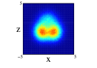
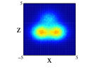
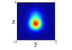
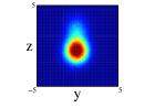
In Figure 4, we show for 12C nucleus, the projections on the three cartesian planes: (first row), (second row) and (third row) for the one center and three clusters forming an isosceles triangle distribution within spherical and non-spherical approximations (see caption for more explanations). For both distributions, we can see important difference between the two approximations. These are specially important in the plane for the one center case. For the three clusters distribution (whose centers define the plane) we can see the loss of the equilateral symmetry on the different projections on the and planes. This is also shown in the plane seeing the difference of diffusion of one of the centers (the one on the -axis) relative to the other two. Finally, to remark that the differences in the location of the nucleons are important as it can be infered from Figure 3, even though the radial density of both distributions is quite similar.
Finally we show the results for the 10Be nucleus. In Figure 5, we show the results of the projection for the four distributions in both approximations and on the three cartesian planes (see figure caption for further details). The locations of the two neutrons is quite clear for all the distributions except the one center case, (1), where appers as a diffuse halo in the and projections. It is interesting that clusterization is clear even in some of the distributions with an important part of the nucleons moving around the same center. The spatial locations of the nucleons are different for every of the distributions although there is an important resemblance between (2) and (4). Comparing for every distribution, the results between spherical and non-spherical approximations, there is a greater diffusivity in the non-spherical approximation in the different planes. However these differences almost disappear in the radial density after promediating in the angles.
7 Conclusions.
In the 10Be nucleus, the four spatial distributions studied are adequate candidates for describing the ground state. This suggests that a mixture of configurations with the four distributions could provide a better approximation to the experimental results.
Appendix: Multidimensional gaussian integral.
The integrals that appear in the calculation of matrix elements of the operators considered in this work, and that may involve one or more particles, can be written in general using cartesian coordinates as
| (12) |
with is a fixed vector in the –dimension space and is a non–singular matrix, usually non symmetric.
Everyone of these integrals can be determined by direct derivation respect to the components, of from the integral:
| (13) |
with is the inverse matrix of and its determinant. Derivating under the integral, it is easy to get that
| (14) |
Up to calculate all the integrals, we plan to establish a recurrence relation among them. For that, it is useful to define:
| (15) | |||||
| (16) |
Let us note that and independent of while depends linearly on so . Hereafter we shall write instead of . It is easy to get in the case when only the index is one and the rest are zeros that:
| (17) |
Taking this into account, we can write that:
| (18) |
and due to the mentioned properties of and , we can finally get that:
| (19) | |||||
This is the general recurrence relation that obliges to the index to be different from zero. A possible way of building all the integral is beginning with from to taking . After that taking first and increase from zero to and so forth to get for all the values of . We continue adding a new index different from zero that we take as value until we finally get to with .
Acknowledgments.
This work has been partially supported by the Spanish Dirección General de Investigación Científica y Técnica (DGICYT) under contract PB98–1318 and by the Junta de Andalucía.
References
- [1] J.A. Wheeler, Phys. Rev. 52, 1083 (1937).
- [2] H. Margenau, Phys. Rev. 59, 37 (1941).
- [3] J.J. Griffin and J.A. Wheeler, Phys. Rev. 108, 311 (1957).
- [4] D.M. Brink, in: Proc. Int. School of Physics, Enrico Fermi 36, Academic Press, New York, p. 247 (1966).
- [5] D.M. Brink and A Weiguny: Nucl. Phys. A120, 59 (1968).
- [6] Y. Abe, J. Hiura and H. Tanaka, Prog. Theor. Phys. 49, 800 (1973).
- [7] Y. Kanada-En’yo, H. Horiuchi, and A. Ono, Phys. Rev. C52, 628 (1995).
- [8] P. Descouvemont and M. Dufour, Nucl. Phys. A621, C311 (1997).
- [9] M. Dufour and P. Descouvemont, Phys. Rev. C56, 1831 (1997); Nucl. Phys. A726, 53 (2003).
- [10] Y. Kanada-En’yo and H. Horiuchi, Phys. Rev. C52, 647 (1995).
- [11] Y. Kanada-En’yo, H. Horiuchi and A Doté, Phys. Rev. C60, 064304 (1999).
- [12] Y. Kanada-En’yo and H. Horiuchi, Phys. Rev. C66, 024305 (2002).
- [13] Q.K.K. Liu, H. Kanada and Y.C. Tang, Phys. Rev. C23, 645 (1981).
- [14] P. Descouvemont, Phys. Rev. C70, 065802 (2004).
- [15] M. Dufour and P. Descouvemont, Phys. Rev. C78, 015808 (2008).
- [16] P. Descouvemont and M. Dufour, ’Microscopic Cluster Models’ pags 1-66, in ’Cluster in Nuclei, Vol.2’ edited by C. Beck, Lectures Notes in Physics 848, Springer-Verlag (2012).
- [17] W. von Oertzen, M. Freer, Y. Kanada-En’yo, Phys. Rep. 432, 43 (2006)
- [18] M. Dufour and P. Descouvemont, Nucl. Phys. A605, 160 (1996).
- [19] J.M. Eisenberg and W. Greiner, Nuclear Theory, Volume 1: Nuclear Models, Third edition, North Holland (1988)
- [20] A. B. Volkov, Nucl. Phys. 74, 33 (1965).
- [21] D. Brink and E. Boeker, Nucl. Phys. 91, 1 (1967).
- [22] D. R. Thomson, M. Lemere and Y. C. Tang, Nucl. Phys. A286, 53 (1977).
- [23] P. Descouvemont, Nucl. Phys. A699, 463 (2002).