MIT-CTP-4629
Non-toric bases for elliptic Calabi-Yau threefolds and 6D F-theory vacua
Abstract
We develop a combinatorial approach to the construction of general smooth compact base surfaces that support elliptic Calabi-Yau threefolds. This extends previous analyses that have relied on toric or semi-toric structure. The resulting algorithm is used to construct all classes of such base surfaces with and all base surfaces over which there is an elliptically fibered Calabi-Yau threefold with Hodge number . These two sets can be used to describe all 6D F-theory models that have fewer than seven tensor multiplets or more than 150 neutral scalar fields respectively in their maximally Higgsed phase. Technical challenges to constructing the complete list of base surfaces for all Hodge numbers are discussed.
1 Introduction
The problem of classifying Calabi-Yau threefolds is important both for mathematics and for physics. In mathematics, progress in recent years on the minimal model program for surfaces and for higher-dimensional algebraic varieties (i.e. Mori theory Mori ) has provided tools for understanding and classifying threefolds and higher-dimensional varieties with non-vanishing canonical class. These methods are not directly applicable, however, to classification of Calabi-Yau manifolds, which have a canonical class that vanishes (up to torsion). In physics, Calabi-Yau manifolds play an important role as compactification spaces for string theory chsw . Classification of Calabi-Yau manifolds is useful in understanding the space of vacuum solutions of string theory. Despite many years of study of these spaces, it is still not known if the number of distinct topological types of Calabi-Yau threefolds is finite or infinite. Physicists have systematically analyzed certain types of Calabi-Yau manifolds using specific constructions such as complete intersections in projective spaces (CICY’s CICY ) or hypersurfaces in toric varieties Batyrev . A particularly useful compilation of data for the full set of toric hypersurface Calabi-Yau’s was made by Kreuzer and Skarke Kreuzer-Skarke (see also CY-data-2 for more refined data for the threefolds with small , and CY-explorer for a nice graphical interface to the set of current Calabi-Yau data.). See Davies ; He for recent reviews of various approaches to constructing and classifying Calabi-Yau threefolds.
The space of elliptically fibered Calabi-Yau threefolds represents a subset of the set of Calabi-Yau manifolds that is known to admit a finite number of topological types Gross . In recent years, motivated by the physics of F-theory F-theory ; Morrison-Vafa-I ; Morrison-Vafa-II , a systematic approach has been developed to classifying elliptically fibered Calabi-Yau threefolds through the geometry of the base of the elliptic fibration, which is a complex surface. The set of possible configurations of mutually intersecting curves of self-intersection or below that can arise on a surface supporting an elliptic fibration where the total space is Calabi-Yau were classified in Classbasis . These “non-Higgsable clusters” provide building blocks out of which all base surfaces that support elliptic Calabi-Yau threefolds can be constructed. The complete set of allowed compact toric bases was described and enumerated in Toric ; this analysis was extended to bases with a single -structure in semi-toric . For each allowed base, there are many possible different elliptic Calabi-Yau manifolds over that base; each distinct topology can be realized by resolving singular geometries constructed by “tuning” coefficients in a generic Weierstrass model over the given base (see, e.g., JohnsonTaylor ) to realize different Kodaira singularity types over divisors in the base. Non-Higgsable clusters have also been used as basic building blocks in the construction of general 6D superconformal field theories SCFT-1 ; SCFT-2 ; SCFT-3 .
In this paper we develop methodology to classify general smooth compact bases that support elliptic Calabi-Yau threefolds, without restricting to base surfaces with toric or any other specific structure. The approach we take is combinatorial in nature. From the minimal model program for surfaces bhpv and the work of Grassi Grassi it is known that all allowed bases can be formed from blow-ups of the Hirzebruch surfaces , projective space , or the Enriques surface. Our basic approach is to characterize each surface in terms of the combinatorics of the cone of effective curves. This data can be characterized by the set of vectors that generate the effective cone in the lattice , where corresponds to the number of tensor multiplets in an F-theory compactification on the base surface . In most cases, the cone has a finite number of generators and this is a finite combinatorial problem.
There are a number of technical complications that can arise in this analysis. In some cases, the number of generators of the effective cone can become infinite. In other situations, the combinatorial structure of the cone of effective curves is insufficient to uniquely specify the geometry of the base surface. In this paper we describe these complications and develop an algorithm for explicitly constructing bases that avoids these issues in some regions of interest. This gives a systematic approach to constructing large classes of bases for elliptic Calabi-Yau threefolds. In particular, we construct bases with small , and bases that give generic elliptic fibrations corresponding to Calabi-Yau threefolds with Hodge number . In both cases, we believe that we have constructed all possible bases in the appropriate regime, though we have not proven this in a completely rigorous mathematical fashion. In principle, a systematic analysis of tuning Weierstrass moduli over these bases could lead to a systematic construction of all elliptic Calabi-Yau threefolds with large or small .
In §2, we review the basics of F-theory and the connections between the geometry of a complex base surface , the generic elliptic Calabi-Yau threefold over , and the physics of the corresponding F-theory compactification. We also review some basic complex algebraic geometry of surfaces. In §3, we give some very simple examples of base surfaces and the structure of the cone of effective curves on these bases. In §4, we describe in some detail how the cone of effective curves can be determined when a surface is formed as the blow-up of another surface. We describe a more general class of examples, the generalized del Pezzo surfaces, in §5. In §6 and §7, we discuss obstructions to the systematic combinatorial construction of all base surfaces. In §8 we describe the systematic algorithm for classification of bases, and give the results of applying the algorithm for small in §9 and for large in §10. Some concluding remarks are given in §11
Note that while the analysis in this paper is carried out in a concrete mathematical framework, we have not attempted to be completely rigorous from the mathematical point of view. The goal of this work is to explore the space of general bases that support elliptic CY threefolds using a combinatorial and algorithmic approach that gives insight into the nature of the scope and structure of generic bases of this type. In various places in the paper we point out some specific ways in which our analysis neglects certain complexities which would need to be addressed more systematically for a complete classification of all bases supporting elliptic CY threefolds with arbitrary Hodge numbers.
2 Complex surfaces as F-theory bases
We summarize here some basic facts from the physics of F-theory and the algebraic geometry of complex surfaces. For a more detailed introduction to F-theory, see the reviews Morrison-TASI ; Denef-F-theory ; WT-TASI .
2.1 F-theory on elliptic Calabi-Yau threefolds
When F-theory is compactified on a compact Calabi-Yau threefold that is elliptically fibered, one gets a 6D theory of gravity with supersymmetry. This theory may also contain tensor, vector, and scalar (hypermultiplet) fields.
The elliptic fibration must have a global section; a Weierstrass model of any such fibration exists Nakayama and takes the form
| (1) |
If we denote the canonical class of the base by , then the functions , and are sections of line bundles , and respectively.
The fiber is singular along loci in the base manifold where the discriminant
| (2) |
vanishes. The Kodaira-Tate classification characterizes codimension-one singularities where the discriminant vanishes Kodaira ; Tate . When the functions , and vanish to specific orders on a divisor , the singularity is associated with the Dynkin diagram of a certain non-Abelian gauge algebra that describes a gauge field in the corresponding physical 6D supergravity theory Morrison-Vafa-I ; Morrison-Vafa-II ; Bershadsky-all ; Morrison-sn ; Grassi-Morrison-2 . The correspondence between vanishing orders of and nonabelian symmetry algebras is listed in Table 1. Codimension two singularities give rise to matter fields in the 6D theory, though this correspondence is not yet completely classified. Note that if vanish to order or higher at a codimension-one locus on the base, the singular Weierstrass model (1) cannot be resolved into a smooth Calabi-Yau threefold. Then the F-theory compactification does not have a supersymmetric M-theory dual, hence it will not give any supergravity vacua. These points are also at infinite distance in the Weierstrass moduli space. If vanishes to order or higher at a codimension-two locus (points) on the base, then such points need to be blown up on the base in the resolution process to give a smooth Calabi-Yau threefold.
| Type | ord () | ord () | ord () | sing. | symmetry algebra |
|---|---|---|---|---|---|
| 0 | 0 | 0 | none | none | |
| 0 | 0 | or | |||
| 1 | 2 | none | none | ||
| 1 | 3 | ||||
| 2 | 4 | or | |||
| or or | |||||
| 2 | 3 | or | |||
| 4 | 8 | or | |||
| 3 | 9 | ||||
| 5 | 10 | ||||
| non-min | does not appear for SUSY vacua | ||||
Rational curves of negative self-intersection on the base surface can enforce minimal degrees of vanishing of , , over those curves, for a generic elliptic fibration. When this happens, the physical theory has some minimal content of gauge fields and matter fields, regardless of the specific fibration one chooses in the Weierstrass moduli space. The configurations of curves of negative self-intersection that give rise to gauge and matter fields in this way were classified in Classbasis , and dubbed “non-Higgsable clusters” (NHCs), since the 6D gauge groups that arise in this way cannot be broken in a fashion that preserves supersymmetry by giving vacuum expectation values to (i.e., “Higgsing”) the charged matter fields. We have listed the configurations of possible NHCs in Table 2. While the gauge groups produced by non-Higgsable clusters cannot be broken in any supersymmetric vacuum without changing the base , the coefficients of the Weierstrass model, associated with neutral scalar fields in the 6D supergravity theory, may be tuned to enhance the gauge contents of the theory. It was shown, for example, that in this way all elliptically fibered Calabi-Yau threefolds with (and indeed all known Calabi-Yau threefolds exceeding this Hodge number bound) can be constructed through tuning Weierstrass models over simple complex base surfaces JohnsonTaylor .
| Cluster | gauge algebra | |||
|---|---|---|---|---|
| (-12) | 8 | 248 | 0 | |
| (-8) | 7 | 133 | 0 | |
| (-7) | 7 | 133 | 28 | |
| (-6) | 6 | 78 | 0 | |
| (-5) | 4 | 52 | 0 | |
| (-4) | 4 | 28 | 0 | |
| (-3, -2, -2) | 3 | 17 | 8 | |
| (-3, -2) | 3 | 17 | 8 | |
| (-3) | 2 | 8 | 0 | |
| (-2, -3, -2) | 5 | 27 | 16 | |
| (-2, -2, …, -2) | no gauge group | 0 | 0 | 0 |
The Hodge numbers of the generic (i.e., untuned) elliptic Calabi-Yau threefold associated to a given base can be easily computed from the non-Higgsable cluster content of the base WT-Hodge using the relations
| (3) | |||
| (4) |
Here, as above, is the number of tensor multiplets. The quantity is the total rank of (nonabelian + abelian) gauge groups. and are the numbers of 6D vector supermultiplets and charged matter hypermultiplets respectively Morrison-Vafa-I ; Morrison-Vafa-II . , , and the contribution of nonabelian gauge groups to can be directly computed by summing up the contributions of all NHCs, using Table 2, when the intersection structure of curves on the base is known. In principle, there can also be an abelian contribution to , even when is the generic elliptic CY threefold over the base . While this does not occur for toric base surfaces , it was found in semi-toric that there are a small number of base surfaces with a single structure (“semi-toric” bases) that give rise to theories with a non-Higgsable abelian gauge group structure. The corresponding Calabi-Yau threefolds are elliptic fibrations with multiple independent sections, corresponding to a higher rank Mordell-Weil group. It is shown in Morrison-Park-Taylor that all these threefolds are related and can be described through a generalization of the Schoen construction Schoen . In general, computing the rank of the Mordell-Weil group for a given compactification space is a difficult mathematical problem, which we do not attempt to address here. For the specific classes of non-toric bases that we enumerate here, there are no abelian contributions to for generic elliptic fibrations. For a comprehensive analysis of bases giving elliptic Calabi-Yau threefolds with large and small , however, this possibility would need to be considered further.
As mentioned above, the base of any elliptically fibered Calabi-Yau threefold can be constructed by blowing up a finite number of points on , a Hirzebruch surface or the Enriques surface. The F-theory models in the case of the Enriques surface are relatively trivial, and do not allow any gauge field or matter content, since vanishes (up to torsion). In this paper we only consider and Classbasis . In Kodaira’s classification of complex surfaces (not to be confused with his classification of codimension one singularities in elliptic fibers mentioned above), these are all rational surfaces (birational to ), with Kodaira dimension bhpv . The condition that have global sections means that the anticanonical class is in the cone of effective divisors. Stated more technically, the complex surfaces we study in this paper are anticanonical rational surfaces Looijenga ; Harbourne1997 , or those where the anticanonical class is an effective -divisor. We focus in this paper only on smooth base surfaces .
2.2 Algebraic geometry of rational complex surfaces
The general theory of complex algebraic surfaces can be found in Griffith-Harris ; bhpv . We review here a few basic definitions and ideas that will be helpful in systematically generating base surfaces.
A (Weil) divisor is a formal linear combination with integer coefficients of irreducible algebraic curves on the algebraic surface . If the coefficients in the linear combination are all non-negative, then the divisor is effective, . A -divisor is defined similarly to a Weil divisor, but with coefficients in (Note that Weil divisors and Cartier divisors coincide on smooth varieties, which is the only situation that we consider here). The divisor class is the homology class of . The set of divisor classes modulo linear equivalence on forms an additive group, which is homomorphic to the Picard group Pic of line bundles on the surface (which form a group under the tensor product operation). For effective divisors, the divisors in the same divisor class as a given divisor are said to be linearly equivalent, and form a linear system, denoted .
There is a bilinear operation PicPic, which corresponds to the intersection number of two divisor classes. For two distinct divisor classes , we can pick out one specific representative from each class; the intersection number then just coincides with the geometric number of intersection points (with multiplicity) between the two curves and . The self-intersection of a divisor class is . Note that the self-intersection of a curve can be negative, but only when the curve is rigid and cannot be deformed; otherwise a small deformation would give two distinct curves that would intersect at a finite positive number of points. (because of the complex structure, all intersections between complex curves in a surface have the same orientation, and all contribute positively to intersection numbers.)
For , the inequivalent divisor classes are those of the form , where and is the divisor class of the hyperplane in ; the hyperplane is just a line given by a linear equation, for example as described by the algebraic equation in homogeneous coordinates on . The linear system corresponds to the space of all degree- curves on .
The mathematical procedure of blowing up a point on a smooth surface consists of replacing the point by a copy of , called the exceptional curve, where the points on the correspond to all (complex) directions in which lines on the original surface can pass through the original point. After a blow-up process, a new effective divisor class arises on the resulting blown up surface , which is the class of the exceptional curve . This divisor class has self-intersection ; the linear system of the exceptional curve only contains one curve, hence it is generally just called the exceptional curve. There is a birational map , which is one-to-one and onto everywhere except on the exceptional curve, where and is the point being blown up. If there is some representative curve of a certain effective divisor class that passes through the point , with multiplicity , then after the blow-up process, a new divisor class
| (5) |
appears as an effective divisor class on . This is called the proper transform of . Here we have identified on with .
For a given surface generated by blowing up consecutively times, a convenient basis of Pic consists of the divisor class of the hyperplane on the original and the exceptional divisors . The intersection matrix on this basis is given by
| (6) |
Hence the Picard rank is rk(Pic.
More generally, the Hodge index theorem states that for any surface with rk(Pic) , the signature of the intersection matrix is . When , there is always a basis in which the intersection product takes the form (6); for , there are surfaces where the intersection form has the structure of the matrix
| (7) |
The canonical divisor class of is , and after blow-ups is always in the form of
| (8) |
More generally, the canonical divisor class can always be taken to have this form in a basis with intersection form (6). In general, if an irreducible divisor class on a surface formed from blow-ups on can be decomposed into a sum of the hyperplane and other divisor classes as , then it is the divisor class of some degree curve on the original .
There is a useful genus formula that follows from the adjunction formula:
| (9) |
where is the genus of the curve . If , then is a rational curve. If , then is an elliptic curve. Note that the anticanonical divisor class is always elliptic.
The dimension of the linear system is related to the dimension of the cohomology class of sheaves :
| (10) |
For rational curves , we have the following result from the Riemann-Roch theorem Kollar ; CaporasoHarris ; CaporasoHarris2
| (11) |
If , then there exists a curve that passes through general points. This implies furthermore that if for another divisor class , then for every generic point on , there exists a curve that passes through it. This is the case whenever the class of the divisor has non-negative self-intersection. When the class has negative self-intersection, then , which means that the curve in cannot be deformed. In this case, if is irreducible, then it is really a single “fixed” curve.
For general (arbitrary genus) curves, the value of satisfies Griffith-Harris .
In general we have the following lemma:
Lemma 1.
A negative divisor class on is always rigid. For a non-negative effective divisor class on , there exists a representative that passes through any points in .
More generally, this lemma also guarantees that curves of sufficiently positive self-intersection can pass through points with arbitrary multiplicity. When , for example, there is a representative curve that passes through any point in with multiplicity 2 (which requires two additional conditions, corresponding to the vanishing of the two first derivatives at ). In general, for a curve to exist that passes through any point with multiplicity , we must have .
Note that the above statements are completely consistent with the intuition of planar geometry. For example, consider the curves of self-intersection on a surface formed by blowing up times. The divisor classes of degree 1 rational curves with self-intersection can be written as , corresponding to the set of lines that pass through the pairs of points and on the original . There is a unique line that passes through two fixed points in the plane, hence the resulting -curve is fixed. Similarly, the divisor class of degree 2 rational curves with self-intersection can be written as , corresponding to the set of conics that pass through five fixed points. We know this divisor is also rigid, since there is a unique conic passing through five fixed points. If we consider, however, the divisor class of degree 1 rational curves with self-intersection 0, , these correspond to the set of lines that pass through a particular point , and are free to move. In fact, such lines can pass through through every point on .
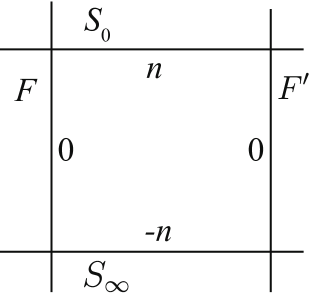
We have focused so far on blow-ups of , but the above properties of divisors can also be applied to the Hirzebruch surfaces (Note that is the surface that results from blowing up a single point on ). In the language of toric geometry, the irreducible toric divisors form a cyclic diagram (see Figure 1). For the cases with odd , the relevant divisor classes can be written in the basis (6) using the following linear combinations of the two generators of Pic:
| (12) |
The canonical class is, for all ,
| (13) |
The blowing-up of at points has the same Picard groups and intersection matrices for each , and matches with that of blown up at points. Also, the canonical class is always again in the form . Generally speaking, therefore, although the geometric intuition comes most easily from , the structure of divisors and intersection structure is essentially the same on other rational surfaces arising as blowups of Hirzebruch surfaces.
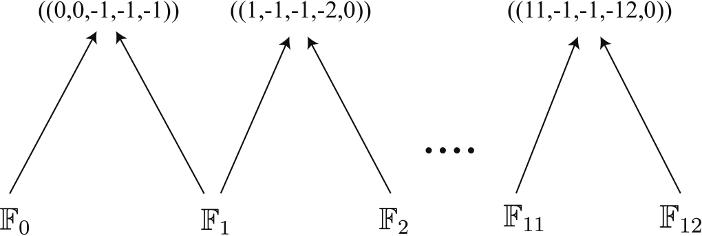
For even , we can relate any blow-up of the Hirzebruch surface to the cases with odd via the blow-up chains shown in Figure 2. Thus, every surface that results from blowing up can be generated by blowing up or . Hence, to enumerate all possible base surfaces with that support elliptic Calabi-Yau threefolds we only need to take with odd as starting points for the blowing up process.
The set of effective divisor classes on forms a cone, called the effective cone Eff. The dual of the effective cone is the set of divisor classes that intersect non-negatively with Eff; this is called the nef cone Nef:
| (14) |
Elements of the nef cone are called nef divisors (classes). In general, an element in the effective cone need not be nef; for example, any effective divisor of negative self-intersection is not nef. Conversely, however (see e.g. Corollary II.3 in Harbourne1997 ), any nef divisor class on a smooth rational surface is effective.
The effective cone is the primary distinguishing characteristic of different rational surfaces. For example, the Hirzebruch surfaces with odd all have the same intersection form as discussed above. The cone of effective divisors, however, is generated by and , and is different for each .
Our primary tool in this paper for studying base surfaces will be the combinatorial structure of the effective cone. The following result, which is Proposition 1.1 in Cox-rings , will be useful
Lemma 2.
For surfaces generated by blowing up , which have Picard rank greater than 2, when the effective cone is polyhedral (i.e. generated by a finite set of vectors), then the effective cone is generated by rational divisor classes with negative self-intersection.
For the Hirzebruch surfaces, of Picard rank 2, it follows directly from the explicit description above that the effective cone is generated by rational divisor classes with non-positive self-intersection (i.e., , where for ). After one blow-up, Lemma 2 applies. Blowing up ( odd), an effective class with self-intersection always appears. Then the effective class with 0 self-intersection can be written as a non-negative linear combination of and exceptional divisors. This property generally holds for surfaces with higher Picard rank.
We discuss these statements further in section 4.
Note that curves of negative self-intersection on a base surface that supports an elliptic Calabi-Yau must always be rational. From (9), an irreducible curve of negative self-intersection with satisfies . From this it follows that contains at least times. This means that must vanish to at least orders over so we cannot have such a curve in a base that supports an elliptic Calabi-Yau threefold.
To close this section, we introduce some terminology that we will use frequently in the remainder of the paper.
-
•
In general we will not distinguish between “divisor class”, “divisor” and “curves”. Thus, for example, the divisor class is generally written as . When we talk about “-curves”, this refers to a divisor class with self-intersection . We often use the term “negative curve” to refer to a curve of negative self-intersection.
-
•
Following Lemma 2 and the subsequent discussion, the negative curves that appear in the surfaces in which we are interested in are always rational. Furthermore, in the cases where Lemma 2 applies, we define Neg as the set of irreducible negative rational curves that generate Eff. A general requirement for Neg is:
For , if , then . This is just the statement that two different irreducible curves cannot intersect each other negatively.
-
•
We further define the set of irreducible rational curves with self intersection number less than -1 to be Sing. These include the non-Higgsable clusters described in Table 2, as well as configurations of -curves whose intersection matrices are exactly the Cartan matrices for ADE Lie algebras.
-
•
When discussing toric bases, we indicate the cycle of self-intersection numbers by e.g. .
-
•
We will use the vector representation for the divisor class . This applies to surfaces that arise from blowing up any any number of times.
-
•
We define the set of genus , self-intersection divisors that intersect non-negatively with every curve by . They are all effective curves, as we mentioned before. All such curves can be described as integer vectors as described in the previous point.
Finally we define .
-
•
Using the terminology in Derenthal ; DerenthalThesis , for two surfaces and , if there is a bijection between Neg and Neg that preserves the intersection structure then Eff and Eff are isomorphic, and we say that and are “of the same type”. This equivalence relation is weaker than isomorphism, as demonstrated in DerenthalThesis . Nevertheless, two surfaces of the same type give the same minimal gauge algebra. The blow-up descendants of two surfaces of the same type may be different, as will be discussed in section 5.
-
•
We always denote the one-time blow-up of the surface by
3 The general strategy and some simple examples
Given the basic background and definitions from the previous section, we can now outline the strategy we will use for constructing bases. The idea is to keep track only of the combinatorial information associated with the generators of the effective cone. While this loses some information – in particular it does not distinguish surfaces of the same type that are not isomorphic – it gives us a simple combinatorial handle on a large class of surfaces.
Assume that we are given the information about the generators of the effective cone for a given surface . According to Lemma 2, this will generally be a finite set of curves of negative self-intersection. We can then attempt to construct all blow-ups of by considering all combinatorial possibilities consistent with the geometric structure of the effective cone. In many cases this is straightforward. The point that is blown up can either lie on one of the negative curves that is a generator of the effective cone, or on an intersection of such negative curves, or on a more general point. Lemma 1 can be used to determine which curves on the surface can pass through the point , and this information in principle can be used to determine the structure of the effective cone for the blown up surface .
While this approach works in many situations in an unambiguous fashion, there are various situations in which complications arise. Such complications can include the appearance of an infinite number of generators for the effective cone, or a situation as mentioned above where there are non-isomorphic surfaces of the same type. We discuss these issues in more detail later in the paper. Here we give a few examples of how the combinatorial data describes the effective cone and blow-ups in some simple cases where there are no complications. These examples serve as illustrations of the general ideas described in the previous section, and clarify the nature of the computational problem in generalizing the construction to arbitrary surfaces.
Let us begin with the base . The intersection form on this base is positive definite, with generator having . The divisor class of , corresponding to a line on , is a generator of the effective cone. From (3, 4), it is straightforward to determine that the Hodge numbers of the generic elliptic fibration over are , since .
Now consider a single blow-up of at a generic point . There is a line on that passes through any point (a trivial application of Lemma 1). Thus, the generators of the effective cone for the new surface are
| (15) | |||||
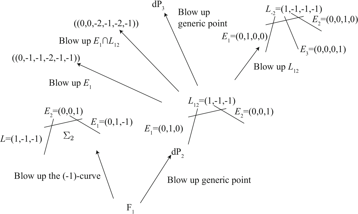
where the subscript on the divisor class denotes the self-intersection of that curve. This is, of course, the Hirzebruch surface as described above, also known as the del Pezzo surface ; in general, the del Pezzo surface is constructed by blowing up at independent points. The base has a toric description, with a cyclic set of toric divisors having self-intersections . The generic elliptic fibration over this base has Hodge numbers , since .
Now, we consider possible blow-ups of the surface . There are only two distinct types of blow-up, from the point of view of the combinatorics of the effective cone. We can blow up at a point on the curve , or we can blow up at a generic point. These two types of blow-ups result in the following surfaces:
Blowing up at a generic point that is not on the curve gives a new effective cone generated by three curves
| (16) | |||||
| (17) | |||||
| (18) |
This surface is also known as . Note that the line in has self-intersection 0, so by Lemma 1 will pass through any point, including the point ; this guarantees the existence of the curve , which corresponds in the original to the line passing through the two points that are blown up to get this surface.
Blowing up at a point on the curve gives a new effective cone generated by two curves and a curve
| (19) | |||||
| (20) | |||||
| (21) |
The fact that the line on is in a linear system of dimension 1, and can be chosen to pass through , follows again from Lemma 1. We refer to the resulting surface as .
Note that the two distinct blow-ups of to and correspond to the two branches above in Figure 2. Each of these two surfaces has a toric description. The fact that in each of these cases the set of generators of the effective cone consists completely of curves of negative self intersection is a consequence of Lemma 2. Both of these surfaces support generic elliptic Calabi-Yau threefolds with Hodge numbers .
We can continue in this fashion. There are four combinatorially distinct ways to blow up the surface , corresponding to blow-ups on , and a generic point.
Blowing up at a generic point gives . The effective cone for has six generators, corresponding to the 3 exceptional divisors and the 3 lines . This illustrates one of the main challenges of doing this combinatorial blow-up construction systematically: it is necessary at each step to identify all possible new curves of negative self-intersection that can be produced at each stage of the blow-up process. Addressing this challenge is the primary goal of the following section.
Three of the four ways in which can be blown up have a toric description; blowing up at , and a generic point respectively give toric bases with a cyclic set of effective toric divisors having self-intersections and . (The last of these is ). The final possibility, blowing up at a point in gives a non-toric base with the following generators for the effective cone
| (22) | |||||
| (23) | |||||
| (24) | |||||
| (25) |
Similarly, there are 6 combinatorially distinct ways of blowing up the surface ; 5 of these correspond to toric constructions, and the sixth, associated with blowing up on the curve , gives another non-toric base. Of the toric bases, two involve blowing up a point on the curve, giving a curve. While the other bases support elliptic Calabi-Yau threefolds with Hodge numbers , the two with curves support elliptic Calabi-Yau threefolds with Hodge numbers , since there is a non-Higgsable cluster with .
Continuing in this fashion, we can construct a wide range of types of complex surfaces that support elliptic Calabi-Yau threefolds. At each stage it is necessary to determine the complete set of curves of negative self-intersection that generate the effective cone. Dealing with this computation is the subject of the next section.
4 Identifying new curves after a blow-up
In this section we describe the different types of points that can be blown up in passing from one surface to another . We then describe an algorithm to compute all curves that generate the effective cone in finite time.
4.1 Types of blowups
As mentioned before, when we blow up a point that lies with multiplicity on a representative of an effective divisor class and self-intersection , there is a new effective divisor class , written in the vector representation. Using the Riemann-Roch formula (9), the following lemma holds:
Lemma 3.
If one blows up a curve at an -point on , the resulting new effective curve on is: .
This implies that blowing up a single point on a curve will not change its (arithmetic) genus, but blowing up an -point on a curve will decrease the genus of the curve by .
Then given a base , the different ways of blowing it up can be classified as follows:
(1) One can blow up a generic point on . Then all the elements Neg are transformed to , because they are fixed and they will not pass through a generic point . The exceptional curve is an element in Neg that is a generator of the new effective cone. In order to construct the full Neg that generates Eff, we also need to blow up all the elements at a single point, blow up all the elements at a double point, blow up all the elements at a triple point, and so on…This process can always be done in principle due to Lemma 1. In the next subsection we describe how this can be realized in practice with a finite amount of computation.
As a consistency requirement, the resulting rational curves after the blow up should intersect non-negatively with each other. This is equivalent to the following statement:
For , that are blown up in this process, ().
(2) One can choose to blow up a non-generic point, so that a set of curves are blown up at a single point. The index here just labels different curves with same genus. In the simplest cases, the point blown up lies only on a single rational curve of negative self-intersection, in which case the transformed curve is . The point blown up may also lie at an intersection point between a pair of negative curves , in which case both curves are transformed and .
(3) There are also situations where a set of curves are blown up at a double point, are blown at a triple point, and so on. This will produce new negative rational curves of self-intersection that must be included in Neg We define the blow-up process to be a “special blow-up” when one or more (-2) or lower curves are generated by blowing up positive curves at points with multiplicity higher than 1.
(4) In some cases it may be possible to choose a non-generic point as in (2) that lies at the intersection of more than two negative curves.
Cases (1) and (2) can be handled in a systematic fashion using the combinatorial data of the effective cone. Case (3) may or may not give us new bases. In the specific regimes that are thoroughly studied in this paper, special blow-ups are observed not to occur. Case (4) is discussed further in section 6, and also does not occur in the regimes that we study explicitly.
Just as for blowups producing curves, we require that for intersecting curves , , that are blown up at points of multiplicity respectively, we must have . Otherwise after the blow up, Neg will contain two different elements that intersect each other negatively.
4.2 Generating the set of -curves on
From the analysis above, all the curves in the set Sing can be generated by blowing up non-generic points. However, there is also in general a new set of (-1)-curves in Neg, and it is not clear whether the algorithm generating (-1)-curves described above is finite or not. In principle we need to look at all the sets , but this is impossible to do. Now we prove a powerful proposition, which contains the methodology to generate all the -curves with a finite amount of work:
Proposition 1.
The set of rational (-1)-curves generated by the blow up method is the solution set to the following Diophantine equations:
| (26) |
with the additional requirement that the curve intersects non-negatively with all the elements in Sing.
Actually the two equations are nothing but the defining equations of self-intersection and genus.
Proof.
We prove this by induction. First one can check the correctness of this statement for and . Then suppose this is true for a base ; we want to show this is also true for any surface that is generated by blowing up once.
(i) All the curves satisfy the requirements in the proposition.
Obviously they satisfy the Diophantine equations. If negatively intersects with Sing, this means where is some other effective divisor, hence is reducible and is not in Neg.
(ii) All the irreducible rational (-1)-curves that satisfy the non-negative intersection requirement in the proposition are elements of , and can be generated by the blow-up process. We analyze the different types of solution to (26) separately.
(a) This is obviously true for the solution since it is the exceptional curve associated with the blowup , and none of the other curves has a positive last entry.
(b) For all the solutions of the form , where we know that intersects non-negatively with all the elements in Sing, it follows by induction that . From the general characterization of the blow-up process described earlier, is still in Eff, but it may be represented as a positive linear combination of a lower self-intersection effective curve and the exceptional curve: . When this happens, however, it means that intersects negatively with Sing, which contradicts the requirement in the proposition. Hence is irreducible when it satisfies the requirement in proposition, and it is in .
(c) For all the solutions of the form , , is a genus , self intersection divisor. In fact the solution to the equations (26) automatically intersects non-negatively with any other solutions (see Theorem 2a in Nagata ). Together with the assumption that intersects non-negatively with all the elements in Sing, we can conclude that intersects non-negatively with any other curve in Neg. From this we can also know that is nef hence is effective on . Then according to Lemma 1, can be blown up at a generic point with multiplicity . These statements together guarantee that is an irreducible curve on . Hence any solution of the form , that satisfies the requirement in the proposition is in Neg. ∎
Actually, it is known that Proposition 1 holds for generalized del Pezzo surfaces Derenthal ; DerenthalThesis . We just needed to confirm that it holds for the bases that we are interested in.
Now the question is how to generate the solutions to the Diophantine equations using a finite algorithm. In fact, all the solutions can be generated by a series of “-operations” acting on curves, which are defined as follows Nagata :
For a curve in the form , one picks three numbers out of , then performs the following transformation:
| (27) |
It can be explicitly checked that the two quantities and do not change under this transformation. In fact, this operation is the Cremona transformation with center .
In practice, one starts from some low-degree curves, such as all the degree 0 and degree 1 rational (-1)-curves. Then one tries to perform all the -operations on one curve so that the degree is increased ( in (27) ). If the curve intersects negatively with some element in Sing, then we cut this branch. This recursive algorithm is finite if Eff is finitely generated. We discuss more about the finiteness of curves in section 6.
There are some cases, however, where a high degree (-1)-curve exists but there are no valid degree 1 curves. If this happens, the set of (-1)-curves we get from the recursive algorithm above is not complete. This is equivalent to the statement that there is another (-1) curve that intersects non-negatively with all the curves we have found, but it is not in the solution set generated by carrying out the algorithm up to a fixed degree . Such an additional curve would appear to be a negative curve in the nef cone, which is impossible. While the full set of (-1)-curves would in principle be produced by keeping all intermediate branches and continuing the algorithm to arbitrary , without some further check on the completeness of the set of generators for the effective cone we would not have a means of terminating the algorithm. So for a consistency check we compute the dual cone of Neg generated by the method above, and check that the generators (extremal rays) of this dual cone are non-negative. If a generator is negative, we know it is a (-1)-curve in Neg that was not generated by the -process. After adding all the (-1)-curves of this kind, we can get a complete set of curves in Neg, with a dual cone that contains no negative curves.
Another more complicated issue is the “special blow-up” that was defined earlier, where one blows up a non-generic point on a curve with genus higher than 1 to get an element in Sing. This also appears to make the algorithm infinite, since in principle we need to examine the set of all positive curves. This issue appears to be difficult to handle in a completely general context, and we will discuss this issue in specific regimes.
5 Working example: (generalized) del Pezzo surfaces
As a simple set of examples we now consider the class of surfaces called del Pezzo surfaces and generalized del Pezzo surfaces. The definition and basic properties of these objects can be found in Derenthal .
A generalized del Pezzo surface is a non-singular projective surface whose anticanonical class satisfies and for all effective divisors on the surface.
Any generalized del Pezzo surface is isomorphic to , , or the blow up of in points in almost general position. The degree of the generalized del Pezzo surface is given by . The phrase “almost general position” means that the surface does not contain curves of self-intersection or below, which implies that it does not contain any NHCs and there is no minimal gauge content in the corresponding low-energy 6D supergravity theory.
If a generalized del Pezzo surface does not contain any (-2)-curves, then it is just an ordinary del Pezzo surface, which is , , or the blow up of in points in general position. By general position, one requires that no three points in lie on a line, no six points lie on a conic and no eight points lie on a cubic with one of them a double point on that curve. This is equivalent to the statement that none of the points being blown up is a point on a (-1)-curve or a double point on a 2-curve, which would result in (-2)-curves. We define the del Pezzo surface to be the surface that comes from blowing up points on . This surface is also called Bl or in different texts. Del Pezzo surfaces are the only examples of 2D Fano varieties, which are surfaces with ample anti-canonical class. An ample divisor is a positive divisor that intersects positively with any irreducible curve on the surface, from the Nakai-Moishezon criterion.
Generalized del Pezzo surfaces are the only almost Fano varieties among complex surfaces, where the anti-canonical class can have vanishing but not negative intersection with irreducible curves.
In this section we focus on the structure of ordinary del Pezzo surfaces; we return to a more detailed discussion of generalized del Pezzo surfaces in §9. The set Neg for the ordinary del Pezzo surfaces is well understood; see Manin for example. This corresponds for each to the solution set to the Diophantine equations (26), without imposing any further constraints.
When , the recursive algorithm using -operations is finite, and gives only the following types of solutions:
| (28) |
up to permutations on the entries . For smaller , the possible solutions are the truncations of these vectors by deleting some “0” entries. For , the recursive algorithm is infinite, as there are an infinite number of types of solutions on . We list the number of (-1)-curves on del Pezzo surfaces with each value of in Table 3. Note that when the 9th point blown up is chosen so that it lies at the intersection of two cubics that pass through the first 8 points, we get a special class of surface known as a rational elliptic surface. In these cases, can act as a good base for a CY threefold, though the effective cone is not finitely generated. We discuss some aspects of this in the following sections. When the 9th point blown up is not the special common point to the cubics passing through the first 8, then corresponds to a rigid irreducible genus 0 curve. It follows that for an F-theory construction would vanish to orders on this curve so this could not be a good F-theory background. For the same reason, a good base cannot be formed after more than nine blow-ups without any non-Higgsable clusters.
| r | 1 | 2 | 3 | 4 | 5 | 6 | 7 | 8 | 9 |
|---|---|---|---|---|---|---|---|---|---|
| 1 | 3 | 6 | 10 | 16 | 27 | 56 | 240 |
It is an instructive exercise to generate the negative curves by the methodology of blow-ups described in the last section, with ordinary del Pezzo surfaces as example. At each step we explicitly describe the set of curves whose blow-ups give new curves. Suppose we start from , with
| (29) |
To get , we blow up a generic point of . Then the generators of the effective cone for are of the following three types: the exceptional curve ; with , and with . Together these give:
| (30) |
Then with
| (31) |
we can similarly generate all the elements in :
| (32) |
Furthermore
| (33) |
The number of (-1)-curves on hence is the number of (-1)-curves on plus the number of elements in plus 1, which is 16. This set perfectly reproduces the list of (-1)-curves that come from solving the Diophantine equation.
consists of curves of the form and . Hence there are in total 10 curves in this set.
The number of (-1)-curves on hence is , which exactly corresponds to the 27 lines on cubic surface.
Actually, is the first case with a non-empty ; there is exactly one element in this set: , and the number in is 27. Hence the number of (-1)-curves in is the number of curves in plus the number of (-1) curves on plus 1 in plus the exceptional curve, which is .
is the first case with non-empty ; there is exactly one element in this set:
The number of (-1) curves on is given by
| (34) |
6 Geometric obstructions
As mentioned in section 2, there is a subtlety that arises in some situations, where the data on the intersection matrix of curves on does not completely determine the possible ways to blow up the surface.
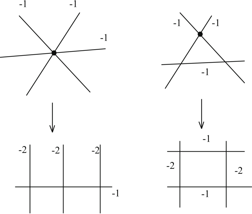
Suppose we have 3 negative curves that each intersect one another pairwise. Then, for example, we cannot distinguish the two cases depicted in Figure 4 given only the vector representations of the curves and their corresponding intersection matrix. In one case there are three (-1)-curves that all intersect at a single common point, and in the other case there are three distinct intersection points where each pair of curves intersect. But the blow up procedures for these two configurations are different. The case in which three negative curves intersect at a single point can in many situations be regarded as a special point in the moduli space of the surface (e.g. dP6) defined by Eff. In principle, this piece of information needs to be added along with the vector representation of the curves in Eff in order to fully specify the base, and this characterization of bases is finer than the notion that the surfaces are “of the same type”. In most situations in which configurations of this type occur, one can choose whether the case on the left or the case on the right in Figure 4 describes the geometry. In other cases of this type, however, it can occur that only one of the geometric possibilities can actually be realized. Distinguishing which of the possibilities is geometrically allowed seems in general to be a difficult problem. For the explicit classes of bases that we enumerate later in this paper, this kind of situation does not arise. But for a completely general analysis of bases giving elliptic Calabi-Yau threefolds with arbitrary Hodge numbers, a systematic methodology is needed for dealing with configurations with these kinds of issues. We give some simple examples here to illustrate the kinds of problems that can arise.
| curve | point | a | b | c | d | e | f | g | h | i |
|---|---|---|---|---|---|---|---|---|---|---|
| A | 1 | -1 | -1 | -1 | 0 | 0 | 0 | 0 | 0 | 0 |
| B | 1 | 0 | 0 | 0 | -1 | -1 | -1 | 0 | 0 | 0 |
| C | 1 | 0 | 0 | 0 | 0 | 0 | 0 | -1 | -1 | -1 |
| D | 1 | -1 | 0 | 0 | -1 | 0 | 0 | -1 | 0 | 0 |
| E | 1 | 0 | -1 | 0 | 0 | -1 | 0 | 0 | -1 | 0 |
| F | 1 | 0 | 0 | -1 | 0 | 0 | -1 | 0 | 0 | -1 |
| G | 1 | -1 | 0 | 0 | 0 | 0 | -1 | 0 | -1 | 0 |
| H | 1 | 0 | -1 | 0 | -1 | 0 | 0 | 0 | 0 | -1 |
| I | 1 | 0 | 0 | -1 | 0 | -1 | 0 | -1 | 0 | 0 |
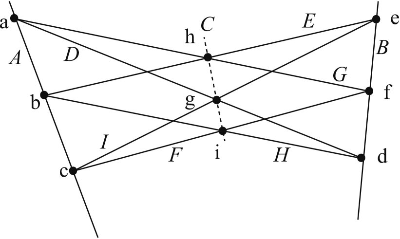
One particular situation of this type that can arise involves combinations of three negative curves that have to intersect at a single point. For example, consider the configuration of Sing, with , in Table 4; the corresponding geometrical picture is drawn in Figure 5. Note that in the last blow-up at point , lines , and are guaranteed to intersect at a single point, by Pappus’s theorem.
This phenomenon is a special case of the more general Cayley-Bacharach theorem (for a complete overview of this subject, see Eisenbud1996 ). Theorem CB4 in Eisenbud1996 says that if 2 curves and of degree and intersect at distinct points , and another curve of degree passes through points in , then passes through all points in .
The Charles theorem corresponds to the case , which in general states that if two cubic curves intersect at 9 points, then another cubic curve that passes through 8 of these 9 points must pass through the ninth point. Pappus’s theorem corresponds to the degenerate case where these three cubic curves are linear combinations of 3 lines respectively: , and as in Table 4. Note that the more general case of Charles’s theorem is operational in the construction of a rational elliptic surface, where after blowing up eight general points on , the ninth point blown up is the common point to a pencil (one-parameter family) of cubics that pass through the first eight points.
| curve | point | a | b | c | d | e | f | g | h |
|---|---|---|---|---|---|---|---|---|---|
| A | 1 | -1 | -1 | -1 | 0 | 0 | 0 | 0 | 0 |
| B | 1 | 0 | 0 | 0 | -1 | -1 | -1 | 0 | 0 |
| C | 1 | -1 | 0 | 0 | -1 | 0 | 0 | -1 | 0 |
| D | 1 | 0 | 0 | -1 | 0 | -1 | 0 | -1 | 0 |
| E | 1 | 0 | -1 | 0 | 0 | 0 | -1 | -1 | 0 |
| F | 1 | 0 | -1 | 0 | 0 | -1 | 0 | 0 | -1 |
| G | 1 | -1 | 0 | 0 | 0 | 0 | -1 | 0 | -1 |
| H | 1 | 0 | 0 | -1 | -1 | 0 | 0 | 0 | -1 |
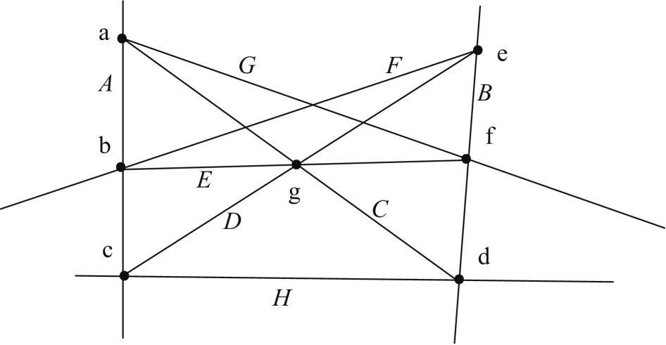
On the other hand, sometimes it is impossible for three negative curves to intersect at a single point. Consider the configuration with in Table 5. We draw the first 7 blow up points on a plane in Figure 6. We then blow up the point with the intersection properties described in Table 5. This requires that , and all intersect at a single point. From the combinatorics of the effective cone, it seems possible to blow up an eighth point to get curves with the intersection properties described in Table 5. In this situation, however, there is requirement that , and intersect at a single point, which is geometrically impossible. Hence the configuration in Table 5 is not allowed. Thus, the structure of the combinatorics of the effective cone is in general insufficient to guarantee that a set of three curves either can or cannot all intersect at a single point.
For a complete analysis of all bases, we would need a systematic way to distinguish between the following three possibilities in any given situation:
(1) Three negative curves must all intersect at a single point.
(2) Three negative curves cannot all intersect at a single point.
(3) Three negative curves may or may not intersect at a single point.
It seems possible that a systematic analysis using the generalized Caylay-Bacharach theorem can give a clear general answer in these situations, but we leave this to future studies.
One interesting aspect of these geometric issues is the question of how the allowed combinatorial structures for the effective cone can be understood from the point of view of the low-energy 6D supergravity theory. We return to this issue in the final section.
7 Finiteness of curves
Another difficulty that can arise in the complete classification of bases is the appearance of bases in which the cone of effective curves Eff has an infinite number of generators. In our classification program, in particular, the finite generation property of Eff is a prerequisite in Lemma 2. The finiteness of (-1)-curves on any given surface is, however, considered to be an open problem. A nice partial result in this direction is the theorem proved in Testa , which states that any surface with big anticanonical class has finitely generated Cox ring, which implies the finite generation of Eff and finiteness of (-1)-curves (for more information about Cox ring and finiteness see Ottem ). In the context of rational surfaces with effective anticanonical class, the phrase “big” in this context actually implies that one of the following conditions holds:
(1)
(2) , where and are two effective curves in Eff, and either or . Here the the two sets of indices satisfy , where “” means disjoint union.
(3) , where , and are three effective curves in Eff, and either or . Here the three sets of indices satisfy .
From the perspective of our recursive algorithm of finding all the (-1)-curves, these conditions can be understood in the following way:
If the condition (1) holds, then on average the entries in the -operation increase by after a -operation, which increases the degree of the curve by one. If one applies the -operation sufficiently many times, then the sum of the negative of any three entries will exceed , and then there is no -operation increasing the degree of curve. The sufficiency of the conditions (2) and (3) for guaranteeing a finitely generated effective cone can be argued in a similar way. For case (2) the way to perform a -operation while preserving the intersection number with and is to choose , . Then on average the entries () increase by , and the entries () increase by . Because , the set of -operations that increase the degree of the curve will not last forever. For case (3), the way to perform a -operation while preserving the intersection number with , and is to choose , , . On average the entries () increase by , the entries () increase by , and the entries () increase by . The possibility of having an arbitrarily high degree curve is also excluded by the condition .
Although most bases that we are interested in for F-theory constructions have finitely generated effective cones, one can also construct surfaces with an infinite number of (-1)-curves, which may nonetheless be good bases for F-theory compactification. For example, we mention above the case of a rational elliptic surface. An explicit example is an base with
| (35) | |||||
This is a generalized del Pezzo surface with three -2 curves. This surface clearly satisfies the condition that is in the effective cone, but also admits an infinite number of -curves on the boundary of the effective cone. We can prove this as follows: suppose we pick an exceptional curve . Then at step 1 we perform the -operation with entries . At step 2 we perform the -operation with entries . At step 3 we perform -operation with entries , and we infinitely repeat these three steps. The intersection product with the three curves in Sing is invariant during this process. The degree of the curve at step can be explicitly computed, and is equal to . This means that the process will give arbitrarily high degree curves, hence the number of (-1)-curves is infinite.
Bases with an infinite number of generators for the effective cone are difficult to incorporate into the kind of analysis we are doing here. We cannot compute the dual cone of Neg, nor study the blow up of the surface in an efficient way. It would be possible in practice to avoid this problem by stopping when the number of curves produced by the algorithm exceeds a certain number, assuming that in this case the surface contains an infinite number of (-1)-curves, and the branch can be discarded. It seems based on some limited evidence that the only situations where an infinite number of negative self-intersection curves arise is on a relatively small number of limiting bases that cannot be further blown up, and which are associated with Calabi-Yau threefolds having quite small . And it is not clear whether bases with this infinite number of generators really give acceptable F-theory models. We leave a further exploration of these questions, however, to future work.
8 The algorithm
In this section we give a finite recursive algorithm for generating general bases, with specific prescriptions for dealing with the various potential complications discussed in preceding sections.
(1) We start from a base , with Picard rank and a vector representation of negative curves Neg, Sing Neg. This data should always be finite.
(2) We construct all blowups of in three possible ways: blow up the intersection point of two curves Neg, blow up a generic point on a curve Neg, or blow up a generic point on the plane. We do not consider blowups at points at which three or more negative curves intersect. The special blow-ups are also excluded in the current algorithm.
After this step we have the new Sing.
(3) With this new Sing, we use the -process to generate the (-1)-curves on . In practice, we just start from all the curves of degree 0 and degree 1. If the number of curves in this step reaches a certain large value (such as 500 or 1,000), then the number of generators is considered to be infinite and the base is discarded. This situation turns out not to occur in the regimes of this paper.
(4) Then we need to check if the degrees of vanishing of are greater or equal than on any of the divisors (see Table 1). If this happens then this singularity cannot be resolved and the base is discarded.
Practically, we use the method of Zariski decomposition, as in Classbasis . The actual algorithm is, we decompose to
| (36) |
The integral coefficients indicate the orders of vanishing of on the divisors . And are all the elements in Neg. The residual part should be an effective -divisor, which intersects non-negatively with all curves . We start from , and examine for every . If this quantity is negative for , then we add a minimal value to that will make this quantity non-negative and do the check again, until for every . If in the process any reaches a certain value (11 for ), then the singularity is too bad to be resolved. When this happens the process stops and the base is discarded.
If there is set of coefficients that pass the check, then we examine all the intersection points of pairs of negative curves and . If the sum of coefficients for , then this intersection point needs to be blown up.
Furthermore, bases containing (-9),(-10),(-11)-curves are not good, since there are always points on these curves. Such points need to be blown up until the curve of large negative self-intersection becomes a (-12)-curve. (Note that the points blown up in this process could be generic points on these curves or points where they intersect with other negative curves). The base is good only when no more points of this kind need to be blown up.
Applying this method, one can derive the restrictions on curves and intersecting curve configurations to give all the connected subgraphs that can appear without any (-1)-curves. These are just the NHCs listed in Table 2, along with configurations with only (-2)-curves. The latter case corresponds to Dynkin diagrams of Lie algebras and affine Lie algebras. There are additional restrictions on the ways in which different NHCs can consistently connect to one other. The NHC linking rules listed in Classbasis , augmented by a further set of branching conditions on curves of self-intersection below in semi-toric , give a complete set of such rules. In our analysis here, these rules automatically are enforced by the conditions that there are no curves or points in the base.
(5) If no additional points need to be blown up, then we compute the generators of the dual cone of Neg. This is known to be a hard problem, the exact algorithm is described in (Fulton, , p. 11). If the vectors in Neg are dimensional, then one computes the normal vector to each of the -dimensional facets. Then if or intersects non-negatively with all , then or is a generator of Nef. Hence if Neg, then the computational complexity is at least . This turns out to be the major computational difficulty in this program.
After all the generators of the dual cone of Neg are found, we check if all the generators are non-negative. If not, we add the negative ones into Neg. We repeat the step (4)(5), and finally the dual cone of Neg will be free of negative generators, which means that the set Neg contains the complete set of (-1)-curves.
We then further check if intersects non-negatively with all the generators. If not, then is not in the effective cone hence the base is not allowed.
(6) If the previous test is passed, then this base is good. The next step is checking if the intersection structure is isomorphic to one of the bases generated before. The graph isomorphism problem is also known to be hard; it is not clear if there exists a polynomial algorithm. In practice we used the “VFlib” library developed by Pasquale Foggia vflib .
(7) If all the tests are passed, add this base to solution set and restart step (1) using .
The overall starting points are the bases with that come from blowing up , and which have no (-9),(-10),(-11) curves. We list their Neg below (the l.h.s. is the cyclic toric diagram for these bases ):
| (37) |
So and are not counted in the solution set and they have to added in by hand.
Using this algorithm can produce a finite list of possible bases in a specific desired range. The possible sources of incompleteness or inaccuracy in such a list are as follows:
(i) Bases where the effective cone has an infinite number of generators, or a very large number that exceeds the arbitrary cutoff in the code, will be missed.
(ii) Bases that are produced by “special blowups” giving curves of self-intersection -2 or below, or by blowing up points at the intersection of more than two negative curves, will be missed by this algorithm.
(iii) If there are bases in which, as in Pappus’s theorem, a certain combination of more than two negative self-intersection curves are forced to intersect at a common point, this algorithm may generate spurious bases that appear to have an acceptable combinatorial structure for the cone of effective curves, but which do not correspond to actual surfaces.
In the following sections we present some classification results of bases under certain limits. We have checked that in these regimes none of the subtleties just mentioned occurs, so we indeed generate all the possible bases in these regimes.
9 Classification of all bases with rk(Pic
The first subset that we enumerate explicitly is the set of bases with rk(Pic. We wish to explicitly determine the set of all combinatorially distinct effective cones that are possible for bases in this range; this determines all topological types of bases, for each of which we can compute Hodge numbers for the generic elliptic fibration over that base. For this set of bases, none of the problematic issues are relevant. The smallest value of rk(Pic where the issue arises that three negative curves may intersect each other is 7, where we can have , , . Hence this subtlety will not affect the classification of types of bases with rk(Pic. Note, however, that at rk(Pic, a situation arises already where there are non-isomorphic surfaces of the same type. On , we can blow up six points in such a way that we can realize either of the two configurations in Figure 4. These surfaces are treated identically in our combinatorial analysis. Blowing up these non-isomorphic surfaces gives topologically different surfaces with rk(Pic, so a systematic way of treating this issue would be necessary to continue this analysis to higher values of . Within this range of consideration, the problem of special blow-ups also is not a problem, since the shortest vector representation of a curve that comes from a special blow-up is . And the number of generators of the effective cone is finite for all surfaces in this range. Thus, the list of all bases with rk(Pic generated by our algorithm is indeed complete.
In total there are 468 bases with rk(Pic. This includes the surfaces and with or 12. Among these, 245 are non-toric and 177 are not included in the semi-toric list in semi-toric . All previously identified toric and semi-toric bases appear in the set generated by our algorithm, which gives a check on the correctness and completeness of the result. 111Note that for the purposes of counting and comparison in this paper we include among toric and semi-toric bases those bases that have toric or semi-toric structure including curves of self-intersection ; in some cases such bases are not really toric or semi-toric once the (4, 6) singularities on the etc. curves are blown up. We include these bases however in the toric and semi-toric sets since they can be generated effectively using the corresponding toric or semi-toric approach. This technical distinction is discussed further in semi-toric . A detailed breakdown of the number of bases with each value of Picard rank that fit in each category is given in Figure 7.
At low values of , the set of bases generated can be understood directly along the lines of the discussion in Section 3 and Figure 3. For the only bases are and the Hirzebruch surfaces. The blowups to give a set of 9 toric surfaces with toric divisors having self-intersection with . There are 22 surfaces at , of which three are non-toric. The three non-toric bases are those resulting from blowing up the middle curve in the chain of curves at a generic point, when . (For or below, this construction gives intersecting curves with , which gives rise to a singularity at the intersection point.) The non-toric example in Figure 3 is the example of this type with . Continuing further, at there are a total of 49 distinct base topologies, of which 27 are toric, another 7 are semi-toric but not toric, and another 15 are non-toric and cannot be identified by toric or semi-toric analysis. As increases, the fraction of bases that are non-toric increases.
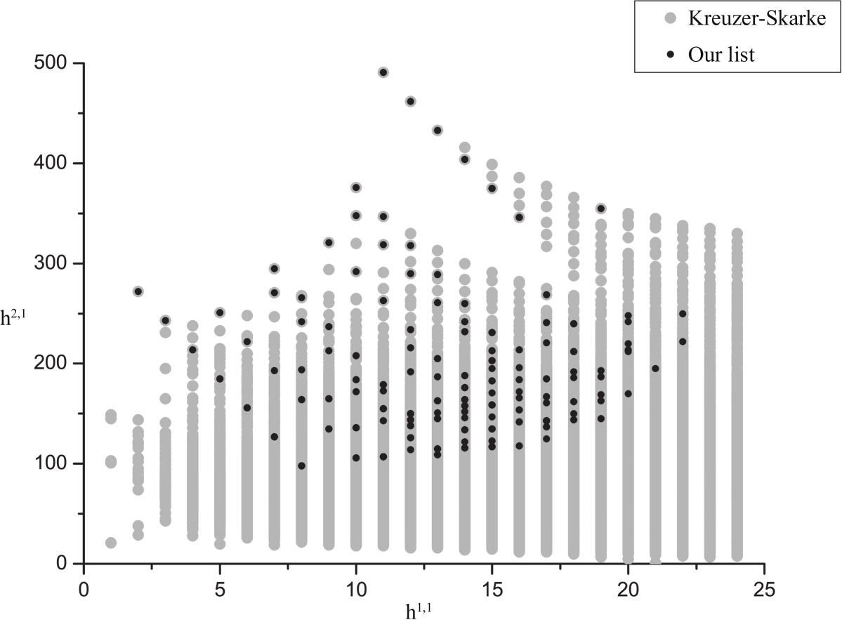
We plot the Hodge numbers of the generic elliptically fibered Calabi-Yau threefolds over the bases in this set in Figure 8. We also plot the Hodge numbers in the Kreuzer-Skarke database Kreuzer-Skarke . In principle, any elliptically fibered Calabi-Yau threefold with should be supported over one of the bases in this class. Note that many of the Hodge number pairs in this range can be realized by tuning Weierstrass models over the bases we have identified to realize larger gauge groups associated with enhanced Kodaira singularities, along the lines of the analysis in JohnsonTaylor . For example, the Kreuzer-Skarke list contains a Calabi-Yau threefold with Hodge numbers . This Calabi-Yau can be realized by tuning an gauge group on the divisor class in . Similarly, the Calabi-Yau with Hodge numbers can be realized by tuning an on a quadratic curve in the divisor class in , etc. Note, however, that this analysis guarantees that the Calabi-Yau’s with certain large Hodge numbers such as cannot be realized as elliptic fibrations.
The list also contains all the generalized del Pezzo surfaces listed in Derenthal from degree 6 to degree 3. The algorithm presented in this paper is a potential tool to generate all the generalized del Pezzo surfaces. The number of (-1)-curves on generalized del Pezzo surfaces are listed in Derenthal . These numbers exactly agree with the numbers generated with our method in Proposition 1. For instance, consider , if Sing or , then the number of -curves is exactly 21, which can be found in Table 7 of Derenthal . We can also run this algorithm for generalized del Pezzo surfaces up to , restricting to bases without curves or below. For when the case where three curves all meet at a point is ignored, we get 46 different intersection structures, matching the results of Derenthal . When one allows three curves to meet at a point, a new base with 7 (-2)-curves that do not intersect each other appears. This base is labelled by in the literature, and it only occurs over a field of characteristic 2. From our point of view, this base is forbidden by a geometric obstruction that is not apparent from the combinatorics of the effective cone. The complete list of all 47 bases including the base is given in Urabe . Similarly, for , the algorithm when triple intersections (but not special blow-ups) are allowed produces 76 bases, including the 74 identified in Derenthal and two others that appear in Urabe that have geometric obstructions over . The list in Urabe also contains one further base with , which is not identified by our algorithm and also has a geometric obstruction over .
When applied to bases with rk(Pic, we might hope to use this approach to reproduce the complete list of types of rational elliptic surfaces with degenerate elliptic fibers as divisors, i.e., Persson’s list Persson Miranda . This would provide a simple context in which to attempt to systematically address the issues of multiply intersecting curves, special blowups, and potentially infinite numbers of generators for the effective cone.
10 Classification of all bases for elliptic Calabi-Yau threefolds with
Another set of bases that we can completely classify is the set of bases that support elliptic Calabi-Yau threefolds with . This subset is relatively easy to study, because it turns out that the difference between and rk(Pic is small. Hence the dual cone problem is easier to solve, though still computationally expensive. Also, the situations in which three negative curves intersect each other or the dual of Neg contains a negative curve never happen, nor does an infinite number of negative curves ever arise. The only issue that could in principle make our list incomplete is the presence of special blow-ups. Recall that special blow-ups only happen when contains a curve with self-intersection or lower, and the last entry in its vector representation is (-2) or lower. We begin by discussing the results of our analysis, and then in subsection 10.3 we explain why special blow-ups can essentially be ruled out for this class of bases. The analysis described in §10.3 also makes it clear that in the range we do not expect higher degree curves, so that it should not be necessary to check the dual cone. We nonetheless explicitly checked the dual cone in the cases where and confirmed that in this range the effective cone is automatically produced correctly by -operations on low-degree curves, and does not miss any higher degree curves. We did not explicitly check this in the range , due to the computational time needed, but we expect from the arguments in §10.3 that the results in that range would be the same as those for .
10.1 Statistics of bases giving generic EFS CY3’s with large
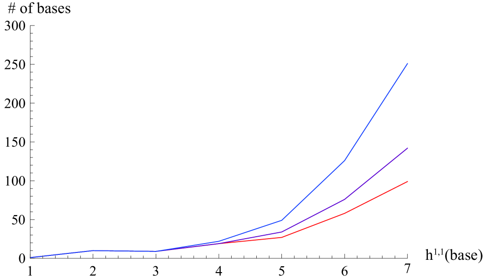
In total our algorithm produces 6511 bases over which the generic elliptic Calabi-Yau threefold has . This set of bases includes and , with or 12. All the 3871 toric and toric + semi-toric bases identified in Toric ; semi-toric giving threefolds with can be found in our list (including ones generated from blowing up -9/-10/-11 curves at generic points). Hence the number of new bases which is not in the list of semi-toric is 2640.
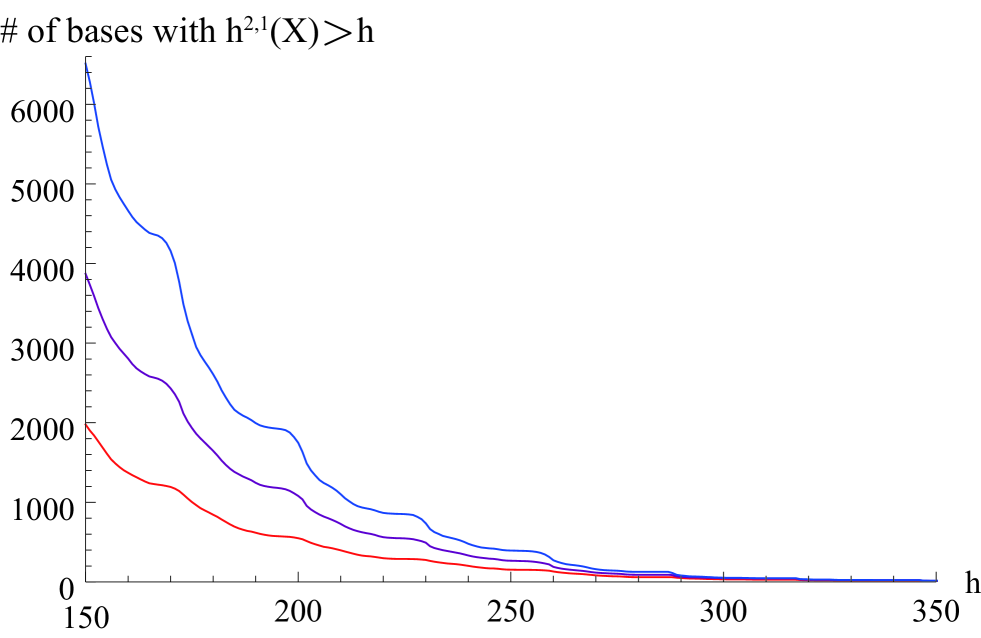
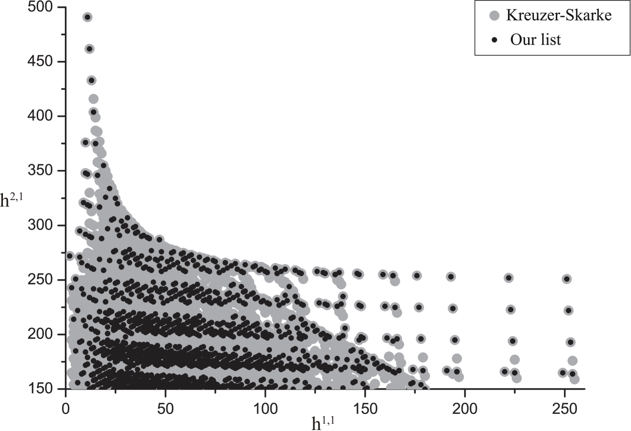
We plot the Hodge numbers of the generic elliptic Calabi-Yau threefolds over this set of bases in Figure 10. Generic elliptic fibrations over the 6511 distinct bases give CY threefolds with 1278 distinct Hodge number pairs. For very large , as discussed in JohnsonTaylor , all known Calabi-Yau threefolds can be realized as elliptic fibrations over toric or semi-toric bases. The first non-toric base arises from a Calabi-Yau with Hodge numbers ; these Hodge numbers can also, however, be found from a Calabi-Yau that is elliptically fibered over a toric base, where the toric base is a limit of the non-toric base containing an extra curve. Similar situations arise at other large values of . The largest value of at which there is a non-toric base with no toric equivalent is at the Hodge numbers . In the following subsection we describe this base, as well as other new non-toric bases that we have identified with generic elliptic fibrations having Hodge numbers that are not in the Kreuzer Skarke database.
A graph of the number of toric, semi-toric, and non-toric (meaning neither toric nor semi-toric) bases with Hodge numbers exceeding particular values of is shown in Figure 9. It is notable that the number of non-toric constructions is not dramatically larger than the number of toric bases anywhere in the range considered. In principle, one might have imagined that toric constructions would only represent a very specialized class of Calabi-Yau threefolds. At least for elliptic CY threefolds with , we see that this is not the case. In fact, toric geometry seems to be surprisingly effective at constructing a representative sample of Calabi-Yau threefolds at large Hodge numbers.
10.2 New Calabi-Yau threefolds
We have identified 15 bases that give rise to elliptic Calabi-Yau threefolds with Hodge numbers that are not in the Kreuzer-Skarke database. Their Hodge numbers are:
| (38) |
The mirrors of these Calabi-Yau threefolds also do not appear in the Kreuzer-Skarke database, so this represents 30 new Calabi-Yau threefolds. The fact that only 15 of the 1278 Hodge number pairs produced by our algorithm represent Calabi-Yau threefolds with Hodge numbers that are not produced through toric constructions suggests that toric methods are remarkably effective in producing a representative sample of Calabi-Yau manifolds, at least for elliptic threefolds with large Hodge numbers. Note that while 8 semi-toric bases were identified in semi-toric that give rise to elliptic Calabi-Yau threefolds with Hodge numbers not included in the Kreuzer-Skarke database, the largest Hodge number for any of these was .
The new Calabi-Yau threefold with the largest value of , which has Hodge numbers , can be understood by explicitly analyzing the base geometry. This geometry is closely related to the set of bases studied in JohnsonTaylor . If we begin with the toric base having self-intersections
| (39) |
which is associated with a Calabi-Yau having Hodge numbers , and then blow up a generic point on the curve, we get a non-toric base having no toric equivalent, over which the generic Calabi-Yau elliptic fibration has Hodge numbers . The shift by in arises from a shift of from the blowup, and from the difference in the contribution to from the dimensions of the groups . By explicitly analyzing possible sequences of blowups on a single fiber, it can be shown fairly readily that this base is the first one encountered as decreases that is non-toric and is not equivalent to a toric base. Note that after the non-toric blowup it is not possible to blow up another point on the new curve, since the non-Higgsable cluster cannot be adjacent to a cluster Classbasis . One can blow up the point between the and curves, giving a new base with generic elliptic Calabi-Yau having Hodge numbers . This non-toric base is not equivalent to a toric base, but has the same Hodge numbers as a closely related toric base. Blowing up a generic point on the base gives a base with Hodge numbers , also on the list above. And the base with Hodge numbers can be constructed by starting with a toric base having self-intersections and blowing up a point on the middle curve in the last sequence. The rest of the new bases and associated Calabi-Yau threefolds can be understood in a similar fashion.
Note that all of these non-toric constructions are fairly close to toric bases, consisting for the most part of long linear chains of non-Higgsable clusters connected by curves, with occasional adornments that take the bases outside the toric class. While we expect that at smaller the intersection structure of non-toric bases becomes more complex, the general picture that we see at large matches well with the results of semi-toric , and suggest that going beyond toric bases, and including branching and loops in the intersection structure of the base does not dramatically increase the complexity or number of possible base surfaces that can support elliptic Calabi-Yau threefolds.
10.3 Special blow-ups
We conclude this section with a brief description of why special blow-ups do not occur in this set of bases associated with elliptic Calabi-Yau’s having large . While we do not have a formal mathematical proof that this cannot occur, we argue below that special blowups cannot arise for any base giving a generic elliptic fibration with . Related arguments explain why at large there are no issues with multiple intersecting negative curves, or infinitely generated effective cones.
In the full set of data that we generated without including the possibility of special blow-ups, it turns out that there is never a negative curve with a (-2) in the vector representation; in fact there is not even a single negative curve with degree 2 or higher in any of the bases. The reason is essentially that curves of high degree are strongly constrained in the presence of non-Higgsable clusters. For instance, when we consider the bases that come from blowing up , the (-12)-curve tightly restricts the possible form of negative curves. To ensure that a negative curve intersects non-negatively with the (-12)-curve, all the curves with degree 2-5 are excluded, and the first valid example of higher degree is . In our data it turns out that there is never a (-1)-curve in this form. This is due to the fact that we only keep bases with large . The same features that obstruct the appearance of such a (-1)-curve even more strongly obstruct the appearance of a (-2)-curve or below that could arise from a special blowup..
To be more explicit, let us attempt to identify the base with maximal that arises as a blowup of , and which contains the (-1)-curve . This is the first -curve of higher degree that can appear on a blowup of . We claim that the base of interest is just blown up at 13 generic points, denoted by Bl, with . This base has no NHC aside from the original (-12) curve. It is not possible to keep the same degree 6 (-1) curve and increase by choosing specific points to generate additional nonabelian groups, since, for example, a (-3) curve that could support an factor would need to be on a curve of the form e.g. , which cannot happen as it would have negative intersection with the degree 6 negative curve. Further non-Abelian non-Higgsable gauge groups can be added by further blowups, but this procedure will always lower . One may wonder if there is a base that contains a (-1)-curve like with greater than 114. This is impossible, because one can permute the last (-1)-entry with this 0-entry in the middle. For other curves on , this permutation is always feasible except for the curve of the form , where the 1-entry is going to be permuted. However this curve is not compatible with , because the intersection number between them is negative. After the permutation, the base becomes a blow up of Bl, hence its is smaller than 114. This shows that a degree 6 curve of self-intersection -1 cannot arise from blowups of for any base associated with an elliptic Calabi-Yau having .
Now considering other type of curves with degree higher than 1 on blowups of , the base with maximal that contains the curve is also the base with smallest Picard rank (or length of vector representation). For example, the curve
| (40) |
is a curve that can be generated by special blow-up. The maximal NHC that is compatible with this are three (-3)-curves of the form . Hence the maximal . In general the maximal of bases containing these types of curves which are generated by special blow-up is even less than 114, hence in our regime they will never appear. This conclusion seems quite clear from the form of curves of degree , though we have not attempted a systematic and complete mathematical analysis of all possibilities.
Similarly for the bases that come from blowing up , which contains a (-8)-curve , the lowest degree negative curve with degree greater than 1 is . The maximal . We list these numbers for each in Table 6; the largest value in that table is for . The conclusion is that special blow-ups should not bother us in the regime .
| 0,1,2 | 3 | 4 | 5 | 6 | 7 | 8 | 12 | |
|---|---|---|---|---|---|---|---|---|
| max | 127 | 135 | 126 | 121 | 118 | 116 | 115 | 114 |
The absence of negative curves of degree higher than one helps to explain why there are no problems with configurations of multiple mutually intersecting curves, or infinitely generated effective cones, when is reasonably large. For example, for bases that arise as blowups of , and on which the only curves are of degree 1, such curves always take the form or . It is easy to see that there cannot be three curves in these forms that all intersect pairwise. Furthermore, there are clearly a finite number of negative curves on any such base. While the constraints are weaker for bases that arise as blowups of for small , the only surfaces without curves of self-intersection -3 or below are the generalized del Pezzo surfaces, and we know that the first appearance of three mutual intersecting curves in that context occurs on , associated with a Calabi-Yau having .
Thus, it seems in principle that it should be possible to carry out the systematic analysis of bases as far down as roughly before any of these issues will arise. For bases without higher-degree negative curves, the algorithm can also be made more efficient since it is not necessary to check the dual cone condition. The remaining issue which this does not address, however, is whether is in the effective cone for all such bases.
11 Conclusions
In this paper we have developed a combinatorial approach to exploring the set of smooth non-toric base surfaces that can support elliptically fibered Calabi-Yau threefolds. This approach has enabled us to carry out a systematic enumeration of base surfaces with small Picard number and base surfaces that support elliptic Calabi-Yau manifolds with large Hodge number .
There are a few issues that make it difficult to extend the enumeration carried out here to the complete set of non-toric bases associated with arbitrarily small values of . In particular, the combinatorial data of the cone of effective divisors in that we use here to characterize surfaces does not capture all geometric information; in some cases there are surfaces “of the same type” that share this combinatorial description but have different more detailed structure. Related to this, in some cases there are “special blow-ups” that produce curves of self-intersection -2 or below that are difficult to systematically detect. Neither of these issues arises in the specific classes of surfaces that we have constructed here, but they would need to be dealt with for a complete enumeration of bases, or of elliptic Calabi-Yau threefolds. There is also the issue that the number of generators of the effective cone can be infinite; this seems to only occur, however, at limiting bases that cannot be blown up further to give further valid bases for elliptic CY fibrations.
One of the main lessons of this work is that including completely general non-toric bases does not seem to dramatically expand the range of possible constructions for elliptic Calabi-Yau threefolds, at least at large Hodge number. This extends further the qualitative results of semi-toric , which showed that adding nontrivial branching and loops to the intersection structure of negative self-intersection curves in the base does not dramatically increase complexity. Indeed, particularly at large Hodge numbers it seems that toric bases do a remarkably good job of characterizing the set of possible bases for elliptic Calabi-Yau threefolds, at least at a qualitative level, and that while adding bases with semi-toric or non-toric structure increases the number of possibilities, it does not do so by many orders of magnitude.
The bases constructed here could be used in principle to construct all possible elliptic Calabi-Yau threefolds with , by including all tunings of additional nonabelian gauge groups, matter representations at codimension two, and abelian gauge groups, along the lines of JohnsonTaylor . While this would be a computationally intensive endeavor, and there are still some open questions regarding possible matter representations and codimension two singularities, much of the understanding is in place to make this a tractable proposition. Recent work from a number of different directions WT-Hodge ; Candelas-c-Skarke ; JohnsonTaylor ; Gray-hl suggests that the majority of known Calabi-Yau threefolds are elliptic, particularly those with large Hodge numbers. It is interesting to speculate that the set of elliptic CY threefolds that could be constructed using the bases determined here could in fact comprise all, or almost all, of the Calabi-Yau manifolds with , independent of the elliptically fibered condition. Of course, more insight into the structure of general Calabi-Yau threefolds would be necessary to verify any such claim.
Some of the issues encountered in this paper pose interesting questions for the program of “string universality” in six dimensions. It is known that all quantum-consistent massless spectra for 10-dimensional theories of gravity with minimal supersymmetry are realized in string theory 10D-universality , and it has been conjectured that a similar statement is true in six dimensions 6D-universality . The close connection between the geometry of F-theory constructions and the structure of the corresponding low-energy six-dimensional supergravity theory was used in KMT ; KMT-II to relate constraints between these two pictures. In particular, the intersection structure on the F-theory base maps to and constrains the structure of the dyonic string lattice in the 6D theory Seiberg-Taylor . From this point of view, the set of F-theory vacua on Calabi-Yau manifolds with large , corresponding in the 6D supergravity picture to theories with large numbers of neutral scalar fields, may be a natural context in which to strengthen the evidence for string universality in 6D. For example, it would be interesting to try to demonstrate that the only consistent low-energy 6D supergravity theories with one supersymmetry and more than 150 neutral scalar fields are those that arise from F-theory constructions on the bases we have constructed here. One interesting challenge for extrapolating such a program to lower is to find a low energy understanding of the different types of constraints discussed in §6 associated with e.g. Pappus’s theorem, or the configuration described in Table 5, each of which indicates that a certain structure of effective cone for the 6D supersymmetric string charge lattice that may appear consistent, cannot be realized in F-theory by a sensible base geometry. Such issues may provide a useful insight into the precise correspondence between UV consistency conditions on low-energy six-dimensional supergravity theories and the geometry of F-theory constructions.
The datasets described in Sections 9 and 10 are available online at online-data .
Acknowledgements
We would like to thank Lara Anderson, James Gray, Sam Johnson, Gabriella Martini, and David Morrison for helpful discussions. This research was supported by the DOE under contract #DE-SC00012567.
References
- (1) K. Matsuki, “Introduction to the Mori Program,” Springer-Verlag, Berlin (2002).
- (2) P. Candelas, G. T. Horowitz, A. Strominger and E. Witten, “Vacuum Configurations for Superstrings,” Nucl. Phys. B 258, 46 (1985).
- (3) P. Candelas, A. M. Dale, C. A. Lutken and R. Schimmrigk, “Complete Intersection Calabi-Yau Manifolds,” Nucl. Phys. B 298, 493 (1988).
- (4) V. Batyrev, “Variations of the mixed Hodge structure of affine hypersurfaces in algebraic tori,” Duke Math. Journ. 69, 349 (1993).
- (5) M. Kreuzer and H. Skarke, “Complete classification of reflexive polyhedra in four-dimensions,” Adv. Theor. Math. Phys. 4, 1209 (2002), arXiv:hep-th/0002240; data available online at http://hep.itp.tuwien.ac.at/ kreuzer/CY/
- (6) R. Altman, J. Gray, Y. H. He, V. Jejjala and B. D. Nelson, “A Calabi-Yau Database: Threefolds Constructed from the Kreuzer-Skarke List,” JHEP 1502, 158 (2015) arXiv:1411.1418 [hep-th].
- (7) B. Jurke, “Calabi-Yau 3-fold explorer,” available online at benjaminjurke.net/show/calabi-yau-manifolds
- (8) R. Davies, “The Expanding Zoo of Calabi-Yau Threefolds,” Adv. High Energy Phys. 2011, 901898 (2011), arXiv:1103.3156 [hep-th].
- (9) Y. H. He, “Calabi-Yau Geometries: Algorithms, Databases, and Physics,” Int. J. Mod. Phys. A 28, 1330032 (2013), arXiv:1308.0186 [hep-th].
- (10) M. Gross, “A finiteness theorem for elliptic Calabi–Yau threefolds,” Duke Math. Jour. 74, 271 (1994).
- (11) C. Vafa, “Evidence for F-Theory,” Nucl. Phys. B 469, 403 (1996), arXiv:hep-th/9602022.
- (12) D. R. Morrison and C. Vafa, “Compactifications of F-Theory on Calabi–Yau Threefolds – I,” Nucl. Phys. B 473, 74 (1996) arXiv:hep-th/9602114;
- (13) D. R. Morrison and C. Vafa, “Compactifications of F-Theory on Calabi–Yau Threefolds – II,” Nucl. Phys. B 476, 437 (1996) arXiv:hep-th/9603161.
- (14) D. R. Morrison and W. Taylor. “Classifying bases for 6D F-theory models.” Central European Journal of Physics 10.5 (2012): 1072-1088, arXiv:1201.1943 [hep-th].
- (15) D. R. Morrison and W. Taylor. “Toric bases for 6D F-theory models.” Fortschritte der Physik 60.11-12 (2012): 1187-1216, arXiv:1204.0283 [hep-th].
- (16) G. Martini and W. Taylor. “6D F-theory models and elliptically fibered Calabi-Yau threefolds over semi-toric base surfaces.” arXiv:1404.6300 [hep-th].
- (17) S. B. Johnson and W. Taylor. “Calabi-Yau threefolds with large ,” arXiv:1406.5214 [hep-th].
- (18) J. J. Heckman, D. R. Morrison and C. Vafa, “On the Classification of 6D SCFTs and Generalized ADE Orbifolds,” JHEP 1405, 028 (2014) arXiv:1312.5746 [hep-th].
- (19) M. Del Zotto, J. J. Heckman, D. R. Morrison and D. S. Park, “6D SCFTs and Gravity,” arXiv:1412.6526 [hep-th].
- (20) J. J. Heckman, D. R. Morrison, T. Rudelius and C. Vafa, “Atomic Classification of 6D SCFTs,” arXiv:1502.05405 [hep-th].
- (21) W. P. Barth, K. Hulek, C. A. M. Peters, A. Van de Ven, “Compact complex surfaces,” Springer, 2004.
- (22) A. Grassi, “On minimal models of elliptic threefolds,” Math. Ann. 290 (1991) 287-301.
- (23) D. R. Morrison, “TASI lectures on compactification and duality,” hep-th/0411120.
- (24) F. Denef, “Les Houches Lectures on Constructing String Vacua,” arXiv:0803.1194 [hep-th].
- (25) W. Taylor, “TASI Lectures on Supergravity and String Vacua in Various Dimensions,” arXiv:1104.2051 [hep-th].
- (26) N. Nakayama, “On Weierstrass models”, in Algebraic geometry and commutative algebra, Vol. II, Kinokuniya, Tokyo, 1988, pp. 405-431.
- (27) K. Kodaira, “On compact analytic surfaces. II, III”, Ann. of Math. (2) 77 (1963) 563-626, 78 (1963) 1-40.
- (28) J. Tate, “Algorithm for determining the type of a singular fiber in an elliptic pencil, Modular functions of one variable, IV” (Proc. Internat. Summer School, Univ. Antwerp, Antwerp, 1972), Lecture Notes in Math., vol. 476, Springer, Berlin, 1975, pp. 33-52.
- (29) M. Bershadsky, K. A. Intriligator, S. Kachru, D. R. Morrison, V. Sadov and C. Vafa, “Geometric singularities and enhanced gauge symmetries,” Nucl. Phys. B 481, 215 (1996) arXiv:hep-th/9605200.
- (30) S. Katz, D. R. Morrison, S. Schafer-Nameki and J. Sully, “Tate’s algorithm and F-theory,” JHEP 1108, 094 (2011) arXiv:1106.3854 [hep-th].
- (31) A. Grassi and D. R. Morrison, “Anomalies and the Euler characteristic of elliptic Calabi-Yau threefolds,” arXiv:1109.0042 [hep-th].
- (32) W. Taylor, “On the Hodge structure of elliptically fibered Calabi-Yau threefolds,” JHEP 1208, 032 (2012) arXiv:1205.0952 [hep-th].
- (33) D. R. Morrison, D. Park, and W. Taylor, to appear.
- (34) C. Schoen, “On fiber products of rational elliptic surfaces with section,” Math. Z., 197, 177-199 (1988).
- (35) E. Looijenga. “Rational surfaces with an anti-canonical cycle.” Annals of Mathematics (1981): 267-322.
- (36) B. Harbourne. “Anticanonical rational surfaces.” Transactions of the American Mathematical Society 349.3 (1997): 1191-1208, arXiv:alg-geom/9509001.
- (37) P. Griffiths and J. Harris. Principles of algebraic geometry. Vol. 52. John Wiley & Sons, 2011.
- (38) J. Kollár. Rational curves on algebraic varieties. Vol. 32. Springer, 1996.
- (39) L. Caporaso and J. Harris. “Enumerating rational curves: the rational fibration method.” Compositio Mathematica 113.02 (1998): 209-237, arXiv:alg-geom/9608023.
- (40) L. Caporaso and J. Harris. “Parameter spaces for curves on surfaces and enumeration of rational curves.” Compositio Mathematica 113.02 (1998): 155-208 arXiv:alg-geom/9608024.
- (41) M. Artebani and A. Laface, “Cox rings of surfaces and the anticanonical Iitaka dimension,” Advances in Mathematics 226.6 (2011): 5252-5267, arXiv:0909.1835 [math.AG].
- (42) U. Derenthal. “Singular Del Pezzo surfaces whose universal torsors are hypersurfaces.” Proceedings of the London Mathematical Society 108.3 (2014): 638-681, arXiv:math/0604194.
- (43) U. Derenthal. Geometry of universal torsors, dissertation, Universität Göttingen. http://resolver.sub.uni-goettingen.de/purl/?webdoc-1331.
- (44) M. Nagata. “On rational surfaces, II.” Memoirs of the College of Science, University of Kyoto. Series A: Mathematics 33.2 (1960): 271-293.
- (45) Yu I. Manin. Cubic forms: algebra, geometry, arithmetic. Elsevier, 1986.
- (46) D. Eisenbud, M. Green, and J. Harris. “Cayley-Bacharach theorems and conjectures.” Bulletin of the American Mathematical Society 33.3 (1996): 295-324.
- (47) D. Testa, A. Várilly-Alvarado, and M. Velasco. “Big rational surfaces.” Mathematische Annalen 351.1 (2011): 95-107, arXiv:0901.1094 [math.AG].
- (48) J. C. Ottem. “Cox rings of projective varieties.”, dissertation, University of Oslo (2009).
- (49) W. Fulton. Introduction to toric varieties. No. 131. Princeton University Press, 1993.
- (50) The VFLib Graph Matching Library, version 2.0 by Pasquale Foggia.
- (51) T. Urabe, “On singularities on degenerate del Pezzo surfaces of degree 1, 2,” Proc. Symp. Pure Math. 40, part 2, 587 (1983).
- (52) U. Persson. “Configurations of Kodaira fibers on rational elliptic surfaces.” Mathematische Zeitschrift 205.1 (1990): 1-47.
- (53) R. Miranda. “Persson’s list of singular fibers for a rational elliptic surface.” Mathematische Zeitschrift 205.1 (1990): 191-211.
- (54) P. Candelas, A. Constantin and H. Skarke, “An Abundance of K3 Fibrations from Polyhedra with Interchangeable Parts,” Commun. Math. Phys. 324, 937 (2013) arXiv:1207.4792 [hep-th].
- (55) J. Gray, A. S. Haupt and A. Lukas, “Topological Invariants and Fibration Structure of Complete Intersection Calabi-Yau Four-Folds,” JHEP 1409, 093 (2014) arXiv:1405.2073 [hep-th].
- (56) A. Adams, O. DeWolfe and W. Taylor, “String universality in ten dimensions,” Phys. Rev. Lett. 105, 071601 (2010) arXiv:1006.1352 [hep-th].
- (57) V. Kumar and W. Taylor, “String Universality in Six Dimensions,” arXiv:0906.0987 [hep-th].
- (58) V. Kumar, D. R. Morrison and W. Taylor, “Mapping 6D supergravities to F-theory,” JHEP 1002, 099 (2010) arXiv:0911.3393 [hep-th].
- (59) V. Kumar, D. R. Morrison and W. Taylor, “Global aspects of the space of 6D supergravities,” JHEP 1011, 118 (2010) arXiv:1008.1062 [hep-th].
- (60) N. Seiberg and W. Taylor, “Charge Lattices and Consistency of 6D Supergravity,” JHEP 1106, 001 (2011) arXiv:1103.0019 [hep-th].
- (61) The data produced by our algorithm for bases that support Calabi-Yau threefolds with large and for bases with small , as described in Sections 9 and 10, are available online at http://ctp.lns.mit.edu/wati/data.html