Nonconservative extension of Keplerian integrals and a new class of integrable system
doi:10.1093/mnras/stw2209)
Abstract
The invariance of the Lagrangian under time translations and rotations in Kepler’s problem yields the conservation laws related to the energy and angular momentum. Noether’s theorem reveals that these same symmetries furnish generalized forms of the first integrals in a special nonconservative case, which approximates various physical models. The system is perturbed by a biparametric acceleration with components along the tangential and normal directions. A similarity transformation reduces the biparametric disturbance to a simpler uniparametric forcing along the velocity vector. The solvability conditions of this new problem are discussed, and closed-form solutions for the integrable cases are provided. Thanks to the conservation of a generalized energy, the orbits are classified as elliptic, parabolic, and hyperbolic. Keplerian orbits appear naturally as particular solutions to the problem. After characterizing the orbits independently, a unified form of the solution is built based on the Weierstrass elliptic functions. The new trajectories involve fundamental curves such as cardioids and logarithmic, sinusoidal, and Cotes’ spirals. These orbits can represent the motion of particles perturbed by solar radiation pressure, of spacecraft with continuous thrust propulsion, and some instances of Schwarzschild geodesics. Finally, the problem is connected with other known integrable systems in celestial mechanics.
keywords:
celestial mechanics – methods: analytical – radiation: dynamics – acceleration of particles1 Introduction
Finding first integrals is fundamental for characterizing a dynamical system. The motion is confined to submanifolds of lower dimensions on which the orbits evolve, providing an intuitive interpretation of the dynamics and reducing the complexity of the system. In addition, conserved quantities are good candidates when applying the second method of Lyapunov for stability analysis. Conservative systems related to central forces are typical examples of (Liouville) integrability, and provide useful analytic results. Hamiltonian systems have been widely analyzed in the classical and modern literature to determine adequate integrability conditions. The existence of first integrals under the action of small perturbations occupied Poincaré (1892, Chap. V) back in the 19th century. Later, Emmy Noether (1918) established in her celebrated theorem that conservation laws can be understood as the system exhibiting dynamical symmetries. In a more general framework, Yoshida (1983a, b) analyzed the conditions that yield algebraic first integrals of generic systems. He relied on the Kowalevski exponents for characterizing the singularities of the solutions and derived the necessary conditions for existence of first integrals exploiting similarity transformations.
Conservation laws are sensitive to perturbations and their generalization is not straightforward. For example, the Jacobi integral no longer holds when transforming the circular restricted three-body problem to the elliptic case (Xia, 1993). Nevertheless, Contopoulos (1967) was able to find approximate conservation laws for orbits of small eccentricities. Szebehely and Giacaglia (1964) benefited from the similarities between the elliptic and the circular problems in order to define transformations connecting them. Hénon and Heiles (1964) deepened in the nature of conservation laws and reviewed the concepts of isolating and nonisolating integrals. Their study introduced a similarity transformation that embeds one of the constants of motion and transforms the original problem into a simplified one, reducing the degrees of freedom (Arnold et al., 2007, §3.2). Carpintero (2008) proposed a numerical method for finding the dimension of the manifold in which orbits evolve, i.e. the number of isolating integrals that the system admits.
The conditions for existence of integrals of motion under nonconservative perturbations received important attention in the past due to their profound implications. Djukic and Vujanovic (1975) advanced on Noether’s theorem and included nonconservative forces in the derivation. Relying on Hamilton’s variational principle, they not only extended Noether’s theorem, but also its inverse form and the Noether-Bessel-Hagen and Killing equations. Later studies by Djukic and Sutela (1984) sought integrating factors that yield conservation laws upon integration. Examples of application of Noether’s theorem to constrained nonconservative systems can be found in the work of Bahar and Kwatny (1987). Honein et al. (1991) arrived to a compact formulation using what was later called the neutral action method. Remarkable applications exploiting Noether’s symmetries span from cosmology (Capozziello et al., 2009; Basilakos et al., 2011) to string theory (Beisert et al., 2008), field theory (Halpern et al., 1977), and fluid models (Narayan et al., 1987). In the book by Olver (2000, Chaps. 4 and 5), an exhaustive review of the connection between symmetries and conservation laws is provided within the framework of Lie algebras. We refer to Arnold et al. (2007, Chap. 3) for a formal derivation of Noether’s theorem, and a discussion on the connection between conservation laws and dynamical symmetries.
Integrals of motion are often useful for finding analytic or semi-analytic solutions to a given problem. The acclaimed solution to the satellite main problem by Brouwer (1959) is a clear example of the decisive role of conserved quantities in deriving solutions in closed form. By perturbing the Delaunay elements, Brouwer and Hori (1961) solved the dynamics of a satellite subject to atmospheric drag and the oblateness of the primary. They proved the usefulness of canonical transformations even in the context of nonconservative problems. Whittaker (1917, pp. 81–82) approached the problem of a central force depending on powers of the radial distance, , and found that there are only fourteen values of for which the problem can be integrated in closed form using elementary functions or elliptic integrals. Later, he discussed the solvability conditions for equations involving square roots of polynomials (Whittaker and Watson, 1927, p. 512). Broucke (1980) advanced on Whittaker’s results and found six potentials that are a generalization of the integrable central forces discussed by the latter. These potentials include the referred fourteen values of as particular cases. Numerical techniques for shaping the potential given the orbit solution were published by Carpintero and Aguilar (1998). Classical studies on the integrability of systems governed by central forces are based strongly on Newton’s theorem of revolving orbits.111Section IX, Book I, of Newton’s Principia is devoted to the motion of bodies in moveable orbits (De Motu Corporum in Orbibus mobilibus, deq; motu Apsidum, in the original latin version). In particular, Thm. XIV states that “The difference of the forces, by which two bodies may be made to move equally, one in a quiescent, the other in the same orbit revolving, is in a triplicate ratio of their common altitudes inversely”. Newton proved this theorem relying on elegant geometric constructions. The motivation behind this result was the development of a theory for explaining the precession of the orbit of the Moon. A detailed discussion about this theorem can be found in the book by Chandrasekhar (1995, pp. 184–201) The problem of the orbital precession caused by central forces was recently recovered by Adkins and McDonnell (2007), who considered potentials involving both powers and logarithms of the radial distance, and the special case of the Yukawa potential (Yukawa, 1935). Chashchina and Silagadze (2008) relied on Hamilton’s vector to simplify the analytic solutions found by Adkins and McDonnell (2007). More elaborated potentials have been explored for modeling the perihelion precession (Schmidt, 2008). The dynamics of a particle in Schwarzschild space-time can also be regarded as orbital motion perturbed by an effective potential depending on inverse powers of the radial distance (Chandrasekhar, 1983, p. 102).
Potentials depending linearly on the radial distance appear recursively in the literature because they render constant radial accelerations, relevant for the design of spacecraft trajectories propelled by continuous-thrust systems. The pioneering work by Tsien (1953) provided the explicit solution to the problem in terms of elliptic integrals, as predicted by Whittaker (1917, p. 81). By means of a special change of variables, Izzo and Biscani (2015) arrived to an elegant solution in terms of the Weierstrass elliptic functions. These functions were also exploited by MacMillan (1908) when he solved the dynamics of a particle attracted by a central force decreasing with . Urrutxua et al. (2015a) solved the Tsien problem using the Dromo formulation, which models orbital motion with a regular set of elements (Peláez et al., 2007; Urrutxua et al., 2015b; Roa et al., 2015). Advances on Dromo can be found in the works by Baù et al. (2015) and Roa and Peláez (2015). The case of a constant radial force was approached by Akella and Broucke (2002) from an energy-driven perspective. They studied in detail the roots of the polynomial appearing in the denominator of the equation to integrate, and connected their nature with the form of the solution. General considerations on the integrability of the problem can be found in the work of San-Juan et al. (2012).
Another relevant example of an integrable system in celestial mechanics is the Stark problem, governed by a constant acceleration fixed in the inertial frame. Lantoine and Russell (2011) provided the complete solution to the motion relying extensively on elliptic integrals and Jacobi elliptic functions. A compact form of the solution involving the Weierstrass elliptic functions was later presented by Biscani and Izzo (2014), who also exploited this formalism for building a secular theory for the post-Newtonian model (Biscani and Carloni, 2012). The Stark problem provides a simplified model of radiation pressure. In the more general case, the dynamics subject to this perturbation cannot be solved in closed form. An intuitive simplification that makes the problem integrable consists in assuming that the force due to the solar radiation pressure follows the direction of the Sun vector. The dynamics are equivalent to those governed by a Keplerian potential with a modified gravitational parameter.
The present paper introduces a new class of integrable system, governed by a biparametric nonconservative perturbation. This acceleration unifies various force models, including special cases of solar radiation pressure, low-thrust propulsion, and some particular configurations in general relativity. The problem is formulated in Sec. 2, where the biparametric acceleration is defined and then reduced to a uniparametric forcing thanks to a similarity transformation. The conservation laws for the energy and angular momentum are generalized to the nonconservative case by exploiting known symmetries of Kepler’s problem. Before solving the dynamics explicitly, we will prove that there are four cases that can be solved in closed form using elementary or elliptic functions. Sections 3–6 present the properties of each family of orbits and the corresponding trajectories are derived analytically. Section 7 is a summary of the solutions, which are unified in Sec. 8 introducing the Weierstrass elliptic functions. Finally, Sec. 9 discusses the connection with known solutions to similar problems, and with Schwarzschild geodesics.
2 Dynamics
The motion of a body orbiting a central mass under the action of an arbitrary perturbation is governed by
| (2.1) |
where denotes the gravitational parameter of the attracting body, r is the radiusvector of the particle, and . In the case , Eq. (2.1) reduces to Kepler’s problem, which can be solved in closed form.
It is well known that under the action of a radial perturbation of the form
| (2.2) |
in which is an arbitrary constant, the system (2.1) remains integrable. Perturbations of this type model various physical phenomena, like the solar radiation pressure acting on a surface perpendicular to the Sun vector, or simple control laws for spacecraft with solar electric propulsion. Indeed, the perturbed problem can be written
| (2.3) |
which is equivalent to Kepler’s problem with a modified gravitational parameter, .
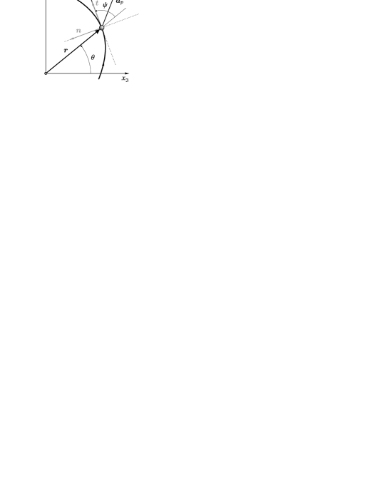
The gravitational acceleration written in the intrinsic frame , with
| (2.4) |
defined in terms of the velocity and angular momentum vectors, v and h respectively, reads
| (2.5) |
The flight-direction angle is given by
| (2.6) |
Consequently, perturbations of the form result in
| (2.7) |
Since the component normal to the velocity does not perform any work, Bacon (1959) neglected its contribution and found that
| (2.8) |
furnishes another integrable problem: the trajectory of the particle is a logarithmic spiral.
Motivated by this line of thought, we can treat the normal component of the acceleration in Eq. (2.7) separately by introducing a second parameter, :
| (2.9) |
The dimensionless parameters and are assumed constant. The forcing parameter controls the power exerted by the perturbation,
| (2.10) |
with the Keplerian energy of the system. The second parameter scales the terms that do not perform any work. Introducing the accelerations (2.5) and (2.9) into Eq. (2.1) yields
| (2.11) |
having replaced by the new parameter
| (2.12) |
Since the motion is planar we shall introduce a system of polar coordinates to formulate the problem. The radial velocity is defined as
| (2.13) |
whereas the projection of the velocity normal to the radiusvector takes the form
| (2.14) |
Consequently, these geometric relations unveil the dynamical equations:
| (2.15) |
The dynamics are referred to an inertial frame , with and using the -axis as the origin of angles. Figure 1 depicts the configuration of the problem. We restrict the study to prograde motions () without losing generality.
2.1 Similarity transformation
Consider a linear transformation of the form
| (2.16) |
defined explicitly by the positive constants , , and :
| (2.17) |
The constants , , and have units of length, time, and velocity, respectively. The symbol denotes derivatives with respect to , whereas is reserved for derivatives with respect to . The scaling factor can be seen as the ratio of a homothetic transformation that simply dilates or contracts the orbit. Similarly, represents a time dilation or contraction. The velocity of the particle transforms into
| (2.18) |
In addition, and are defined in terms of by virtue of
| (2.19) |
We assume and for consistency.
Equation (2.11) then becomes
| (2.20) |
which is equivalent to the normalized two-body problem
| (2.21) |
perturbed by the purely tangential acceleration
| (2.22) |
This result shows that establishes a similarity transformation between the two-body problem (2.1) perturbed by the acceleration (2.9), and the simpler problem in Eq. (2.21) and perturbed by (2.22). That is, transforms the solution to Eq. (2.20), , into the solution to Eq. (2.11), .
Using and as the generalized coordinates and velocities, respectively, the dynamics of the problem abide by the Euler-Lagrange equations
| (2.23) |
The Lagrangian of the transformed system takes the form
| (2.24) |
and the generalized forces read
| (2.25) |
2.2 Integrals of motion and dynamical symmetries
Let us introduce an infinitesimal transformation :
| (2.26) |
defined in terms of a small parameter and the generators and . For transformations that leave the action unchanged up to an exact differential,
| (2.27) |
with a given gauge, Noether’s theorem states that
| (2.28) |
is a first integral of the problem. Here is a certain constant of motion. We refer the reader to the work of Efroimsky and Goldreich (2004) for a refreshing look into the role of gauge functions in celestial mechanics.
Since the perturbation in Eq. (2.22) is not conservative, we shall focus on the extension of Noether’s theorem to nonconservative systems by Djukic and Vujanovic (1975). It must be for the conservation law to hold (Vujanovic et al., 1986). For the case of nonconservative systems the generators , , and the gauge need to satisfy the following relation:
| (2.29) |
This equation and the condition furnish the generalized Noether-Bessel-Hagen (NBH) equations (Trautman, 1967; Djukic and Vujanovic, 1975; Vujanovic et al., 1986). The NBH equations involve the full derivative of the gauge function and the generators with respect to , meaning that Eq. (2.29) depends on the partial derivatives of , , and with respect to time, the coordinates, and the velocities. By expanding the convective terms the NBH equations decompose in the system of Killing equations:
| (2.30) |
The system (2.30) decomposes in three equations that can be solved for the generators , , and given a certain gauge. If the transformation defined in Eq. (2.26) satisfies the NBH equations, then the system admits the integral of motion (2.28).
2.2.1 Generalized equation of the energy
The Lagrangian in Eq. (2.24) is time-independent. Thus, the action is not affected by arbitrary time transformations. In the Keplerian case a simple time translation reveals the conservation of the energy. Motivated by this fact, we explore the generators
| (2.31) |
Solving Killing equations (2.30) with the above generators leads to the gauge function
| (2.32) |
Provided that the NBH equations hold, the system admits the integral of motion
| (2.33) |
written in terms of the constant . This term can be solved from the initial conditions
| (2.34) |
When the perturbation (2.22) vanishes and Eq. (2.33) reduces to the normalized equation of the Keplerian energy. In fact, in this case becomes twice the Keplerian energy of the system, . Moreover, the gauge vanishes and Eq. (2.28) furnishes the Hamiltonian of Kepler’s problem. The integral of motion (2.33) is a generalization of the equation of the energy.
In the Keplerian case ( and ) the sign of the energy determines the type of solution. Negative values of yield elliptic orbits, positive values correspond to hyperbolas, and the orbits are parabolic for vanishing . We shall extend this classification to the general case : the solutions will be classified as elliptic (), parabolic (), and hyperbolic () orbits.
2.2.2 Generalized equation of the angular momentum
In the unperturbed problem is an ignorable coordinate. Indeed, a simple translation in (a rotation) with and yields the conservation of the angular momentum. In order to extend this first integral to the perturbed case, we consider the same generator . However, solving for the gauge and the remaining generators in Killing equations yields the nontrivial functions
| (2.35) |
They satisfy . Noether’s theorem holds and Eq. (2.28) furnishes the integral of motion
| (2.36) |
This first integral is none other than a generalized form of the conservation of the angular momentum. Indeed, making Eq. (2.36) reduces to
| (2.37) |
where coincides with the angular momentum of the particle. In addition, the generators and , and the gauge vanish when equals unity.
By recovering Eq. (2.15) the integral of motion (2.36) can be written:
| (2.38) |
in terms of the coordinates intrinsic to the trajectory. The fact that forces
| (2.39) |
The second step is possible because all variables are positive. Combining this expression with Eq. (2.33) yields
| (2.40) |
Depending on the values of , Eq. (2.40) may define upper or lower limits to the values that the radius can reach. In general, this condition can be resorted to provide the polynomial constraint
| (2.41) |
where is a polynomial of degree in whose roots dictate the nature of the solutions. This inequality will be useful for defining the different families of orbits.
2.3 Properties of the similarity transformation
The main property of the similarity transformation is that it does not change the type of the solution, i.e. the sign of is not altered. Applying the inverse similarity transformation to Eq. (2.33) yields
| (2.42) |
and results in
| (2.43) |
Since no matter the values of or , the sign of is not affected by the transformation . If the solution to the original problem (2.1) is elliptic, the solution to the reduced problem (2.21) will be elliptic too, and vice-versa. The transformation reduces to a series of scaling factors affecting each variable independently.
The integral of the angular momentum transforms into
| (2.44) |
The constant remains positive, although the scaling factor can modify its value significantly.
The transformation is defined in terms of three parameters: , and . For , with
| (2.45) |
reduces to the identity map. Choosing the special values of that yield trivial transformations for , , and are, respectively, , , and . The similarity transformation can be understood from a different approach: solving the simplified problem (2.20) is equivalent to solving the full problem (2.11), but setting .
Combining Eqs. (2.15) renders
| (2.46) |
The right-hand side of this equation can be written as a function of alone thanks to
| (2.47) |
The parameter is for orbits in a raising regime (), and for a lowering regime (). The velocity is solved from Eq. (2.33). Integrating Eq. (2.46) furnishes the solution , which can then be inverted to define the trajectory .
2.4 Solvability
The trajectory of the particle is obtained upon integration and inversion of Eq. (2.46). This equation can be written
| (2.48) |
where is a polynomial in , in particular
| (2.49) |
The roots of determine the form of the solution and coincide with those of (obviating the trivial ones). The integration of Eq. (2.48) depends on the factorization of . This polynomial expression can be expanded thanks to the binomial theorem:
| (2.50) |
with an integer. For the polynomial is of degree four: when or there are two trivial roots and Eq. (2.48) can be integrated using elementary functions; when or it yields elliptic integrals. Negative values of or positive values greater than four lead to a polynomial with degree five or above. The solution can no longer be reduced to elementary functions nor elliptic integrals (Whittaker and Watson, 1927, p. 512), for it is given by hyperelliptic integrals. This special class of Abelian integrals can only be inverted in very specific situations (see Byrd and Friedman, 1954, pp. 252–271). Thus, we shall focus on the solutions to the cases , , and .
The following sections 3–6 present the corresponding families of orbits. For the solutions to the reduced problem are Keplerian orbits. For the case the solutions are called generalized logarithmic spirals, because for the particle describes a logarithmic spiral (Roa et al., 2016a). The cases and yield generalized cardioids and generalized sinusoidal spirals, respectively (for the orbits are cardioids and sinusoidal spirals).
3 Case : conic sections
For the integrals of motion (2.33) and (2.36) reduce to the normalized equations of the energy and angular momentum, respectively. The condition on the radius given by Eq. (2.40) becomes
| (3.1) |
For the case (elliptic solution) this translates into , where
| (3.2) |
These limits are none other than the periapsis and apoapsis radii, provided that and relate to the semimajor axis and eccentricity by means of:
| (3.3) |
For (parabolic case) the semimajor axis becomes infinite, and Eq. (3.1) has only one root corresponding to . Note that it must be . Similarly, for hyperbolic orbits () it is as becomes negative.
Thus, the solution is simply a conic section:
| (3.4) |
The angle defines the direction of the line of apses in frame , meaning that is the true anomaly. If , then , and . The velocity follows from the integral of the energy:
| (3.5) |
It is minimum at apoapsis and maximum at periapsis.
Applying the similarity transformation to the previous solution leads to the extended integral
| (3.6) |
The factor behaves as a modified gravitational parameter. This kind of solutions arise from, for example, the effect of the solar radiation pressure directed along the Sun-line on a particle following a heliocentric orbit (McInnes, 2004, p. 121).
4 Case : generalized logarithmic spirals
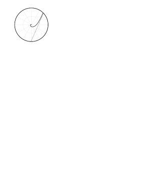
The case yields the family of generalized logarithmic spirals found by Roa et al. (2016a) in the context of interplanetary mission design. An extended version and the solution to the spiral Lambert problem can be found in following sequels (Roa and Peláez, 2016; Roa et al., 2016b). Negative values of define the so called elliptic spirals, positive values yield hyperbolic spirals, and the limit case corresponds to parabolic spirals, which turn out to be pure logarithmic spirals.
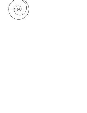
4.1 Elliptic motion
For the case the inequality in Eq. (2.40) translates into , with
| (4.1) |
Here behaves as the apoapsis of the elliptic spiral. In addition, it forces . Spirals of this type initially in raising regime will reach , then transition to lowering regime and fall toward the origin. If they are initially in lowering regime the radius will decrease monotonically. The velocity at apoapsis is the minimum possible velocity, and reads
| (4.2) |
Introducing the spiral anomaly :
| (4.3) |
and with , Eq. (2.46) can be integrated and inverted to provide the equation of the trajectory:
| (4.4) |
The angle defines the orientation of the apoapsis, i.e. . It can be solved form the initial conditions:
| (4.5) |
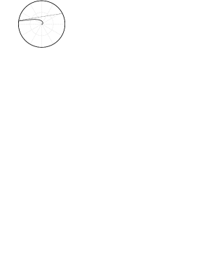
The trajectory is symmetric with respect to , provided that , and it is plotted in Fig. 2a (see Roa, 2016, Chap. 9, for details on the symmetry properties).
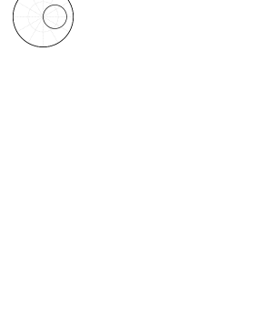
4.2 Parabolic motion: the logarithmic spiral
For parabolic spirals Eq. (2.40) reduces to , meaning that there are no limit radii. Spirals in raising regime escape to infinity, and spirals in lowering regime fall to the origin. The limit shows that the particle reaches infinity along a spiral branch.
The particle follows a pure logarithmic spiral,
| (4.6) |
keeping in mind that . See Fig. 2b for an example. In the reduced problem the velocity matches the local circular velocity, , and the parameter modifies the velocity in the full problem:
| (4.7) |
Note that when (or ) this is the true circular velocity.
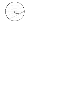
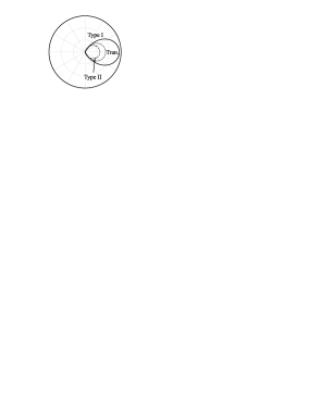
4.3 Hyperbolic motion
Under the assumption the polynomial constraint in Eq. (2.40) transforms into , with
| (4.8) |
This equation yields two different cases: when the periapsis radius becomes negative, which means that the spiral reaches the origin when in lowering regime. Conversely, for there is an actual periapsis; a spiral in lowering regime will reach , then transition to raising regime and escape. Hyperbolic spirals with are of Type I, whereas defines hyperbolic spirals of Type II.
Hyperbolic spirals reach infinity with a finite, nonzero velocity . That is, the generalized constant of the energy is equivalent to the characteristic energy .
4.3.1 Hyperbolic spirals of Type I
The trajectory described by a hyperbolic spiral with (Type I) takes the form
| (4.9) |
In this case the spiral anomaly reads
| (4.10) |
where the direction of the asymptote is solved from
| (4.11) |
An example of a Type I hyperbolic spiral connecting the origin with infinity can be found in Fig. 2c. The dashed line represents the asymptote.
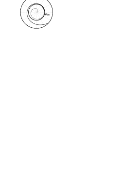
4.3.2 Hyperbolic spirals of Type II
Hyperbolic spirals of Type II are defined by
| (4.12) |
The spiral anomaly is defined in Eq. (4.3), with . The line of apses follows the direction of
| (4.13) |
Equation (4.12) depends on the spiral anomaly by means of . Thus, the trajectory is symmetric with respect to : the apse line is the axis of symmetry. The symmetry of the trajectory proves that there are two values of that cancel the denominator: there are two asymptotes, defined explicitly by
| (4.14) |
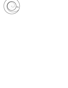
Both asymptotes are symmetric with respect to the line of apses. The shape of the hyperbolic spirals of Type II can be analyzed in Fig. 2d. The figure includes a zoomed view of the periapsis region.
4.3.3 Transition between Type I and Type II hyperbolic spirals
Hyperbolic spirals of Type I have been defined for , whereas yields hyperbolic spirals of Type II. In the limit case the equations of motion simplify noticeably; the resulting spiral is
| (4.15) |
The angular variable is defined with respect to the orientation of the asymptote, i.e.
| (4.16) |
The asymptote is fixed by
| (4.17) |
Qualitatively, this type of solution is equivalent to a Type II spiral with . The trajectory is similar to Type I spirals, or to one half of a Type II spiral (see Fig. 2e).
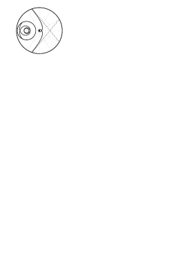
5 Case : Generalized cardioids
The condition in Eq. (2.40), yields the polynomial inequality:
| (5.1) |
The discriminant of the polynomial predicts the nature of the roots. It is
| (5.2) |
The intermediate value theorem shows that there is at least one real root. For the elliptic case it is , meaning that the other two roots are complex conjugates. In the hyperbolic case the sign of the discriminant depends on the values of : if it is , and for the discriminant is negative. This behavior yields two types of hyperbolic solutions.
5.1 Elliptic motion
The nature of elliptic motion is determined by the polynomial constraint in Eq. (5.1). The only real root is given by
| (5.3) |
with
| (5.4) |
Equation (5.1) reduces to and we shall write
| (5.5) |
Thus, elliptic generalized cardioids never escape to infinity because they are bounded by . When in raising regime they reach the apoapsis radius , then transition to lowering regime and fall toward the origin. The velocity at apoapsis,
| (5.6) |
is the minimum velocity in the cardioid.
Equation (2.46) can be integrated from the initial radius to the apoapsis of the cardioid, and the result provides the orientation of the line of apses:
| (5.7) |
where and are the complete and incomplete elliptic integrals of the first kind, respectively. Introducing the auxiliary term
| (5.8) |
their argument and modulus read
| (5.9) |
The previous definitions involve the auxiliary parameters:
| (5.10) |
and
| (5.11) |
Recall the definition of in Eq. (5.4).
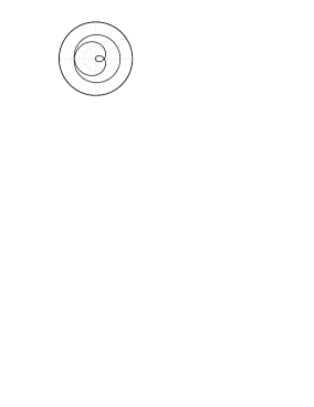
5.2 Parabolic motion: the cardioid
When the constant of the generalized energy vanishes the condition in Eq. (2.40) translates into , where the maximum radius takes the form
| (5.14) |
Parabolic generalized cardioids, unlike logarithmic spirals or Keplerian parabolas, are bounded (they never escape the gravitational attraction of the central body).
The line of apses is defined by:
| (5.15) |
The equation of the trajectory reveals that the orbit is in fact a pure cardioid:222The cardioid is a particular case of the limaçons, curves first studied by the amateur mathematician Étienne Pascal in the 17th century. The general form of the limaçon in polar coordinates is . Depending on the values of the coefficients the curve might reach the origin and form loops. It is worth noticing that the inverse of a limaçon, , results in a conic section. Limaçons with are considered part of the family of sinusoidal spirals.
| (5.16) |
This curve is symmetric with respect to . Figure 3b depicts the geometry of the solution.

5.3 Hyperbolic motion
The inequality in Eq. (2.40) determines the structure of the solutions and the sign of the discriminant (5.2) governs the nature of its roots. There are two types of hyperbolic generalized cardioids: for the cardioids are of Type I, and for the cardioids are of Type II.
5.3.1 Hyperbolic cardioids of Type I
For hyperbolic cardioids of Type I there is only one real root. The other two are complex conjugates. The real root is
| (5.17) |
having introduced the auxiliary parameter
| (5.18) |
Provided that , Eq. (5.17) shows that . Therefore, there are no limits to the values that can take. As a consequence, the cardioid never transitions between regimes. If it is initially it will always escape to infinity, and fall toward the origin for .
The equation of the trajectory for hyperbolic generalized cardioids of Type I is
| (5.19) |
It is defined in terms of
| (5.20) |
which require
| (5.21) |
There are no axes of symmetry. Therefore, the anomaly is referred directly to the initial conditions:
| (5.22) |
The moduli of both the Jacobi elliptic functions and the elliptic integral, and the argument of the latter, are
| (5.23) |
The cardioid approaches infinity along an asymptotic branch, with as . The orientation of the asymptote follows from the limit
| (5.24) |
Here, the value of ,
| (5.25) |
is defined as . An example of a hyperbolic cardioid of Type I with its corresponding asymptote is presented in Fig. 3c.
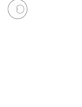
5.3.2 Hyperbolic cardioids of Type II
For hyperbolic cardioids of Type II the polynomial in Eq. (2.40) admits three distinct real roots, , given by
| (5.26) |
with . The roots are then sorted so that . Since
| (5.27) |
then and also for physical coherence. The polynomial constraint reads
| (5.28) |
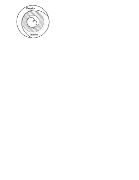
and holds for both and . The integral of motion (2.33) shows that both situations are physically admissible, because and . There are two families of solutions that lie outside the annulus . When the spirals are interior, whereas for they are exterior spirals. The geometry of the forbidden region can be analyzed in Fig. 3d. The particle cannot enter the barred annulus, whose limits coincide with the periapsis and apoapsis of the exterior and interior orbits, respectively.
The axis of symmetry of interior spirals is given by
| (5.29) |
in terms of the arguments:
| (5.30) |
The trajectory simplifies to:
| (5.31) |
Here we made use of Glaisher’s notation for the Jacobi elliptic functions,333Glaisher’s notation establishes that if p,q,r are any of the four letters s,c,d,n, then: (5.32) Under this notation repeated letters yield unity. so . The spiral anomaly takes the form
| (5.33) |
The trajectory is symmetric with respect to the line of apses defined by .
For the case of exterior spirals the largest root behaves as the periapsis. A cardioid initially in lowering regime will reach , then it will transition to raising regime and escape to infinity. Equation (2.46) is integrated from the initial radius to the periapsis to provide the orientation of the line of apses:
| (5.34) |
with
| (5.35) |
the argument and modulus of the elliptic integral.
The trajectory of exterior spirals is obtained upon inversion of the equation for the polar angle,
| (5.36) |
The anomaly is redefined as
| (5.37) |
This variable is referred to the line of apses, given in Eq. (5.34). The form of the solution shows that hyperbolic generalized cardioids of Type II are symmetric with respect to .
Due to the symmetry of Eq. (5.36) the trajectory exhibits two symmetric asymptotes, defined by
| (5.38) |
The argument reads
| (5.39) |
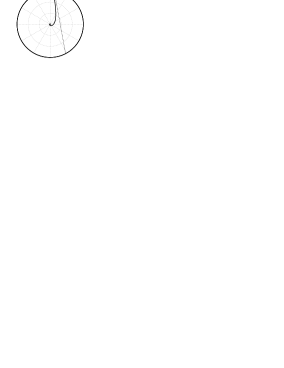
5.3.3 Transition between Type I and Type II hyperbolic cardioids
The limit case defines the transition between hyperbolic cardioids of Types I and II. The discriminant vanishes: the roots are all real and one is a multiple root, . The region of forbidden motion degenerates into a circumference of radius . The roots take the form:
| (5.40) |
The condition holds naturally for . When the cardioid reaches the velocity becomes . It coincides with the local circular velocity. Moreover, from the integral of motion (2.36) one has
| (5.41) |
meaning that the orbit becomes circular as the particle approaches . When the perturbing acceleration in Eq. (2.22) vanishes. As a result, the orbit degenerates into a circular Keplerian orbit. A cardioid with and in raising regime will reach and degenerate into a circular orbit with radius . This phenomenon also appears in cardioids with and in lowering regime.
The trajectory reduces to
| (5.42) |
which is written in terms of the anomaly
| (5.43) |
The integer determines whether the particle is initially below or above the limit radius . The limit shows that the radius converges to . This limit only applies to the cases and . When the particle is initially below and in lowering regime, , it falls toward the origin. In the opposite case, , the cardioid approaches infinity along an asymptotic branch with
| (5.44) |
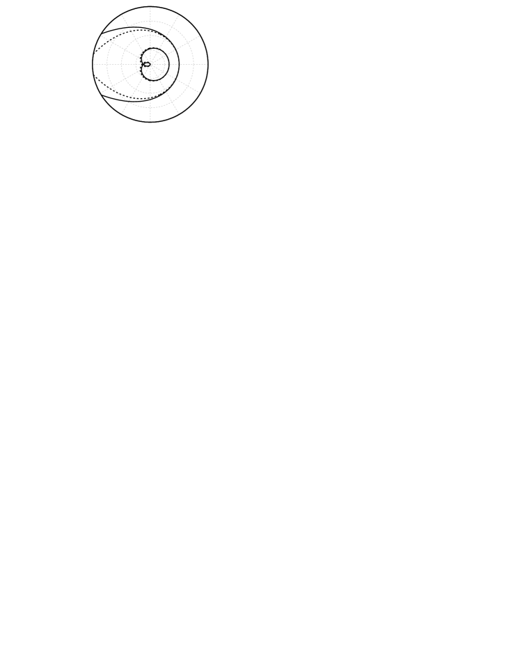
Two example trajectories with are plotted in Fig. 3e. The dashed line corresponds to and the solid line to . The trajectories terminate/emanate from a circular orbit of radius .
6 Case : generalized sinusoidal spirals
Setting in Eq. (2.40) gives rise to the polynomial inequality
| (6.1) |
which governs the subfamilies of the solutions to the problem. The four roots of the polynomial are
| (6.2) |
and the discriminant of is
| (6.3) |
The sign of the discriminant determines the nature of the four roots.
6.1 Elliptic motion
When there are two subfamilies of elliptic sinusoidal spirals: of Type I, with (), and of Type II, with (). Both types are separated by the limit case , which makes .
6.1.1 Elliptic sinusoidal spirals of Type I
For the case the discriminant is positive and the four roots are real, with . Since Eq. (6.1) reduces to
| (6.4) |
meaning that it must be either or . The integral of motion (2.33) reveals that only the latter case is physically possible, because . Thus, is the apoapsis of the spiral:
| (6.5) |
and . Equation (2.48) is then integrated from to to define the orientation of the apoapsis,
| (6.6) |
The arguments of the elliptic integrals are
| (6.7) |
Recall that .
Elliptic sinusoidal spirals of Type I are defined by
| (6.8) |
The spiral anomaly reads
| (6.9) |
The trajectory is symmetric with respect to , which corresponds to the line of apses.
6.1.2 Elliptic sinusoidal spirals of Type II
When two roots are real and the other two are complex conjugates. In this case the real roots are and the inequality (6.1) reduces again to Eq. (6.4), meaning that . However, the form of the solution is different from the trajectory described by Eq. (6.8), being
| (6.10) |
The spiral anomaly is
| (6.11) |
It is referred to the orientation of the apse line, . This variable is given by
| (6.12) |
considering the arguments:
| (6.13) |
The coefficients and are defined in terms of
| (6.14) |
namely
| (6.15) |
The fact that the Jacobi function is symmetric proves that elliptic sinusoidal spirals of Type II are symmetric.
6.1.3 Transition between spirals of Types I and II
In this is particular case of elliptic motion, , the roots of polynomial are
| (6.16) |
These results simplify the definition of the line of apses to
| (6.17) |
Introducing the spiral anomaly ,
| (6.18) |
the equation of the trajectory takes the form
| (6.19) |
The trajectory is symmetric with respect to the line of apses thanks to the symmetry of the hyperbolic cosine.
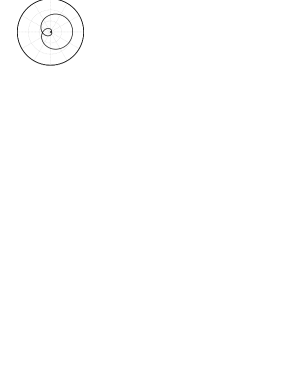
6.2 Parabolic motion: sinusoidal spiral (off-center circle)
Making , the condition in Eq. (6.1) simplifies to
| (6.20) |
meaning that the spiral is bounded by a maximum radius . It is equivalent to the apoapsis of the spiral. Its orientation is given by
| (6.21) |
The trajectory reduces to a sinusoidal spiral,444It was the Scottish mathematician Colin Maclaurin the first to study sinusoidal spirals. In his “Tractatus de Curvarum Constructione & Mensura”, published in Philosophical Transactions in 1717, he constructed this family of curves relying on the epicycloid. Their general form is and different values of render different types of curves; correspond to hyperbolas, to straight lines, to parabolas, to Tschirnhausen cubics, to Cayley’s sextics, to cardioids, to circles, and to lemniscates. and its definition can be directly related to :
| (6.22) |
The spiral defined in Eq. (6.22) is symmetric with respect to the line of apses. The resulting orbit is a circle centered at (Fig. 4b). Circles are indeed a special case of sinusoidal spirals.
6.3 Hyperbolic motion
Given the discriminant in Eq. (6.3), for the case the values of the constant define two different types of hyperbolic sinusoidal spirals: spirals of Type I (), and spirals of Type II ().
6.3.1 Hyperbolic sinusoidal spirals of Type I
If , then are complex conjugates and are both real but negative. Therefore, the condition in Eq. (6.1) holds naturally for any radius and there are no limitations to the values of . The particle can either fall to the origin or escape to infinity along an asymptotic branch. The equation of the trajectory is given by:
| (6.23) |
where the spiral anomaly can be referred directly to the initial conditions:
| (6.24) |
This definition involves an elliptic integral of the first kind with argument and parameter:
| (6.25) |
The coefficients and require the terms:
| (6.26) |
being
| (6.27) |
The direction of the asymptote is defined by
| (6.28) |
This definition involves the argument
| (6.29) |
The velocity of the particle when reaching infinity is . Hyperbolic sinusoidal spirals of Type I are similar to the hyperbolic solutions of Type I with and . Figure 4d depicts and example trajectory and the asymptote defined by .
6.3.2 Hyperbolic sinusoidal spirals of Type II
In this case the four roots are real and distinct, with . The two positive roots are physically valid, i.e. and . This yields two situations in which the condition is satisfied: (exterior spirals) and (interior spirals).
Interior spirals take the form
| (6.30) |
The spiral anomaly is
| (6.31) |
The orientation of the line of apses is solved from
| (6.32) |
with
| (6.33) |
Interior hyperbolic spirals are bounded and their shape is similar to that of a limaçon.
The line of apses of an exterior spiral is defined by
| (6.34) |
The modulus and the argument of the elliptic integral are
| (6.35) |
The trajectory becomes
| (6.36) |
and it is symmetric with respect to . The geometry of the solution is similar to that of hyperbolic cardioids of Type II, mainly because of the existence of the forbidden region plotted in Fig. 4d. The asymptotes follow the direction of
| (6.37) |
6.3.3 Transition between Type I and Type II spirals
When the radii and coincide, , and become equal to the limit radius
| (6.38) |
The equation of the trajectory is a particular case of Eq. (6.36), obtained with :
| (6.39) |
The spiral anomaly can be referred to the initial conditions,
| (6.40) |
avoiding additional parameters. Here determines whether the spiral is below or over the limit radius . The asymptote follows from
| (6.41) |
Like in the case of hyperbolic cardioids, for and spirals of this type approach the circular orbit of radius asymptotically, i.e. . When approaching a circular orbit the perturbing acceleration vanishes and the spiral converges to a Keplerian orbit. See Fig. 4e for examples of hyperbolic sinusoidal spirals with (dashed) and (solid).
7 Summary
The solutions presented in the previous sections are summarized in Table 1, organized in terms of the values of . Each family is then divided in elliptic, parabolic, and hyperbolic orbits. The table includes references to the corresponding equations of the trajectories for convenience. The orbits are said to be bounded if the particle can never reach infinity, because .
| Family | Type | Bounded | Trajectory | |||
| Elliptic | 1 | Y | Eq. (3.4) | |||
| Conic sections | Parabolic | 1 | N | Eq. (3.4) | ||
| Hyperbolic | 1 | N | Eq. (3.4) | |||
| Elliptic | 2 | Y | Eq. (4.4) | |||
| Generalized | Parabolic | 2 | N | Eq. (4.6)∗ | ||
| logarithmic | Hyperbolic T-I | 2 | N | Eq. (4.9) | ||
| spirals | Hyperbolic T-II | 2 | N | Eq. (4.12) | ||
| Hyperbolic trans. | 2 | N | Eq. (4.15) | |||
| Elliptic | 3 | Y | Eq. (5.12) | |||
| Parabolic | 3 | Y | Eq. (5.16)† | |||
| Generalized | Hyperbolic T-I | 3 | N | Eq. (5.19) | ||
| cardioids | Hyperbolic T-II (int) | 3 | Y | Eq. (5.31) | ||
| Hyperbolic T-II (ext) | 3 | N | Eq. (5.36) | |||
| Hyperbolic trans. | 3 | Y/N | Eq. (5.42) | |||
| Elliptic T-I | 4 | Y | Eq. (6.8) | |||
| Elliptic T-II | 4 | Y | Eq. (6.10) | |||
| Generalized | Elliptic trans. | 4 | Y | Eq. (6.19) | ||
| sinusoidal | Parabolic | 4 | Y | Eq. (6.22)‡ | ||
| spirals | Hyperbolic T-I | 4 | N | Eq. (6.23) | ||
| Hyperbolic T-II (int) | 4 | Y | Eq. (6.30) | |||
| Hyperbolic T-II (ext) | 4 | N | Eq. (6.36) | |||
| Hyperbolic trans. | 4 | Y/N | Eq. (6.39) |
∗ Logarithmic spiral.
† Cardioid.
‡ Sinusoidal spiral (off-center circle).
8 Unified solution in Weierstrassian formalism
The orbits can be unified introducing the Weierstrass elliptic functions. Indeed, Eq. (2.48) furnishes the integral expression
| (8.1) |
with
| (8.2) |
and . Introducing the auxiliary parameters
| (8.3) |
Eq. (8.1) can be inverted to provide the equation of the trajectory (Whittaker and Watson, 1927, p. 454),
| (8.4) |
The solution is written in terms of the Weierstrass elliptic function
| (8.5) |
and its derivative , where is the argument and the invariant lattices and read
| (8.6) |
The coefficients and are obtained by identifying Eq. (8.1) with Eq. (2.48) for different values of . They can be found in Table 2.
| 1 | 1/2 | 0 | 0 | |||
|---|---|---|---|---|---|---|
| 2 | 0 | 0 | ||||
| 3 | 2 | 0 | ||||
| 4 |
Symmetric spirals reach a minimum or maximum radius , which is a root of . Thus, Eq. (8.4) can be simplified if referred to instead of :
| (8.7) |
This is the unified solution for all symmetric solutions, with . Practical comments on the implementation of the Weierstrass elliptic functions can be found in Biscani and Izzo (2014), for example. Although , the derivative is an odd function in , . Therefore, the integer needs to be adjusted according to the regime of the spiral when solving Eq. (8.4): for raising regime, and for lowering regime.
9 Physical discussion of the solutions
Each family of solutions involves a fundamental curve: the case relates to conic sections, to logarithmic spirals, to cardioids, and to sinusoidal spirals. This section is devoted to analyzing the geometrical and dynamical connections between the solutions and other integrable systems.
9.1 Connection with Schwarzschild geodesics
The Schwarzschild metric is a solution to the Einstein field equations of the form
| (9.1) |
written in natural units so that the speed of light and the gravitational constant equal unity, and the Schwarzschild radius reduces to . In this equation is the mass of the central body, is the colatitude, and is the longitude.
The time-like geodesics are governed by the differential equation
| (9.2) |
where is the angular momentum and is a constant of motion related to the energy and defined by
| (9.3) |
in terms of the proper time of the particle and the Schwarzschild time . Its solution is given by
| (9.4) |
and involves the integer , which gives the raising/lowering regime of the solution. Here is a quartic function defined like in Eq. (8.2). The previous equation is formally equivalent to Eq. (8.1). As a result, the Schwarzschild geodesics abide by Eqs. (8.4) or (8.7), which are written in terms of the Weierstrass elliptic functions and identifying the coefficients
| (9.5) |
Compact forms of the Schwarzschild geodesics using the Weierstrass elliptic functions can be found in the literature (see for example Hagihara, 1930, §4). We refer to classical books like the one by Chandrasekhar (1983, Chap. 3) for an analysis of the structure of the solutions in Schwarzschild metric.
The analytic solution to Schwarzschild geodesics involves elliptic functions, like generalized cardioids () and generalized sinusoidal spirals (). If the values of and are adjusted in order the roots of to coincide with the roots of in Schwarzschild metric, the solutions will be comparable. For example, when the polynomial has three real roots and a repeated one the geodesics spiral toward or away from the limit radius
| (9.6) |
If we make this radius coincide with the limit radius of a hyperbolic cardioid with [Eq. (5.40)] it follows
| (9.7) |
Figure 5a compares hyperbolic generalized cardioids and Schwarzschild geodesics with the same limit radius. The interior solutions coincide almost exactly, whereas exterior solutions separate slightly. Similarly, when admits three real and distinct roots the geodesics are comparable to interior and exterior hyperbolic solutions of Type II. For example, Fig. 5b shows interior and exterior hyperbolic sinusoidal spirals of Type II with the inner and outer radii equal to the limit radii of Schwarzschild geodesics. Like in the previous example the interior solutions coincide, while the exterior solutions separate in time. In order for two completely different forces to yield a similar trajectory it suffices that the differential equation takes the same form. Even if the trajectory is similar the integrals of motion might not be comparable, because the angular velocities may be different. As a result, the velocity along the orbit and the time of flight between two points will be different. Equation (2.46) shows that the radial motion is governed by the evolution of the flight-direction angle. For and the acceleration in Eq. (2.22) makes the radius to evolve with the polar angle just like in the Schwarzschild metric. Consequently, the orbits may be comparable. However, since the integrals of motion (2.33) and (2.36) do not hold along the geodesics, the velocities will not necessarily match.

9.2 Newton’s theorem of revolving orbits
Newton found that if the angular velocity of a particle following a Keplerian orbit is multiplied by a constant factor , it is then possible to describe the dynamics by superposing a central force depending on an inverse cubic power of the radius. The additional perturbing terms depend only on the angular momentum of the original orbit and the value of .
Consider a Keplerian orbit defined as
| (9.8) |
Here denotes the true anomaly. The radial motion of hyperbolic spirals of Type II —Eq. (4.12)— resembles a Keplerian hyperbola. The difference between both orbits comes from the angular motion, because they revolve with different angular velocities. Indeed, recovering Eq. (4.12), identifying and , and calling the spiral anomaly , it is
| (9.9) |
When equated to Eq. (9.8), it follows a relation between the spiral () and the true () anomalies:
| (9.10) |
The factor reads
| (9.11) |
Replacing by in Eq. (9.8) and introducing the result in the equations of motion in polar coordinates gives rise to the radial acceleration that renders a hyperbolic generalized logarithmic spiral of Type II, namely
| (9.12) |
This is in fact the same result predicted by Newton’s theorem of revolving orbits.
The radial acceleration yields a hyperbolic generalized logarithmic spiral of Type II. This is a central force which preserves the angular momentum, but not the integral of motion in Eq. (2.36). Thus, a particle accelerated by describes the same trajectory as a particle accelerated by the perturbation in Eq. (2.22), but with different velocities. As a consequence, the times between two given points are also different. The acceleration derives from the specific potential
| (9.13) |
where denotes the Keplerian potential, and is the perturbing potential:
| (9.14) |
9.3 Geometrical and physical relations
The inverse of a generic conic section , using one of its foci as the center of inversion, defines a limaçon. In particular, the inverse of a parabola results in a cardioid. Let us recover the equation of the trajectory of a generalized parabolic cardioid (a true cardioid) from Eq. (5.16),
| (9.15) |
Taking the cusp as the inversion center defines the inverse curve:
| (9.16) |
Identifying the terms in this equation with the elements of a parabola it follows that the inverse of a generalized parabolic cardioid with apoapsis is a Keplerian parabola with periapsis . The axis of symmetry remains invariant under inversion; the lines of apses coincide.
The subfamily of elliptic generalized logarithmic spirals is a generalized form of Cotes’s spirals, more specifically of Poinsot’s spirals:
| (9.17) |
Cotes’s spirals are known to be the solution to the motion immerse in a potential (Danby, 1992, p. 69).
The radial motion of interior Type II hyperbolic and Type I elliptic sinusoidal spirals has the same form, and is also equal to that of Type II hyperbolic generalized cardioids, except for the sorting of the terms.
It is worth noticing that the dynamics along hyperbolic sinusoidal spirals with are qualitatively similar to the motion under a central force decreasing with . Indeed, the orbits shown in Fig. 4e behave as the limit case discussed by MacMillan (1908, Fig. 4). On the other hand, parabolic sinusoidal spirals (off-center circles) are also the solution to the motion under a central force proportional to .
10 Conclusions
The dynamical symmetries in Kepler’s problem hold under a special nonconservative perturbation: a disturbance that modifies the tangential and normal components of the gravitational acceleration in the intrinsic frame renders two integrals of motion, which are generalized forms of the equations of the energy and angular momentum. The existence of a similarity transformation that reduces the original problem to a system perturbed by a tangential uniparametric forcing simplifies the dynamics significantly, for the integrability of the system is evaluated in terms of one single parameter. The algebraic properties of the equations of motion dictate what values of the free parameter make the problem integrable in closed form.
The extended integrals of motion include the Keplerian ones as particular cases. The new conservation laws can be seen as generalizations of the original integrals. The new families of solutions are defined by fundamental curves in the zero-energy case, and there are geometric transformations that relate different orbits. The orbits can be unified by introducing the Weierstrass elliptic functions. This approach simplifies the modeling of the system.
The solutions derived in this paper are closely related to different physical problems. The fact that the magnitude of the acceleration decreases with makes it comparable with the perturbation due to the solar radiation pressure. Moreover, the inverse similarity transformation converts Keplerian orbits into the conic sections obtained when the solar radiation pressure is directed along the radial direction. The structure of the solutions, governed by the roots of a polynomial, is similar in nature to the Schwarzschild geodesics. This is because under the considered perturbation and in Schwarzschild metric the evolution of the radial distance takes the same form. The perturbation can also be seen as a control law for a continuous-thrust propulsion system. Some of the solutions are comparable with the orbits deriving from potentials depending on different powers of the radial distance. Although the trajectory may take the same form, the velocity will be different, in general.
Acknowledgements
This work is part of the research project entitled “Dynamical Analysis, Advanced Orbit Propagation and Simulation of Complex Space Systems” (ESP2013-41634-P) supported by the Spanish Ministry of Economy and Competitiveness. The author has been funded by a “La Caixa” Doctoral Fellowship for he is deeply grateful to Obra Social “La Caixa”. The present paper would not have been possible without the selfless help, support, and advice from Prof. Jesús Peláez. An anonymous reviewer made valuable contributions to the final version of the manuscript.
References
- Adkins and McDonnell (2007) Adkins, GS., McDonnell, J. (2007) Orbital precession due to central-force perturbations. Phys Rev D 75(8):082,001
- Akella and Broucke (2002) Akella, MR., Broucke, RA. (2002) Anatomy of the constant radial thrust problem. J Guid Control Dynam 25(3):563–570
- Arnold et al. (2007) Arnold, VI., Kozlov, VV., Neishtadt, AI. (2007) Mathematical aspects of classical and celestial mechanics, 3rd edn. Springer
- Bacon (1959) Bacon, RH. (1959) Logarithmic spiral: An ideal trajectory for the interplanetary vehicle with engines of low sustained thrust. Am J Phys 27(3):164–165
- Bahar and Kwatny (1987) Bahar, LY., Kwatny, HG. (1987) Extension of Noether’s theorem to constrained non-conservative dynamical systems. Int J Nonlin Mech 22(2):125–138
- Basilakos et al. (2011) Basilakos, S., Tsamparlis, M., Paliathanasis, A. (2011) Using the Noether symmetry approach to probe the nature of dark energy. Phys Rev D 83(10):103,512
- Baù et al. (2015) Baù, G., Bombardelli, C., Peláez, J., Lorenzini, E. (2015) Non-singular orbital elements for special perturbations in the two-body problem. Mon Not R Astron Soc 454:2890–2908
- Beisert et al. (2008) Beisert, N., Ricci, R., Tseytlin, AA., Wolf, M. (2008) Dual superconformal symmetry from AdS superstring integrability. Phys Rev D 78(12):126,004
- Biscani and Carloni (2012) Biscani, F., Carloni, S. (2012) A first-order secular theory for the post-newtonian two-body problem with spin–i. the restricted case. Mon Not R Astron Soc p sts198
- Biscani and Izzo (2014) Biscani, F., Izzo, D. (2014) The Stark problem in the Weierstrassian formalism. Mon Not R Astron Soc p stt2501
- Broucke (1980) Broucke, R. (1980) Notes on the central force . Astrophys Space Sci 72(1):33–53
- Brouwer (1959) Brouwer, D. (1959) Solution of the problem of artificial satellite theory without drag. Astron J 64(1274):378–396
- Brouwer and Hori (1961) Brouwer, D., Hori, G. (1961) Theoretical evaluation of atmospheric drag effects in the motion of an artificial satellite. Astron J 66:193
- Byrd and Friedman (1954) Byrd, PF., Friedman, MD. (1954) Handbook of elliptic integrals for engineers and physicists. Springer
- Capozziello et al. (2009) Capozziello, S., Piedipalumbo, E., Rubano, C., Scudellaro, P. (2009) Noether symmetry approach in phantom quintessence cosmology. Phys Rev D 80(10):104,030
- Carpintero (2008) Carpintero, DD. (2008) Finding how many isolating integrals of motion an orbit obeys. Mon Not R Astron Soc 388(3):1293–1304
- Carpintero and Aguilar (1998) Carpintero, DD., Aguilar, LA. (1998) Orbit classification in arbitrary 2d and 3d potentials. Mon Not R Astron Soc 298(1):1–21
- Chandrasekhar (1983) Chandrasekhar, S. (1983) The Mathematical Theory of Black Holes. The International Series of Monographs on Physics, Oxford University Press
- Chandrasekhar (1995) Chandrasekhar, S. (1995) Newton’s Principia for the common reader. Oxford University Press
- Chashchina and Silagadze (2008) Chashchina, O., Silagadze, Z. (2008) Remark on orbital precession due to central-force perturbations. Phys Rev D 77(10):107,502
- Contopoulos (1967) Contopoulos, G. (1967) Integrals of motion in the elliptic restricted three-body problem. Astron J 72:669
- Danby (1992) Danby, J. (1992) Fundamentals of Celestial Mechanics, 2nd edn. Willman-Bell
- Djukic and Vujanovic (1975) Djukic, DDS., Vujanovic, B. (1975) Noether’s theory in classical nonconservative mechanics. Acta Mechanica 23(1-2):17–27
- Djukic and Sutela (1984) Djukic, DS., Sutela, T. (1984) Integrating factors and conservation laws for nonconservative dynamical systems. Int J Nonlin Mech 19(4):331–339
- Efroimsky and Goldreich (2004) Efroimsky, M., Goldreich, P. (2004) Gauge freedom in the N-body problem of celestial mechanics. Astron Astrophys 415(3):1187–1199
- Hagihara (1930) Hagihara, Y. (1930) Theory of the relativistic trajectories in a gravitational field of Schwarzschild. Japanese Journal of Astronomy and Geophysics 8:67
- Halpern et al. (1977) Halpern, M., Jevicki, A., Senjanović, P. (1977) Field theories in terms of particle-string variables: Spin, internal symmetries, and arbitrary dimension. Phys Rev D 16(8):2476
- Hénon and Heiles (1964) Hénon, M., Heiles, C. (1964) The applicability of the third integral of motion: some numerical experiments. Astron J 69:73
- Honein et al. (1991) Honein, T., Chien, N., Herrmann, G. (1991) On conservation laws for dissipative systems. Phys Lett A 155(4):223–224
- Izzo and Biscani (2015) Izzo, D., Biscani, F. (2015) Explicit solution to the constant radial acceleration problem. J Guid Control Dynam 38(4):733–739
- Lantoine and Russell (2011) Lantoine, G., Russell, RP. (2011) Complete closed-form solutions of the Stark problem. Celest Mech Dyn Astr 109(4):333–366
- MacMillan (1908) MacMillan, WD. (1908) The motion of a particle attracted towards a fixed center by a force varying inversely as the fifth power of the distance. Am J Math 30(3):282–306
- McInnes (2004) McInnes, CR. (2004) Solar sailing: technology, dynamics and mission applications. Springer Science & Business Media
- Narayan et al. (1987) Narayan, R., Goldreich, P., Goodman, J. (1987) Physics of modes in a differentially rotating system–analysis of the shearing sheet. Mon Not R Astron Soc 228(1):1–41
- Noether (1918) Noether, E. (1918) Invariante variationsprobleme. Nachr Akad Wiss Goett Math-Phys K1 II:235–257
- Olver (2000) Olver, PJ. (2000) Applications of Lie groups to differential equations, vol 107. Springer Science & Business Media
- Peláez et al. (2007) Peláez, J., Hedo, JM., de Andrés, PR. (2007) A special perturbation method in orbital dynamics. Celest Mech Dyn Astr 97(2):131–150
- Poincaré (1892) Poincaré, H. (1892) Les méthodes nouvelles de la Mécanique Céleste, vol 1. Paris: Gauthier-Villars et Fils
- Roa (2016) Roa, J. (2016) Regularization in astrodynamics: applications to relative motion, low-thrust missions, and orbit propagation. PhD thesis, Technical University of Madrid
- Roa and Peláez (2015) Roa, J., Peláez, J. (2015) Orbit propagation in Minkowskian geometry. Celest Mech Dyn Astr 123(1):13–43
- Roa and Peláez (2016) Roa, J., Peláez, J. (2016) Introducing a degree of freedom in the family of generalized logarithmic spirals. In: 26th Spaceflight Mechanics Meeting, 16-317
- Roa et al. (2015) Roa, J., Sanjurjo-Rivo, M., Peláez, J. (2015) Singularities in Dromo formulation. Analysis of deep flybys. Adv Space Res 56(3):569–581
- Roa et al. (2016a) Roa, J., Peláez, J., Senent, J. (2016a) New analytic solution with continuous thrust: generalized logarithmic spirals. J Guid Control Dynam
- Roa et al. (2016b) Roa, J., Peláez, J., Senent, J. (2016b) Spiral Lambert’s problem. J Guid Control Dynam
- San-Juan et al. (2012) San-Juan, JF., López, LM., Lara, M. (2012) On bounded satellite motion under constant radial propulsive acceleration. Math Probl Eng 2012
- Schmidt (2008) Schmidt, HJ. (2008) Perihelion precession for modified newtonian gravity. Phys Rev D 78(2):023,512
- Szebehely and Giacaglia (1964) Szebehely, V., Giacaglia, GE. (1964) On the elliptic restricted problem of three bodies. Astron J 69:230
- Trautman (1967) Trautman, A. (1967) Noether equations and conservation laws. Commun Math Phys 6(4):248–261
- Tsien (1953) Tsien, H. (1953) Take-off from satellite orbit. J Am Rocket Soc 23(4):233–236
- Urrutxua et al. (2015a) Urrutxua, H., Morante, D., Sanjurjo-Rivo, M., Peláez, J. (2015a) Dromo formulation for planar motions: solution to the Tsien problem. Celest Mech Dyn Astr 122(2):143–168
- Urrutxua et al. (2015b) Urrutxua, H., Sanjurjo-Rivo, M., Peláez, J. (2015b) Dromo propagator revisited. Celest Mech Dyn Astr 124(1):1–31
- Vujanovic et al. (1986) Vujanovic, B., Strauss, A., Jones, S. (1986) On some conservation laws of conservative and non-conservative dynamic systems. Int J Nonlin Mech 21(6):489–499
- Whittaker (1917) Whittaker, ET. (1917) Treatise on analytical dynamics of particles and rigid bodies, 2nd edn. Cambridge University Press
- Whittaker and Watson (1927) Whittaker, ET., Watson, GN. (1927) A course of modern analysis. Cambridge University Press
- Xia (1993) Xia, Z. (1993) Arnold diffusion in the elliptic restricted three-body problem. J Dyn Differ Equ 5(2):219–240
- Yoshida (1983a) Yoshida, H. (1983a) Necessary condition for the existence of algebraic first integrals I: Kowalevski’s exponents. Celestial Mech 31(4):363–379
- Yoshida (1983b) Yoshida, H. (1983b) Necessary condition for the existence of algebraic first integrals II: Condition for algebraic integrability. Celestial Mech 31(4):381–399
- Yukawa (1935) Yukawa, H. (1935) On the interaction of elementary particles. I. Proc Phys Math Soc Japan 17(0):48–57