Nonequilibrium spintronic transport through Kondo impurities
Abstract
In this work we analyze the nonequilibrium transport through a quantum impurity (quantum dot or molecule) attached to ferromagnetic leads by using a hybrid numerical renormalization group-time-dependent density matrix renormalization group thermofield quench approach.For this, we study the bias dependence of the differential conductance through the system, which shows a finite zero-bias peak, characteristic of the Kondo resonance and reminiscent of the equilibrium local density of states. In the non-equilibrium settings, the resonance in the differential conductance is also found to decrease with increasing the lead spin polarization. The latter induces an effective exchange field that lifts the spin degeneracy of the dot level. Therefore as we demonstrate, the Kondo resonance can be restored by counteracting the exchange field with a finite external magnetic field applied to the system. Finally, we investigate the influence of temperature on the nonequilibrium conductance, focusing on the split Kondo resonance. Our work thus provides an accurate quantitative description of the spin-resolved transport properties relevant for quantum dots and molecules embedded in magnetic tunnel junctions.
I Introduction
Charge and spin transport through nanostructures such as nanowires, quantum dots or molecules have been under rigorous experimental as well as theoretical research worldwide. These studies are motivated primarily by the possible applications in spintronics, nanoelectronics and spin caloritronics, as well as fascinating physics emerging at the nanoscale [1, 2, 3, 4]. In particular, the high research interest in transport through artificial quantum impurity systems stems from the observation of the Kondo effect, a many-body phenomenon, in which the spin of a quantum impurity becomes screened by conduction electrons of attached electrodes [5, 6, 7]. Many studies, both experimental and theoretical ones, focused on providing a deep understanding of the interplay between the Kondo physics and other many-body phenomena, such as e.g. ferromagnetism [8, 9] or superconductivity [10, 11], have been carried out. In this regard, especially interesting in the context of spin nanoelectronics, are quantum dots or molecules attached to ferromagnetic electrodes [12, 13]. Besides the fact that such nanostructures allow for implementing devices with high spin-resolved properties, they enable the exploration of the interplay between the itinerant ferromagnetism with the strong electron correlations [9, 14, 15, 16]. In fact, the spintronic transport properties of ferromagnetic quantum impurity systems have been a subject of extensive investigations [8, 17, 18, 9, 19, 20, 14, 15, 21, 16, 22, 23, 24, 25], however, their accurate quantitative description in truly nonequilibrium settings still poses a formidable challenge.
Reliable equilibrium and linear-response studies of transport through quantum impurity systems have been made possible by a robust non-perturbative numerical renormalization group (NRG) method [26, 27]. Unfortunately, this method falls short when describing the nonequilibrium behavior. On the other hand, although nonequilibrium situations can be studied by various analytical methods, their main drawback is an approximate treatment of electron correlations. It is important to note that these disadvantages have been overcome by the time-dependent density matrix renormalization group (tDMRG) method [28] which however has the drawback that it can only reliably study the system’s behavior for timescales of the order , where is the half-bandwidth of the conduction band. A reliable quantum quench approach to study the transport through quantum impurity systems out-of-equilibrium has been recently proposed by F. Schwarz et al. [29]. This approach combines both the NRG and tDMRG methods and, in addition, makes use of the thermofield treatment [30] to efficiently describe the system.
In this paper, by employing the hybrid NRG-tDMRG thermofield quench approach [29], we provide an accurate theoretical investigation of the nonequilibrium transport through a quantum impurity interacting with ferromagnetic leads. In particular, we study the bias voltage dependence of the differential conductance, which exhibits a zero-bias peak, a characteristic feature of the Kondo effect, when the system is tuned to the particle-hole symmetry point. We show that the Kondo energy scale in the applied bias potential decreases with increasing the lead spin polarization. On the other hand, when we detune the system away from this symmetry point, we observe a splitting of the zero-bias peak for finite lead spin polarization, which can be attributed to the emergence of a local exchange field in the impurity. Furthermore, we study the behavior of this split-Kondo peak under external parameters, such as applied magnetic field or temperature. We show that a particular value of the magnetic field can lead to the restoration of the Kondo resonance in the system. Moreover, we determine the temperature dependence of the differential conductance at the bias voltage corresponding to the split Kondo peak.
The paper is organized as follows. In Sec. II we describe the model and method used in calculations. Main results and their discussion are presented in Sec. III, where we first analyze the differential conductance at the particle-hole symmetry point, and then study the effect of finite exchange field on the transport behavior. We also examine the possibility to restore the Kondo effect by magnetic field and determine the temperature dependence. Finally, the paper is summarized in Sec. IV.
II Model and method
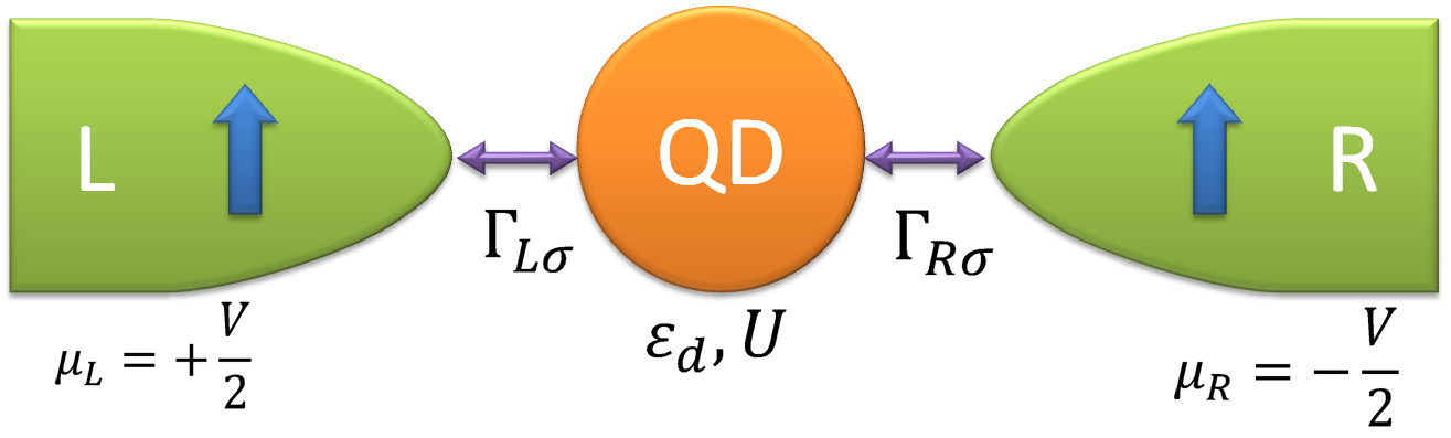
The considered system consists of a quantum impurity (quantum dot or a molecule) attached to two ferromagnetic leads with spin-dependent couplings, subject to a voltage bias, as shown schematically in Fig. 1. More specifically, such system can be described by a single impurity Anderson model [31], in which the quantum impurity is modeled as
| (1) |
with , where creates an electron with spin at the impurity, denotes the energy of an impurity energy level with the external magnetic field in units of , and the Coulomb repulsion experienced when the level is doubly occupied.
The leads attached to the impurity are assumed to be ferromagnetic metals and are characterized by the Fermi functions, (using units , throughout), where the index refers to the leads, and . The lead Hamiltonian reads as follows
| (2) |
with creating an electron in lead with energy , momentum , and spin . The quantum impurity is coupled to the leads according to the Hamiltonian ,
| (3) |
Electronic transition between each lead mode and the impurity spin state is specified by the tunnel matrix elements . This coupling between the lead and impurity induces an impurity-lead hybridization in the system, expressed by the hybridization function . Finally, the total Hamiltonian of the system reads,
| (4) |
In this work we assume a constant hybridization function over the entire bandwidth (we use as unit of energy throughout, unless specified otherwise). The hybridization function can thus be written as , with the Heaviside step function and constant , where is the spin-dependent density of states of lead . Assuming is independent of spin or lead, it is then convenient to introduce the spin polarization of the ferromagnetic contact ,
| (5) |
The coupling strength can be then written as , with . The total coupling strength for spin is given by, . In the following we assume that the system is left-right symmetric, i.e. and . Consequently, the computed electrical current through the impurity is independent of the sign of the applied bias voltage , and therefore it suffices to analyze .
The impurity parameters are fixed to
| (6) |
throughout our paper to ensure a well-defined Kondo regime well isolated from the finite bandwidth, with the impurity level position varied from particle-hole symmetric () to asymmetric ().
We use a hybrid NRG-tDMRG thermofield quench method [29] to study the non-equilibrium behavior of the system. This initializes the leads in thermal equilibrium at their respective chemical potentials, before they get dynamically coupled when smoothly turning on the coupling to the impurity. This method can treat the correlations exactly while sustaining the nonequilibrium conditions of a fixed chemical potential difference and fixed temperature in the leads. We define a transport window (TW) defined by the Fermi functions of the leads . The energies outside the TW are assumed to be in equilibrium and discretized logarithmically according to the logarithmic discretization parameter and energies inside the TW are assumed to be out of equilibrium and discretized linearly according to the linear discretization parameter . A thermofield treatment is performed on the discrete energy levels which maps the system to a particle-hole representation. Moreover, in this particle-hole picture, the tunnel matrix elements turn out to be functions of the bias voltage , thus containing the information about the non-equilibrium settings. The particle and hole modes in the leads are recombined separately, leaving the impurity coupled with one set of effective particle and one set of effective hole modes. Then, NRG is applied to the logarithmically discretized part of the system, resulting in a renormalized impurity (RI), which is coupled to the linearly discretized part of the hole and particle chain. We represent the RI in the matrix product state (MPS) framework as one site of the MPS chain coupled to completely filled particle and completely empty hole modes in the linearly discretized sector. The system is then time-evolved using a second-order Trotter time evolution, where the coupling between the RI and the lead modes are switched on over a finite time window. Further details of the method are presented in App. A.
III Results and discussion
In the case of quantum dots or molecules attached to ferromagnetic contacts the transport properties are strongly dependent on the spin-resolved charge fluctuations between the impurity and ferromagnets. These fluctuations give rise to the level renormalization . Because for , , a spin splitting of the impurity level can be generated, , referred to as a ferromagnetic-contacted induced exchange field. Here the exchange field is defined such that tends towards a negative impurity magnetization, which in terms of sign is contrary to the definition of in Eq. (1). Hence the effective total magnetic field experienced by the impurity is given by
| (7) |
The exchange field in the local moment regime can be estimated within the second-order perturbation theory and it is given by [8]
| (8) |
where , with being the digamma function. At , the formula for the exchange field simply becomes
| (9) |
The most important property of is its tunability with changing the position of the orbital level. As follows from the above formula, changes sign when crossing the particle-hole (p-h) symmetry point, , at which it vanishes.
We begin our analysis with the study of the influence of the lead polarization on the nonequilibrium conductance of the system when the impurity energy level is tuned to . We then proceed to examine the case when the system is detuned from the p-h symmetry point (), where the exchange field can introduce spin-splitting in the system. We also analyze the influence of temperature and applied magnetic field on the split Kondo resonance observed in the differential conductance out of the p-h symmetry point.
III.1 Conductance at the p-h symmetry point
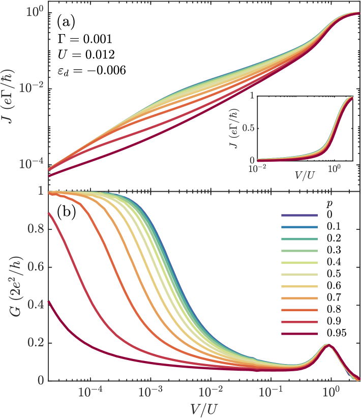
The mean current and the corresponding differential conductance through the system calculated at the particle-hole symmetry point () for different values of the lead spin polarization are presented in Fig. 2. For this we always evaluate the symmetrized current as discussed in App. A.2 [cf. Eq. (14)]. For , we observe a zero-bias conductance peak, characteristic of the Kondo effect [6, 7]. However when is finite, the Kondo temperature is found to decrease with increasing the lead spin polarization. This was predicted to affect the Kondo temperature of the system at equilibrium by using the poor man’s scaling method as [8]
| (10) |
The decrease of the Kondo energy scale with spin polarization can be understood by realizing that by construction with Eq. (5), increasing polarization reduces the hybridization of the suppressed spin orientation. As such, this decreases the rate of spin-flip cotunneling processes responsible for the Kondo effect.
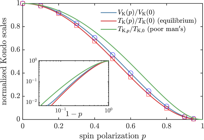
To quantitatively elucidate the influence of on the Kondo effect, we define the Kondo energy scale in the applied bias voltage as the half maxima point of the conductance curve, i.e., at . In Fig. 3 we present the dependence of obtained from our NRG-tDMRG numerical calculations along with the Kondo temperature estimated from Eq. (10) by using the poor man’s scaling, and calculated using the equilibrium NRG [32] from the temperature dependence of the linear conductance based on the definition . Our nonequilibrium data corroborates the general tendency to decrease the Kondo energy scale with increasing the spin polarization . However, Fig. 3 also demonstrates some deviations: is slightly larger than the equilibrium , but smaller than the Kondo temperature predicted by the analytical formula (10), after normalizing the Kondo energy scales with respect to their respective values at .
III.2 Effect of finite exchange field
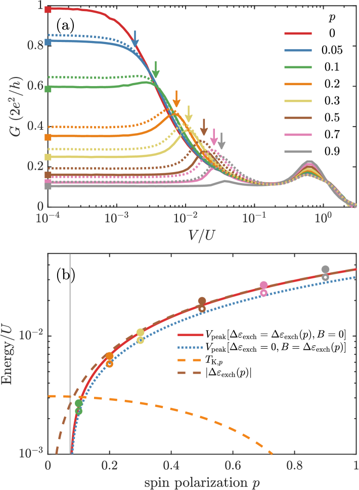
We now discuss the behavior of the differential conductance in the case when the energy level is away from the p-h symmetry point (), but still in the local moment regime where the strong electron correlations play a vital role. The solid lines in Figure 4(a) show the bias dependence of the conductance with increase in the lead spin polarization , computed at zero external magnetic field. One observes a finite zero-bias peak that gets suppressed when grows. This effect can be attributed to the emergence of exchange field in the system, cf. Eq (8). The exchange field introduces a spin splitting of the orbital level, which suppresses the Kondo resonance, once . The color-coded arrows in Fig. 4(a) indicate the magnitude of the exchange field for the corresponding spin polarizations obtained from Eq. (8) with . When the exchange field energy approaches the Kondo energy scale of the system, , the zero-bias conductance becomes suppressed. When increasing the spin polarization further, the differential conductance starts to develop a peak around , which is a reminiscent of the splitting of the local density of states (lDOS) vs. frequency in the presence of a sufficiently strong local magnetic field. To be specific, the peak in the differential conductance presented in Fig. 4(a) emerges for . For this value of spin polarization, one can find that . Increasing the polarization further, the peak at persists while at the same time, the conductance overall also diminishes.
The dotted lines in Fig. 4(a) correspond to the case in which the system has no exchange field (i.e., ), but there is an external magnetic field applied, whose magnitude equals the exchange field calculated from Eq. (8) according to the spin polarizations mentioned in Fig. 4(a). This comparison shows two major differences between the exchange field and the magnetic field. Firstly, a strong enough exchange field suppresses the split-Kondo peak in the differential conductance significantly more strongly and only leaves a residual conductance derived from the hybridization side peaks energies [note the log-scale in Fig. 4 (a)]. This is mainly attributed to the fact that the Kondo scale gets reduced with increasing the spin polarization [cf. Fig. 3], such that the ratio is enhanced for the presence of an exchange field when compared to a local magnetic field. Secondly, the location of the split Kondo peak for finite occurs at slightly higher voltages than for the case of a local magnetic field. The latter effect may be attributed to representing a lowest-order estimate. The explicit dependence of on the spin polarization in the two above-discussed cases is shown in Fig. 4(b). For comparison, we also present the -dependence of and estimated from the respective analytical formulas. One can see that indeed the split Kondo peak emerges when . Moreover, by comparing and , one can find that these two energy scales become equal for . Keeping in mind that this is an approximate estimate, our numerical results corroborate this tendency very well. The split-Kondo peak shows a slightly nonlinear behavior around low spin polarizations. We fit the data against to unveil any behavior of the form . Both the fits for the exchange field and the corresponding magnetic field give essentially the same value of indicated by the grey vertical line on panel Fig. 4(b). The prefactor of the fit is exactly one () within numerical accuracy in the presence of polarization, having [cf. Eq. (9)]. This is also clearly seen in Fig. 4(b) in that the fit exactly coincides with for larger . In the case of a substitute local magnetic field but unpolarized leads, the fit reads . This systematically offsets the peaks with the dashed data in Fig. 4(a) by a constant factor towards slightly smaller values of the bias voltage, yet leads to a disappearance of the split-peak at around the same polarization . On the semilog scale in Fig. 4(b) this change in the prefactor simply shifts the fits vertically relative to each other as also reflected in the data for the full polarization range.
The symbols on the left vertical axis in Fig. 4(a) correspond to the linear response data obtained by NRG, which is equivalent to the differential conductance for . As also seen in later figures, while we have good overall consistency [e.g., see inset of Fig. 6(b)], there are minor quantitative differences in the NRG-tDMRG results while comparing with the linear-response NRG results. These are attributed to the different parametrization and discretization schemes. Specifically, linear conductance within linear response in NRG can be obtained strictly at [33]. In constrast, the NRG-tDMRG approach always must assume a small but finite voltage in the presence of a finite level spacing with the objective to numerically compute a steady-state current via a real-time simulation.
III.3 The influence of magnetic field
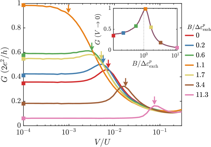
In Fig. 5 we study the influence of external magnetic field on the split Kondo peak exhibited by the system detuned out of the p-h symmetry point assuming the lead spin polarization . We observe a full restoration of the zero-bias Kondo resonance by an applied magnetic field with magnitude that can counterbalance the spin splitting induced by the exchange field, see the curve for in Fig. 5. However, a further increase in magnetic field is shown to suppress the zero-bias peak again. This behavior qualitatively matches the experimental results discussed in the Fig. 2 of the Ref. [14]. As seen from the color-coded arrows in Fig. 5, the position of the split Kondo resonance corresponds to as defined in Eq. (7). The revival of the Kondo resonance can be distinctly observed from the inset of Fig. 5 where exhibits a maximum around such that [Eq. (7)]. More precisely, from in the inset of Fig. 5, , with the small difference primarily attributed to the perturbative nature of the analytic formula Eq. (8). The prefactor approximately coincides with a similar scale factor already encountered with Fig. 4(b) where also underestimated the peak position by an approximate factor .
III.4 Temperature dependence of split Kondo peak
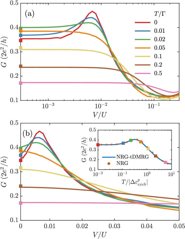
In this section we analyze the effect of finite temperature on the split Kondo resonance. Figure 6 shows the bias voltage dependence of the differential conductance for various temperatures calculated for and . One can see that increasing results in the suppression of the split Kondo peak, which completely disappears once the thermal energy exceeds the induced exchange splitting. Increasing temperature still further overall suppresses the differential conductance. The suppression of the split-Kondo peak is accompanied with a weak increase of the conductance at zero bias for temperatures corresponding to the splitting of the lDOS due to the exchange field, as seen in the inset of Fig. 6(b). This can be used to estimate the temperature where the splitting in the differential conductance disappears. The split-Kondo peak can survive up to a maximum temperature defined as the temperature in which . For the spin polarization , we estimate .
The differential conductance is equivalent to linear-response in thermal equilibrium. The latter is readily obtained by NRG, with a direct comparison shown in the inset of Fig. 6(b). Overall, we observe good quantitative agreement. The points corresponding to the temperatures plotted in the main panels are marked by the same color-matched symbols (squares). Since linear response can be efficiently obtained by NRG, this permits a more dense set of data points in the inset.
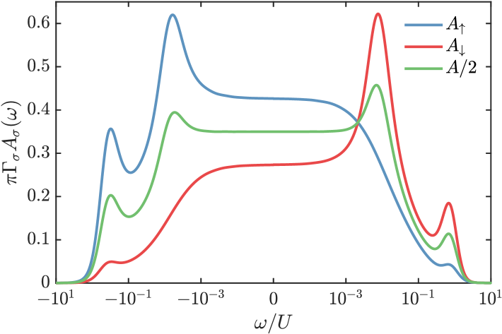
The weak increase in the linear-response conductance for a finite temperature can be explained by examining the energy dependence of the equilibrium local density of states, i.e., the impurity spectral function, assuming that this lDOS changes only weakly at low temperatures . The linear-response conductance is obtained from the spectral function using [33], where is the spin-resolved spectral function based on the retarded impurity Green’s function , and is the derivative of the Fermi function at temperature . Now if the exchange field due to polarization is sufficiently strong, , this will already split the spin-averaged lDOS at equilibrium, as shown for in Fig. 7. When temperature is increased, the transport window widens, and thus encompasses more weight from the split peaks. Assuming that the lDOS only changes weakly by turning on a small temperature , the contributions from the peak in the spectral function around will therefore increase the linear-response conductance up to , where it reaches a maximum before it starts to decrease.
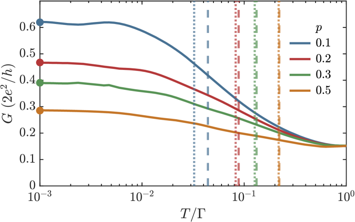
An explicit temperature dependence of the split-Kondo peak conductance for a few selected values of spin polarization is shown in Fig. 8. This figure is determined at finite bias voltage , i.e. at the voltage corresponding to the location of the split Kondo peak shown in Fig. 4. As seen by the vertical markers in Fig. 8, agrees well with for large polarization , but clearly starts to differ for smaller , given that there is no peak at finite for . By starting from the peak conductance, one can now clearly see in Fig. 8 the decrease of the remaining side Kondo resonance as the temperature increases. The logarithmic decrease in the split-Kondo peak conductance at higher temperatures has been experimentally observed in the Fig. 3a of Ref.[9]. In the case of , the split Kondo peak just emerged, having , as can be observed from Fig. 4 and the vertical blue lines in Fig. 8. Hence, we can see a slight non-monotonic behavior arising from the interplay between the Kondo effect and the exchange field. More generally, one can infer from Figs. 6 and 8, for the split-Kondo regime, i.e., sufficiently strong polarization with , that vs. [ vs. ] will exhibit a non-monotonic behavior if [], yet a monotonic decay if [or ], respectively. We also note that the temperature dependence of the non-equilibrium differential conductance at does not show a universal dependence. This can be understood by realizing that the system is then out of the Kondo regime.
IV Summary
In this paper we have studied the non-equilibrium spin-resolved transport through a quantum dot coupled to ferromagnetic leads, while treating the correlations exactly. When the dot level is at the particle-hole symmetry point, we have shown that the Kondo resonance can be observed for any value of spin polarization , but the Kondo energy scale in the bias potential reduces with increasing spin polarization. However, when the dot level is detuned out of the particle-hole symmetry point, we have observed the emergence of an exchange field in the system, which splits the zero-bias conductance peak when it is comparable or larger than the Kondo energy scale. A finite value of magnetic field was able to restore the Kondo resonance in such system. Moreover, we have determined the temperature dependence of the split Kondo peak and showed that the character of this dependence depends on the ratio of exchange field to the Kondo energy scale. Our work provides benchmark results for the nonequilibrium spintronic transport through quantum impurity systems in the presence of ferromagnetic leads.
Acknowledgements.
This work was supported by the Polish National Science Centre from funds awarded through the decision Nos. 2017/27/B/ST3/00621 and 2021/41/N/ST3/02098. We would also like to acknowledge the support by the project “Initiative of Excellence - Research University” from funds awarded through Decision no: 003/13/UAM/0016. AW was supported by the U.S. Department of Energy (DOE) Office of Basic Energy Sciences (BES), Materials Sciences and Engineering Devision.Appendix A The hybrid NRG-tDMRG thermofield quench approach
This appendix provides more details on the hybrid NRG-tDMRG thermofield quench method [29] used to calculate the spin-resolved transport properties of the system in non-equilibrium settings.
A.1 Thermofield treatment of the leads
To describe the leads we use the thermofield approach [34, 35, 30], in which an auxiliary Hilbert space, equivalent to the lead Hilbert space, but decoupled from the system, is introduced to the lead Hamiltonian, effectively doubling the Hilbert space. This allows us to simplify the computational problem, since the decoupled modes of thermal leads can be expressed as simple product states. More importantly, thermofield approach enables the description of the thermal states as pure states, which can be then time-evolved within the matrix product state framework.
A pure state is defined on this enlarged space such that the thermal expectation value of an observable in the original physical Hilbert space can be obtained from the enlarged space using , where the state is defined as
| (11) |
Here, the composite index corresponds to , , and the Fock states, and , which act as the basis for the new Hilbert space, are defined as, . We define the modes in a rotated basis such that, , using the transformation,
| (12) |
With this transformation, the initial pure product state is such that , which essentially results in one set of modes () to be fully occupied, while the rest () is empty. The fully filled (empty) states in the new basis resemble the particle (hole) description of the lead Hamiltonian. The particles and holes will be recombined later for the NRG part of the calculations but treated separately for the tDMRG time evolution as described later.
A.2 The hybrid NRG-tDMRG time evolution
The hybrid NRG-tDMRG approach we employ combines the strong assets of both NRG and DMRG, namely, the ability of NRG to resolve logarithmic energy scales and the ability of DMRG to describe nonequilibrium situations at energy scales close to the bandwidth. One fundamental difference between the both methods is that while NRG is fundamentally based on logarithmic discretization, DMRG studies have found incredible success based on a linear discretization of the lead energy continuum. The energy scales that distinguish the regimes of implementation of these methods are denoted by the transport window (TW), which is determined by a difference in the electrochemical potentials of the leads, . Assuming that the lead levels far from the TW are essentially in equilibrium, we implement a logarithmic discretization scheme outside the transport window in order to later treat them with the aid of the NRG. On the other hand, the energies inside the TW are discretized linearly to be compatible with the DMRG formalism. The discretized energy intervals are denoted by and defined as,
where and are the linear and logarithmic discretization parameters, respectively. The energy levels outside the TW are treated using the numerical renormalization group method, giving rise to a renormalized impurity (RI) with a reduced effective bandwidth . As a result of the thermofield transformation in the linear sector, the system can be effectively described as renormalized impurity coupled to two chains, corresponding to the tridiagonalized chains of the particle and hole modes.
The Hamiltonians, and , transform according to the aforementioned rotation as,
| (13) |
where and the transformed couplings and . After the transformation, we recombine the particles and holes in the logarithmically discretized regime through another tridiagonalization in order to apply NRG. Furthermore, we recombine the transformed left and right lead modes so that one set of modes decouples from the system, as is common in the case of equilibrium NRG studies [27].
We perform a second order Trotter time evolution on the initial state of the system, , during which the coupling between the linear and logarithmic sectors is switched on over a finite time interval. Here, is the initial state of the RI and is the pure product state of the linear sector. We calculate the symmetrized current
| (14) |
at each time step of the system’s evolution, where () is defined as the current flowing from the left (right) lead to the impurity and . The system is time-evolved until the relevant observables start to fluctuate around a mean value and a nonequilibrium steady state is reached. We evaluate our main quantity of interest—the current—as the mean of the symmetrized current over a finite time interval where the system shows steady state behavior. The averaging time window is chosen by scanning through the current dynamics to find the one with least error around the mean value. The corresponding differential conductance is calculated from the mean symmetrized current. Both NRG and tDMRG calculations are implemented in the matrix product state framework [36]. In calculations we assume and .
References
- Žutić et al. [2004] I. Žutić, J. Fabian, and S. Das Sarma, Spintronics: Fundamentals and applications, Rev. Mod. Phys. 76, 323 (2004).
- Bauer et al. [2012] G. E. W. Bauer, E. Saitoh, and B. J. van Wees, Spin caloritronics - Nature Materials, Nat. Mater. 11, 391 (2012).
- Awschalom et al. [2013] D. D. Awschalom, L. C. Bassett, A. S. Dzurak, E. L. Hu, and J. R. Petta, Quantum Spintronics: Engineering and Manipulating Atom-Like Spins in Semiconductors, Science 339, 1174 (2013).
- Hirohata et al. [2020] A. Hirohata, K. Yamada, Y. Nakatani, I.-L. Prejbeanu, B. Diény, P. Pirro, and B. Hillebrands, Review on spintronics: Principles and device applications, J. Magn. Magn. Mater. 509, 166711 (2020).
- Hewson [1993] A. C. Hewson, The Kondo Problem to Heavy Fermions, Cambridge Studies in Magnetism (Cambridge University Press, 1993).
- Goldhaber-Gordon et al. [1998] D. Goldhaber-Gordon, H. Shtrikman, D. Mahalu, D. Abusch-Magder, U. Meirav, and M. A. Kastner, Kondo effect in a single-electron transistor, Nature 391, 156 (1998).
- Cronenwett et al. [1998] S. M. Cronenwett, T. H. Oosterkamp, and L. P. Kouwenhoven, A Tunable Kondo Effect in Quantum Dots, Science 281, 540 (1998).
- Martinek et al. [2003a] J. Martinek, Y. Utsumi, H. Imamura, J. Barnaś, S. Maekawa, J. König, and G. Schön, Kondo Effect in Quantum Dots Coupled to Ferromagnetic Leads, Phys. Rev. Lett. 91, 127203 (2003a).
- Pasupathy et al. [2004] A. N. Pasupathy, R. C. Bialczak, J. Martinek, J. E. Grose, L. A. K. Donev, P. L. McEuen, and D. C. Ralph, The Kondo Effect in the Presence of Ferromagnetism, Science 306, 86 (2004).
- Yazdani et al. [1997] A. Yazdani, B. A. Jones, C. P. Lutz, M. F. Crommie, and D. M. Eigler, Probing the Local Effects of Magnetic Impurities on Superconductivity, Science 275, 1767 (1997).
- Franke et al. [2011] K. J. Franke, G. Schulze, and J. I. Pascual, Competition of Superconducting Phenomena and Kondo Screening at the Nanoscale, Science 332, 940 (2011).
- Seneor et al. [2007] P. Seneor, A. Bernand-Mantel, and F. Petroff, Nanospintronics: when spintronics meets single electron physics, J. Phys.: Condens. Matter 19, 165222 (2007).
- Barnaś and Weymann [2008] J. Barnaś and I. Weymann, Spin effects in single-electron tunnelling, Journal of Physics: Condensed Matter 20, 423202 (2008).
- Hamaya et al. [2007] K. Hamaya, M. Kitabatake, K. Shibata, M. Jung, M. Kawamura, K. Hirakawa, T. Machida, T. Taniyama, S. Ishida, and Y. Arakawa, Kondo effect in a semiconductor quantum dot coupled to ferromagnetic electrodes, Appl. Phys. Lett. 91, 232105 (2007).
- Hauptmann et al. [2008] J. R. Hauptmann, J. Paaske, and P. E. Lindelof, Electric-field-controlled spin reversal in a quantum dot with ferromagnetic contacts, Nat. Phys. 4, 373 (2008).
- Gaass et al. [2011] M. Gaass, A. K. Hüttel, K. Kang, I. Weymann, J. von Delft, and Ch. Strunk, Universality of the Kondo Effect in Quantum Dots with Ferromagnetic Leads, Phys. Rev. Lett. 107, 176808 (2011).
- Martinek et al. [2003b] J. Martinek, M. Sindel, L. Borda, J. Barnaś, J. König, G. Schön, and J. von Delft, Kondo Effect in the Presence of Itinerant-Electron Ferromagnetism Studied with the Numerical Renormalization Group Method, Phys. Rev. Lett. 91, 247202 (2003b).
- López and Sánchez [2003] R. López and D. Sánchez, Nonequilibrium Spintronic Transport through an Artificial Kondo Impurity: Conductance, Magnetoresistance, and Shot Noise, Phys. Rev. Lett. 90, 116602 (2003).
- Utsumi et al. [2005] Y. Utsumi, J. Martinek, G. Schön, H. Imamura, and S. Maekawa, Nonequilibrium Kondo effect in a quantum dot coupled to ferromagnetic leads, Phys. Rev. B 71, 245116 (2005).
- Świrkowicz et al. [2006] R. Świrkowicz, M. Wilczyński, M. Wawrzyniak, and J. Barnaś, Kondo effect in quantum dots coupled to ferromagnetic leads with noncollinear magnetizations, Phys. Rev. B 73, 193312 (2006).
- Weymann and Borda [2010] I. Weymann and L. Borda, Underscreened Kondo effect in quantum dots coupled to ferromagnetic leads, Phys. Rev. B 81, 115445 (2010).
- Žitko et al. [2012] R. Žitko, J. S. Lim, R. López, J. Martinek, and P. Simon, Tunable Kondo Effect in a Double Quantum Dot Coupled to Ferromagnetic Contacts, Phys. Rev. Lett. 108, 166605 (2012).
- Wójcik and Weymann [2015] K. P. Wójcik and I. Weymann, Two-stage Kondo effect in T-shaped double quantum dots with ferromagnetic leads, Phys. Rev. B 91, 134422 (2015).
- Weymann et al. [2018] I. Weymann, R. Chirla, P. Trocha, and C. P. Moca, SU(4) Kondo effect in double quantum dots with ferromagnetic leads, Phys. Rev. B 97, 085404 (2018).
- Bordoloi et al. [2020] A. Bordoloi, V. Zannier, L. Sorba, C. Schönenberger, and A. Baumgartner, A double quantum dot spin valve, Commun. Phys. 3, 1 (2020).
- Wilson [1975] K. G. Wilson, The renormalization group: Critical phenomena and the Kondo problem, Rev. Mod. Phys. 47, 773 (1975).
- Bulla et al. [2008] R. Bulla, T. A. Costi, and T. Pruschke, Numerical renormalization group method for quantum impurity systems, Rev. Mod. Phys. 80, 395 (2008).
- Schollwöck [2011] U. Schollwöck, The density-matrix renormalization group in the age of matrix product states, Annals of Physics 326, 96 (2011), january 2011 Special Issue.
- Schwarz et al. [2018] F. Schwarz, I. Weymann, J. von Delft, and A. Weichselbaum, Nonequilibrium Steady-State Transport in Quantum Impurity Models: A Thermofield and Quantum Quench Approach Using Matrix Product States, Phys. Rev. Lett. 121, 137702 (2018).
- de Vega and Bañuls [2015] I. de Vega and M.-C. Bañuls, Thermofield-based chain-mapping approach for open quantum systems, Phys. Rev. A 92, 052116 (2015).
- Anderson [1961] P. W. Anderson, Localized Magnetic States in Metals, Phys. Rev. 124, 41 (1961).
- [32] We used the open-access Budapest Flexible DM-NRG code, http://www.phy.bme.hu/˜dmnrg/; O. Legeza, C. P. Moca, A. I. Tóth, I. Weymann, G. Zaránd, arXiv:0809.3143 (2008) (unpublished) .
- Meir et al. [1991] Y. Meir, N. S. Wingreen, and P. A. Lee, Transport through a strongly interacting electron system: Theory of periodic conductance oscillations, Phys. Rev. Lett. 66, 3048 (1991).
- Barnett and Dalton [1987] S. M. Barnett and B. J. Dalton, Liouville space description of thermofields and their generalisations, J. Phys. A: Math. Gen. 20, 411 (1987).
- Das [2000] A. Das, Topics in Finite Temperature Field Theory, ArXiv (2000), hep-ph/0004125 .
- Weichselbaum [2012] A. Weichselbaum, Tensor networks and the numerical renormalization group, Phys. Rev. B 86, 245124 (2012).