Nonequilibrium Steady States for Certain
Hamiltonian Models
Abstract
We report the results of a numerical study of nonequilibrium steady states for a class of Hamiltonian models. In these models of coupled matter-energy transport, particles exchange energy through collisions with pinned-down rotating disks. In [16], Eckmann and Young studied 1D chains and showed that certain simple formulas give excellent approximations of energy and particle density profiles. Keeping the basic mode of interaction in [16], we extend their prediction scheme to a number of new settings: 2D systems on different lattices, driven by a variety of boundary (heat bath) conditions including the use of thermostats. Particle-conserving models of the same type are shown to behave similarly. The second half of this paper examines memory and finite-size effects, which appear to impact only minimally the profiles of the models tested in [16]. We demonstrate that these effects can be significant or insignificant depending on the local geometry. Dynamical mechanisms are proposed, and in the case of directional bias in particle trajectories due to memory, correction schemes are derived and shown to give accurate predictions.
Introduction
Explaining far-from-equilibrium macroscopic phenomena on the basis of microscopic dynamical mechanisms is one of the basic problems of nonequilibrium statistical mechanics. This paper presents the results of some numerical studies aimed at shedding light on “micro-to-macro” questions for a class of mechanical models introduced in [35, 27, 16] as paradigms for transport processes. Here as in [16], the basic idea is that macroscopic quantities such as energy and density profiles can be deduced – easily and fairly accurately – from certain information on local dynamics provided one makes a couple of simplifying assumptions. In this paper, we extend the results in [16] to a larger class of models and at the same time examine more closely the extent to which these assumptions hold. These questions lead to a systematic study of how geometry impacts memory and finite-size effects.
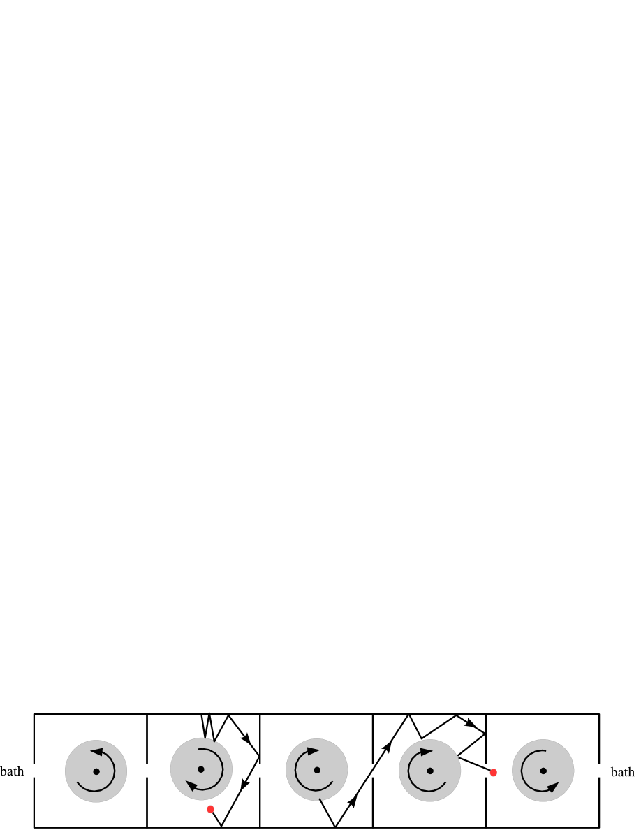
The models studied in this paper describe a coupled transport of matter and energy. The local dynamics are purely deterministic and energy-conserving; that is what we mean by “Hamiltonian” in this paper. The system is attached to (unequal) stochastic heat baths which both inject particles into the system and absorb those that leave. Placed throughout the system, evenly spaced, are rotating disks that are nailed down at their centers; particles exchange energy with them upon collisions. This interaction was first used in [35] and [27]; it takes the place of direct particle-particle interactions, which are more delicate to control. The authors of [16] introduced the following conceptual simplification: each rotating disk is enclosed in a well-defined area called a cell, with small enough passageways between cells to ensure equilibration within each cell. Motivated by this “decoupling” of internal cell dynamics and cell-to-cell traffic, they proposed a scheme that yields simple explicit expressions for approximate energy profiles and particle densities. The scheme is based on two assumptions: that cell-to-cell movement takes essentially the form of an unbiased random walk, and that within each cell, the system attains local thermal equilibrium quickly. They found striking agreement between their proposed formulas and simulation results, with barely visible errors for chains consisting of no more than 30 cells.
The aims of this paper are twofold. One is a straightforward extension of the results in [16] to a larger class of models. Keeping the basic interaction as well as cell structure in the last paragraph, we have found the prediction scheme in [16] – suitably modified – to be very flexible. To give a sense of the type of generalizations, our simulations are in 2D, but we expect similar results to hold in 3D (with rotating balls in the place of rotating disks). In dimensions greater than one, there are different choices of lattices and boundary conditions. We show that this scheme is equally valid for rectangular and hexagonal lattices, and for all of the boundary conditions tested. The resulting profiles are, of course, different in each case. We permit even point sources and the use of thermostats to regulate temperature in different parts of the domain. These and other features are illustrated in Examples 1–3 in Sect. 2. We also extend the results in [16] in a different direction, to “closed” systems, i.e., systems in which the total particle number is conserved and system-bath interactions are limited to energy exchange (Sect. 4).
Our second aim is to understand why memory and finite-size effects are so mild in the models tested, or, put differently, why a scheme that ignores these effects can perform so well in profile predictions. Here we find the key to lie in cell geometry, referring roughly to the geometric relation of cell walls and passageways to the rotating disk. To examine these issues in greater depth, we consider a broader class of cell designs. Among the geometries studied here, the one that represents the greatest departure from the ideas in [16] (see above) is used in Examples 5 and 6(A) in Sect. 3.3 (respectively Figs. 9(a) and 10(a)). In these examples, walls between cells are broken down altogether leaving a domain with rotating disks inside. To summarize, we find that finite-size and memory effects can be significant or insignificant. By understanding the dynamical mechanisms behind them, we learn to identify “good” and “bad” geometries. With regard to directional bias in particle trajectories due to memory, an issue also addressed in [15], in Sect. 3.1 we offer a correction scheme that is proven to be effective for systems with “bad geometry.”
Stochastic idealizations. Alongside the Hamiltonian models, the authors of [16] introduced a class of Markov jump processes intended to be their stochastic idealizations. Our generalizations in Sects. 2 and 4 apply also to these stochastic models. We have run many tests, and have found – without exception – that the simulations converge easily to predicted values (with, not surprisingly, smaller errors and faster convergence rates than for their Hamiltonian counterparts). While this class of stochastic models, sometimes called “random-halves models” (see [32]), are interesting in their own right, we have elected to focus on Hamiltonian models in this paper because they are both more complex and more physical.
Related works. For reviews of some general physical and mathematical issues involved in the study of nonequilibrium steady states and transport processes, see, e.g., [6, 19, 22, 29, 40, 41, 44]. Much more is known in the context of stochastic models or models with a significant stochastic component. Of the considerable literature on that topic, we cite here a few that are most closely related to the present study: [2, 3, 4, 5, 11, 12, 25, 26, 30, 32, 34, 36]. The literature on models with purely deterministic internal dynamics is more sparse. In addition to the articles already cited, [1, 7, 9, 10, 13, 14, 21, 23, 31, 37, 38, 42] are the main ones we know of. Finally, aside from putting [16] in the more general contexts to which it belongs, we have taken some small steps in this paper to connect geometry and local dynamics to nonequilibrium properties, a connection that, in general, remains to be understood.
1 Review of models and results in [16]
Since the present paper is an extension of [16] with a focus on Hamiltonian models, we begin with a brief review of the models and relevant findings in the Hamiltonian part of [16].
1.1 Description of models
Single cell in isolation. Let be a bounded, simply connected planar region with piecewise- boundary. A disk is placed in the interior of ; its center is fixed, and it is allowed to rotate freely about its center. The state of the disk is given by , where is the angle (relative to a marked reference point) and its angular velocity. A number of particles move about in the cell. The state of a particle is given by , where is its position and its velocity. Particles fly freely with constant velocity until they hit either or (they do not interact with each other directly). A particle that collides with reflects elastically:
where is the collision time, is the component of the particle’s velocity tangential to , and is the normal component. When a particle hits , the particle swaps its tangential velocity with the disk’s angular velocity:
We assume that the masses of the particles and the moment of inertia of the rotating disk are scaled so that the kinetic energy of each particle is and the rotational energy of the disk is . Energy is conserved in the interaction rule above.
Single cell coupled to two heat baths. Suppose now the cell has two openings, which we identify with subsets . It is useful (though not necessary) to think of as having a left-right symmetry, and and as symmetrically placed on the left and right sides of respectively. These two openings are connected to two heat baths that absorb and emit particles. A particle absorbed by one of the baths leaves the system forever. Each bath is characterized by two parameters, a temperature and an injection rate . A Poisson clock of rate is associated with each bath. When its clock rings, the bath places a new particle into the system at a (uniformly) random position , where for the left bath and for the right bath. The particle is assigned a random (I.I.D.) velocity sampled from the distribution
| (1) |
where and is the angle between and , measured so that points into . The actions of the two baths are independent.
1D-chain coupled to two heat baths. Consider copies of the cell described above – call them – each with two openings and symmetrically placed. We think of these cells as occupying integer sites , and for each identify the right opening of the th cell with the left opening of the st cell, so that particles are able to pass from cell to cell along the chain. Sites and are occupied by heat baths which inject particles into (and absorb particles from) cells and respectively. The rules of injection are as above.
Remarks. (i) We note that except for the chain-bath interaction, which is stochastic in nature, the dynamics within the chain are purely deterministic and energy-conserving. It is for this reason that we refer to these models as Hamiltonian chains. The local dynamics are, in fact, not symplectic at collisions between particles and rotating disks. (ii) Even though particles do not interact directly with each other, they do interact quite strongly via the disks, and the overall character of the dynamics is very strongly nonlinear.
Equilibrium distributions. The following result characterizes the Hamiltonian chain in thermal equilibrium with two equal heat baths.
Theorem 1 (Eckmann-Young [16]).
Consider an -chain in contact with two baths, both with temperature and rate :
-
1.
Single cells. For , the system preserves a probability measure characterized by the following properties: The number of particles in the cell is a Poisson random variable with mean
where is the length of an opening. The conditional measure of on , the state space for a single cell containing indistinguishable particles, is given by
where and is the normalizing constant.
-
2.
-chains. Let , , be copies of . An -chain in contact with two equal baths held at preserves the product measure .
Here are a few different ways to measure temperature for a cell with distribution :
-
1.
The mean disk energy, , is .
-
2.
The mean energy per particle in the cell, , is .
-
3.
The expected energy of a particle exiting the cell is ; its distribution is given by Eq. (1).
Nonequilibrium steady states. Suppose a chain is connected to two unequal heat baths, i.e., , where and are the temperatures of the left and right heat baths respectively, and and are their respective injection rates. It was found numerically in [16] (though not proved) that irrespective of initial condition, following a transient the system settles down to a nonequilibrium steady state determined solely by the quadruple . The product nature of the equilibrium distribution in Theorem 1 depends crucially on having detailed balance within the system (see [16]). In nonequilibrium steady states, there is no longer detailed balance, and the invariant measure cannot be explicitly computed. In particular, the system has spatial correlations, and the steady state distribution is not of product form.
1.2 Scheme for predicting nonequilibrium profiles proposed in [16]
In this subsection we review the scheme proposed in [16] for deducing approximate mean disk energies, temperatures, and other profiles in chains that are out of equilibrium. This scheme is based on the following ideas:
Assumption 1. The system is close to having zero directional bias. When a particle leaves a cell, let denote the probability that it exits to the left and the probability that it exits to the right. By zero bias, we mean , regardless of the state of the particle at the time it entered the cell or the state of the cell while it is there.
Assumption 2. The system is close to local equilibrium. Given , , , and (with ) and , let denote the marginal distribution of the invariant measure for an -chain at site . We assume there are numbers and independent of such that for the -chain in question, is close to where is as in Sect. 2.1.
The rationale for the first assumption is that when the length of the opening is small, a particle will remain inside each cell it visits for a long time, eventually losing memory of past events. The second assumption is based on the idea of local thermal equilibrium (LTE) [22, 25], which, if true for these models, will imply the convergence of to as . The idea in [16] is to treat the approximations in Assumptions 1 and 2 as though they were exact, and to derive under these simplifying assumptions mean energy and particle density profiles.
Derivation of profiles assuming zero bias and local equilibrium. All means below are taken at steady state. For each cell , let
By , we refer here to the total number of particles exiting cell via either one of its two exits, and similarly for . Taking the approximation in Assumption 1 to be exact, we get, from the conservation of mass and energy,
with boundary conditions
It follows that the quantities and linearly interpolate between the boundary conditions. As , and converge (trivially) to
for all . Returning to the -chain, the local equilibrium assumption together with Theorem 1 then tells us that for cell , we have , leading to the
(We think of the th cell as occupying location and the baths as located at .) Similarly, we find the
Additional profiles, e.g., total kinetic energy in each cell, are also easily deduced.
Remarks. Mathematically, that the formulas above give approximate profiles for sufficiently long chains of cells with sufficiently small openings will follow from the continuity of the observables and in the double limit of zero-bias and infinite volume, the former to be interpreted as . Such limits are far from trivial. Rigorous results are out of reach at the present time.
In [16], simulations were performed for models in which is given by the area enclosed by four overlapping disks with small openings introduced, and results were reported for 1D-chains with various parameters. It was found that even for relatively small , e.g., , the predictions above compare surprisingly well against empirical data. This suggests that for the models tested, (i) memory effects leading to directional bias in particle movements are indeed negligible, and (ii) local equilibrium is, to a good approximation, achieved at relatively small , i.e., finite size effects are insignificant.
2 Generalization to larger class of models
In this section, we generalize the results of [16] in a variety of directions, including:
-
-
Higher dimensions. We focus on 2D models; phenomena in higher dimensions are expected to be similar.
-
-
Lattice types. In two or more dimensions, there are different lattice types. We focus here on rectangular and hexagonal geometries.
-
-
Boundary conditions. Dirichlet, periodic, and reflecting boundary conditions are considered. We show that our scheme applies even to point sources.
-
-
Thermostats. By this we refer to the use of external means to maintain or regulate the temperature of various parts of the system.
Instead of giving a formal treatment of each of these generalizations, we will present in Sects. 2.1–2.3 below three examples that systematically illustrate the various effects.
General setup and issues. The following are features common to all the models to be presented. We first discuss them so we can focus on the specific points of interest within each example.
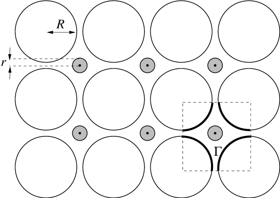
(1) Basic configurations. We start with a lattice of disjoint fixed (non-rotating) disks in . Fig. 2 shows a rectangular array; a hexagonal array is shown in Fig. 5. Particles move in the space between these disks, bouncing off them in specular collisions. The packing is relatively dense, with narrow channels between adjacent disks to allow the passage of particles. The area in between this array of fixed disks is partitioned into identical cells whose walls are circular arcs (pieces of boundaries of the fixed disks) alternating with openings called gaps; see Fig. 2. At the center of each cell is a rotating disk, with which particles exchange energy following the rules in Sect. 1.1. Disk energy will always refer to the kinetic energy of a rotating disk.
(2) Mixing rates and geometry. We use and to denote respectively the radii of the fixed and rotating disks. These two numbers together with the distance between the centers of the fixed disks will affect the number of collisions a particle experiences before it finds its way out of a cell. More collisions will naturally lead to better equilibration within cells. Too many such collisions, on the other hand, will delay mixing on a more global scale and slow down convergence to steady state. Information on the expected number of collisions can be deduced from Theorem 1. For example, on each visit to a cell, the number of collisions between a particle and the rotating disk is, on average, .
(3) Continuum limits. Our domains of interest are bounded. Formally, we fix a region with piecewise smooth boundary, and consider a sequence of homothetically magnified images of . At stage , the fixed disks in the system are those that meet . To obtain continuum limits of profiles for disk energy, particle counts, etc., we map back to (so that the profiles for different are all defined on ) and take .
(4) Predicted vs. simulated results. In each of the examples below, we will report the percentage discrepancy between the predicted and simulated values of energy, particle count, etc. Our predictions are based on exact versions of the two assumptions in Sect. 1.2, which cannot be true for finite chains with finite gap sizes, and the simulated values given are computed empirically for finite – and only moderately large – systems.
Remark on numerical simulations. All numerical results in this paper are computed by direct Monte Carlo computations, i.e., expectations are estimated by ergodic averages based on long-time simulations. We prepare the system by sampling the equilibrium distribution at a uniform temperature , where is usually chosen to be the maximum of the boundary temperatures, and evolve the system for events (an event is a single particle-disk collision, bath injection, or particle exit). Statistical errors are quantified by a standard batch means method. Typical relative errors for the simulations in this section are . For example, for the results in Fig. 3 below, the (absolute) standard error for the profile is estimated to be and the relative error is at the 95% confidence level.
2.1 Example 1. Rectangular lattice, Dirichlet boundary conditions
Our first example is a 2D rectangular array on a rectangular-shaped domain with Dirichlet boundary conditions (to be explained). Fixed disks of radius are placed at even lattice points We think of as being close to , so that each square configuration of 4 fixed disks bounds an open cell with 4 narrow gaps, with gap size . In the center of each cell, i.e., at odd lattice points , we place a small rotating disk of radius . Heat baths are viewed as occupying the strip of cells just outside the system, injecting and removing particles through the associated openings. For simplicity, we consider only configurations where all baths along the same edge have the same parameters . For example, if the bath along the left edge has parameters , then particles with energies distributed according to Eq. (1) with are injected at rate into each cell in the leftmost column, through its opening on the left. We refer to the boundary condition described above as a “Dirichlet” boundary condition.
Profile prediction. The scheme reviewed in Sect. 1.2 is easily generalized to the present setting. Formulating Assumption 1 in 2D is straightforward: it is equivalent to requiring that the probability of exiting any of the 4 openings to be . The precise meaning of LTE here is as follows: let be the fixed domain on which the continuum limit will be taken, and set and for positive integers . Then for every , the marginal distribution of the cell at site tends to for some and as .
Returning to the finite system described in the first paragraph, let and denote the particle and energy exit rate from the th cell. The particle balance equation is the discrete Laplace equation
with boundary conditions on the left edge, on the right edge, etc. The are described by the discrete Laplace equation as well, with boundary conditions on the left, on the right, and so on. In the continuum limit, these equations tend to the Laplace equation with the given boundary values. Solutions for and are then used to compute the mean disk energy and mean particle count through
These formulas are virtually identical to those for 1D-chains given in Sect. 1.2, differing only in some constants, and can be deduced the same way. The differences in constants are due to the fact that each cell here is in contact with 4 (rather than 2) cells/baths.
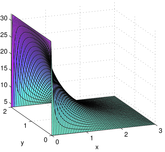
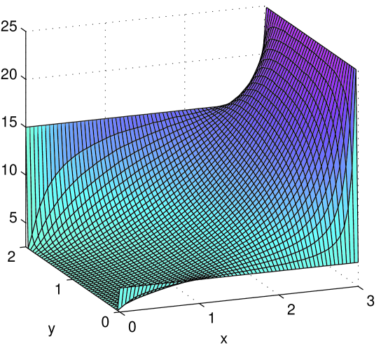
Simulation results. We now compare the predicted profiles to the results of direct simulations. Fig. 3 shows some simulation results using the following boundary conditions:
| cells | ||
Fixed disks have radius and rotating disks . These numbers ensure that on average, each particle experiences collisions and hits the rotating disk times on each pass through a cell.
Fig. 3 shows profiles for the jump rate , the energy exit rate , the mean disk energy , and the particle count . Boundary values have been filled in for ease of visualization. We have found that the discrepancy between simulation results and predicted profiles are greatest in the “L-shaped” regions at corners along the boundary of the domain. Away from these regions, the discrepancy is . That the discrepancy is larger here is clearly due to discontinuous boundary values and finite-size effects.
 |
 |
| (a) | (b) |
 |
 |
| (c) Disk energy | (d) Particle count |
Before leaving this example, let us check our intuition against the plotted profiles. Observe first that panels (a) and (c), i.e., plots of jump rates and disk energies , reflect the boundary conditions in a straightforward way. The saddle-shaped profile of (panel (b)) is also easy to explain: it is because along the 4 edges clockwise from left, has ratios 4 : 3 : 5 : 1 . A factor that influences particle count is that all else being equal, particles tend to gather in low-temperature regions. The reason is that in a steady state, the total particle flux into and out of any region must be equal. At the lower temperature end, particles move slowly, hence more of them are needed to produce the same flux. For the boundary conditions considered here, the accumulation of particles on the left due to colder temperatures is exaggerated by the higher injection rate on the same side. This has resulted in the huge spread for in panel (d), from on the left to on the right. If we change the boundary conditions to , the profile for would be quite a bit flatter. This is both predicted and confirmed in simulations.
Non-Dirichlet boundary conditions. We have obtained similar simulation results for systems with periodic and reflecting boundary conditions in the vertical direction.
2.2 Example 2. System cooled by thermostats
The main novel feature of this example is the use of thermostats in the present context.111See, e.g., [8, 17, 18, 20, 24, 33, 39] for more examples and thorough discussions of thermostats in nonequilibrium statistical mechanics. A second feature of note is the use of exit-only boundaries, which for convenience we will refer to as open boundaries.
Thermostats. For our purposes, a thermostat is a disk with the property that whenever a particle with velocity hits it, the tangential component of the particle’s velocity is instantaneously set to a random value sampled from the distribution
where is the thermostat temperature. The normal component of is updated according to the usual rule: Thus, a particle that hits the thermostated disk sufficiently many times would acquire the energy distribution for temperature . A cell is thermostated if it contains a thermostat in place of a rotating disk.
We consider in this example a cooling system on a finite cylindrical domain with an open boundary at one end. More precisely, the domain is defined by a rectangular array of fixed disks with a periodic boundary condition in the vertical direction. The right end of the cylinder is put in contact with heat baths, with which it has the same type of interaction as in the previous example. The left end of the cylinder has an open boundary, meaning particles can leave but no new particles enter through it. This configuration leads to a particle flux across the system, from right to left. As the relatively hot particles move through the system, they are cooled (either directly or indirectly) by a row of thermostated cells. For simplicity, we assume the thermostated cells occupy exactly one row which extends the full length of the cylinder, and all thermostats in these cells are set to a fixed temperature considerably lower than that of the heat bath.
Profile prediction. To obtain predictions for the various profiles, we proceed as follows:
First, one solves for as before, the only difference being that the boundary conditions for are periodic in the direction. The open boundary for corresponds to setting for all . Solving the boundary value problem readily yields .
To find , the left and right boundaries are treated in a similar fashion as for . To handle thermostats, we assume that the array is mapped to a domain with and identified, and that the thermostats are at . We then set, for each with , , where is as in the last paragraph. This is again a boundary value problem, which can be solved to give .
Once and have been computed, profiles for and are given by the same formulas as in the previous example.
We point out two reasons why one may expect greater discrepancies between predicted and simulated results in the present model than in the Dirichlet case: (1) In setting the “boundary values” for along the row of thermostated cells, we have assumed that the outgoing particles have energy . In reality, a highly-energetic particle that enters a thermostated cell is likely to leave it with somewhat more energy than : it interacts with the rotating disk only a finite number of times, keeping the normal component of its velocity each time. (2) At the open boundary, must necessarily go to zero, as must therefore particle count. Since a healthy number of particles is needed in each cell to ensure proper mixing, the situation near this boundary can be anomalous.
Also, with few particles, a practical concern is inadequate updating during the course of the simulation.
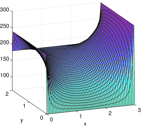
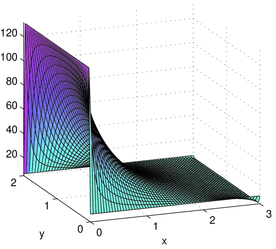
Simulation results. Fig. 4 shows simulation results for the following boundary values:
Again, we use and . Panel (a) shows the mean disk energy , which is higher on the right side due to bath injections and lower along the top and bottom edges due to the cooling effects of the thermostats. Panel (b) shows the particle counts. In addition to the cells near the baths, particles accumulate near the top and bottom boundaries due to the lower temperatures there. Panel (c) compares directly simulation data and predicted values for some cross-sections of the profile, and panel (d) examines the situation along (where the thermostats are) for , i.e., near the bath. As anticipated, the temperature here is higher than its predicted values, with the discrepancy rising sharply as tends to . The particle deficit is then consistent with the fact that exit rates per particle are higher than predicted.
 |
|
| (a) Mean disk energy | (b) Mean particle count |
 |
|
| (c) Slices of at | (d) Slices of and at |
The effects highlighted in panel (d), however, seem confined to the thermostated cells. Away from them, the discrepancy between predicted and simulation profiles are about 1-4% for the mean disk energy and for the particle count. The latter shows larger discrepancies near the open (left) end of the domain, due presumably to near there.
2.3 Example 3. Hexagonal array with point sources
Our third example is a hexagonal array with point sources and open boundaries. The array we use consists of fixed disks of radius placed on the vertices of a triangular mesh; each edge of the mesh has length 1. Each triangular array of 3 fixed disks bounds a cell. At the center of each cell, we place a small rotating disk of radius . See Fig. 5. The system has open boundaries with no bath injections. Instead, it is driven by a finite number of point sources which pump particles directly into the interior of the array. We say a cell contains a point source with parameters if instead of being an ordinary cell containing a rotating disk, it emits particles having the energy distribution in (1) with at a rate of irrespective of what enters the cell. These particles are injected into each of the 3 neighboring cells with equal probability, i.e. at a rate of each. Notice that by this definition, point sources are “sinks” as well, in that they also absorb particles.
Profile prediction. Unlike boundary-driven systems, simply letting domain size tend to infinity does not lead to a meaningful limit. To see this, consider a single point source of rate in the center of a roughly circular array of cells. In the continuum limit, the jump rate satisfies the Laplace equation with the condition on the boundary of the domain and at the location of the point source. The only solution is almost everywhere. Similar considerations show that quantities like mean particle count are also meaningless in this limit.
Nevertheless, one can still apply the prediction scheme for finite-size systems: we simply solve the discrete and balance equations without taking continuum limits.222Another possibility is to obtain a nontrivial continuum limit by allowing the injection rate to scale with domain size. We do not consider this possibility further. These equations take the form
where is the neighbor relation on the hexagonal grid and the equation holds for all cells that do not contain a point source. As before, open boundaries are implemented by imagining a strip of cells just outside the array and setting for these cells. Finally, a cell containing a point source is implemented by defining the values of and for that cell by
where are the parameters for the point source in cell .
With the exception of , which depends explicitly on the geometry of cells, all profiles can be derived from and in exactly the same way as before. The expression for here is easily found to be
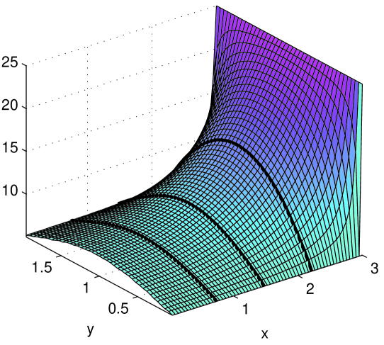
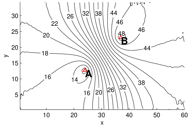
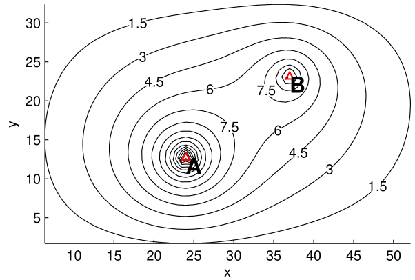
Simulation results. Fig. 6 shows the results of a simulation. The domain consists of a hexagonal array with an approximately rectangular boundary, with cells along the bottom edge and along the left. The fixed disks have radii , the rotating disks , so that each particle hits the rotating disk on average about 10 times before exiting. We place two point sources in the system at the indicated locations. Shown are the disk energy profile and the mean particle count . The discrepancy between predicted and simulation profiles are for and for away from boundaries.
These results are as expected: the disk energy and particle count profiles clearly reflect parameters of the point sources. One also sees clearly that the number of particles tends to zero as one approaches the boundary of the domain, as it should for open boundaries. The sparsity of particles explains the relative noisiness near the boundaries of Fig. 6(a) (as discussed in relation to the left edge in Example 2).
 |
 |
| (a) Mean disk energy | (b) Mean particle count |
Concluding remarks for Section 2
We have extended the recipe for profile prediction proposed in [16] to a variety of situations and tested it in many concrete examples. In each of the three examples presented (and the many others not shown), we have found that (i) the predicted profiles are very simple to compute, and (ii) the discrepancies between predicted and simulated values are no more than a few percentage points. Given that our parameter choices take the systems tested very far out of equilibrium and the system sizes considered are only moderate, we find the agreement between predicted and simulated results strong. We conclude that the scheme proposed is effective for the class of models studied.
3 Memory, finite-size effects, and geometry
The success of the prediction scheme proposed in [16] and extended in Sect. 2 of the present paper prompts the following question: Why is it that memory and finite-size effects have so little impact on macroscopic profiles in the models considered? The purpose of this section is to investigate, in the simpler setting of 1D chains, which dynamical mechanisms and/or aspects of cell geometry are responsible for this outcome, and what happens if the geometry is varied.
We focus on the following two issues:
-
1.
Directional bias due to memory of particle history, i.e., depending on its past history and the state of the cell, a particle may have a preferred direction for exiting; and
-
2.
Incomplete equilibration within cells, which may (or may not) happen when particles collide too few times with the rotating disk before exiting.
3.1 Directional bias due to particle history
The first part of this subsection has some overlap with [15], which contains a phenomenological study of the same bias questions. Our findings are consistent with those in that earlier study, though we take a slightly different approach, and the bias-correction equations we derive (which are simpler than those in [15]) will be tested in models with significant bias.
The 1D-chain used here is exactly one row of the 2D-rectangular configuration used in the previous section, with the top and bottom gaps of each cell sealed, i.e., particles reflect off these two straight segments elastically. In Parts (A) and (B) below, we consider systems with fixed disk radius (leading to gap size ) and rotating disk radius , the same parameters as those used in Examples 1 and 2 of the previous section. These parameters will be varied, with consequences, in Part (C).
The analysis below applies only to situations when there is a sufficient number of particles in the cell. We assume a mean occupation number of at least about 5.
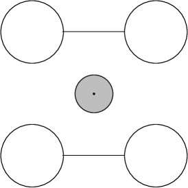
(A) Single cell
We begin by measuring the amount of bias in a single cell using numerical simulations. Consider a array of fixed disks defining a single cell as shown. Heat baths with the following parameters are attached to the left and right openings:
![[Uncaptioned image]](https://cdn.awesomepapers.org/papers/69d1735f-681f-4bea-9721-f2f30dd04935/x15.png) |
||
Let and denote the rates at which particles exit the cell to the left and to the right respectively. Similarly, we denote mean energy outflux rates by , and define the mean “temperatures” of outgoing particles by . We express the observed bias by
Note that zero directional bias would imply .
We then express and in terms of and , stipulating that , and also , be symmetric about . Expanding to leading order, we obtain
| (2) |
where the coefficients are computed (using ) to be333The error estimates given here are standard error (corresponding to 95% confidence intervals). This degree of uncertainty has almost no perceptible effect on the bias correction results in Sect. 3.2(B).
Relevant dynamical mechanisms. In general, we think of the rotating disk, whose energy fluctuates wildly, as a randomizing force, causing particles to lose memory of their previous spatial locations and directions. Without a doubt, this mechanism is responsible for diminishing bias in exit direction.444Concave cell walls also help in the scattering of particles, but they appear not to be as important as the randomizing effects of the rotating disk. There is a situation, however, when this mechanism fails: Suppose a particle enters from the right and hits the rotating disk at roughly a right angle. If the rotating disk at that moment happens to have energy considerably lower than that of the particle, then after the energy exchange (see Sect. 1.1), the normal component of the velocity of the particle continues to dominate its tangential component, and the particle is reflected back essentially the way it came.555A similar observation is made in [15].
Define a reflected particle to be one which, in the course of its journey through the cell, hits only the rotating disk and the two fixed disks on the side of the opening through which it enters, i.e. it is “reflected back”. (Such particles need not exit the first time around; they can turn around and have multiple interactions with the rotating disk.) For and , we find that among particles entering from the left (respectively, the right), a fraction is reflected. Since higher energy particles are more likely to reflect, one naturally expects the mean temperature of reflected particles to be higher than that of other particles. At , we find this difference to be .
Assuming that particles that are not reflected are thoroughly randomized, one would expect, in terms of orders of magnitude, that and . The estimate for is based on the fact that on the side with higher injection rate, a larger fraction of particles is reflected, and this fraction has higher temperature. Computed values of and are consistent with these very naïve estimates. As for , we can only say that it should be because higher temperature leads to more reflected particles.
The findings above support our contention that reflected particles are an important source of bias, but the true story is much more complicated. For example, when a particle interacts with the rotating disk, even as some memory is lost, its post-collision trajectory is not entirely random. It also retains some memory of its previous energy since the normal component of its velocity upon impact is kept. A complete analysis is beyond the scope of this article.
Linear response for general . If bias arises mainly from individual particle trajectories — and that appears to be the case when there is a sufficient number of particles in the cell — and should scale linearly with the total injection rate . This allows us to extend the linear response relation (2) to boundary conditions
for general . The general linear response relations are
| (3) |
where the phenomenological coefficients , , etc., are as in Eq. (2). We have numerically verified that these scaling relations are accurate to within 2% for and .666As pointed out in [15], in principle these coefficients may depend on particle density (this follows from dimensional analysis). We have not found evidence for any significant variation within the range of parameters used here.
(B) Chains
A natural next step is to try to use the linear response relation (3) to account for the effects of bias on macroscopic profiles. A priori, knowledge of bias effects in a single cell need not tell us about how a cell would behave when placed within a chain: single cells are driven by I.I.D. bath injections whereas cells within a chain receive correlated inputs, and long-range correlations are known to be substantial in nonequilibrium steady states.
Prediction scheme with built-in bias correction. We derive phenomenological equations for macroscopic profiles assuming that bias at a given site is determined solely by the temperature, particle flux, and their gradients at , in the same way as in a single cell. Let and be the mean rates of energy and particle flux out of cell , i.e., is the mean total energy that passes from cell to cell per unit time, and so on, and let .
First, we have the balance equations
| (4) |
These are augmented by bias corrections of the same form as Eq. (3):
| (5) |
where we define
and
Our proposal is to first compute the coefficients , , , from single cell simulations, and then to solve Eqs. (4) and (5) numerically to obtain bias-corrected predictions. If , these equations are precisely the prediction scheme outlined in Sect. 1.2.
We have carried out simulations to validate this bias correction scheme. For chains with the cell geometry in Part (A), the effect of bias is generally small but measurable. Even with these more delicate measurements, our scheme gives quite accurate predictions of and . These findings will be corroborated by those in simulation studies for which bias is more significant, which we now discuss.
(C) “Good” geometry, “bad” geometry
Up until now, we have considered a fixed cell geometry (namely that in Fig. 7(a)), which by all counts gives rise to very little bias. One would expect bias to increase for geometries which have a larger fraction of reflected orbits. For example, one may guess that if one increases the gap size , it will be easier for reflected particles to exit, and the bias coefficients will go up. We have found this to be true, provided is somewhat smaller than .
A more straightforward way to increase the fraction of reflected particles, however, is to fix gap size and increase , for larger rotating disks are more effective in blocking incoming orbits. Table 1 shows the values of and for various values of with gap size fixed at , equivalently with . The trends are self-evident.
| r | 0.055 | 0.1 | 0.2 | 0.3 | 0.4 |
|---|---|---|---|---|---|
| 0.060 | 0.13 | 0.23 | 0.33 | ||
| 0.004 | 0.014 | 0.023 | 0.028 |
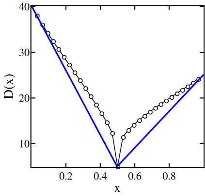
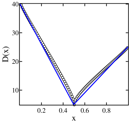
Example 4: A chain with “bad” geometry. We consider here cells with and ; a picture of such a cell is shown in Fig. 7(b). This is a candidate for a “bad” geometry: it is almost as easy for a particle to bounce back and forth between two adjacent cells as it is to pass from a side chamber to the top or bottom chamber of the same cell. Simulations were performed for a chain with , , , , and ; the results are displayed in Fig. 8.
 |
 |
 |
||
| (a) | (b) | (c) |
Predicted profiles using the scheme without bias correction are shown in dashed lines, while bias-corrected profiles are shown as solid lines. As can be seen from the plots, deviations of simulation data (circles) from uncorrected profile predictions are nontrivial, unlike the situations in Examples 1–3, where cell geometries are considerably more favorable. On the other hand, the fit with profiles from our bias-corrected prediction scheme is excellent. These profiles are computed from Eqs. (4) and (5) using coefficients , , , and from single cell simulations with .
 |
 |
|
| (a) Mean disk energy | (b) Mean particle count |
3.2 Incomplete equilibration
When every particle spends a very long time in a cell before moving on, one may expect the particles and the rotating disk in the cell to come close to equilibrating. Thus one may think that small gaps (or passageways) between cells speed up the convergence to local equilibrium. In [16] and [15], these gaps were taken to be very small: on average, a particle hits the rotating disk more than times on each visit to a cell. In Examples 1–3 in the present paper, these conditions are relaxed to 3-5 hits per visit. But are small gaps a necessary condition? Put differently, suppose the gaps are large (as in Fig. 7(c)), so that each particle moves through every cell quickly, hitting the rotating disk only once or twice (or even less) on each pass. Would such incomplete equilibration necessarily lead to anomalous behavior?
We now attempt to address this question. The short answer is: A particle’s failure to completely equilibrate with its cell environment on each pass is, in and of itself, not an obstruction to normal behavior. However, large gaps can amplify finite-size effects.
For lack of a better term, let us call a cell boundary “porous” if a particle passing through the cell is not likely to collide with the rotating disk too many times before exiting. For the type of models discussed earlier, porosity is equivalent to larger gap size. We propose below a connection between porosity and finite-size effects, and provide numerical confirmation of our thinking.
Dynamics of equilibration and finite-size effects: a heuristic discussion
From the point of view of a particle, equilibration takes place as follows: It moves about the chain in what is essentially a random walk, exchanging energy with the rotating disks with which it collides, hence indirectly with other particles which collide with the same disks. It is an ongoing process, a very messy one involving large fluctuations. To say that a particle has “equilibrated” basically means that it has acquired “the right statistics.” From this picture, it is clear that full equilibration in one cell before proceeding to the next is not at all necessary.
However, a particle has to remain in the system long enough to fully sample the totality of its surroundings. For a concrete example, suppose we place a thermostat in the middle of a chain. As noted in Example 2, particles retain their normal components in collisions, one might naively expect that a particle has to interact with the thermostat many times for equilibration to occur. (Actually, it can also acquire this information indirectly.) If the chain is too short and most of the particles exit too quickly, then the thermostat may not be fully effective due to insufficient sampling. In the case of boundary injections, if the domain is not large enough for particles to collide a sufficient number of times before exiting the system, then the different sets of statistics carried by injected particles (e.g., bath temperature) may not have enough opportunity to get absorbed and propagated through the chain.
The phenomena described above can be thought of as incomplete equilibration with thermostats or baths. They will lead to finite-size effects. This kind of equilibration does not require that the particle make many collisions in each cell that it visits, though more collisions are conducive to better statistics.
Here is how porosity enters. To exaggerate the problem, consider a situation where cell boundaries are sufficiently porous that on average particles travel ballistically for some (microscopic) distance without exchanging energy with any disks. In such a system, particles will need more “room” to make the same number of collisions. The more porous the cell boundaries, the greater the mean free path. The discussion above continues to apply, but a longer chain or larger domain is required to ensure complete equilibration with thermostats or baths.
Alternatively, consider a chain of length in which the mean free path of particles is . If we view particles in this chain as moving on the interval , the paths traced out will resemble those of a diffusion whose associated lengthscale increases with (for fixed ) and decreases with (for fixed ). This suggests the following: (a) Incomplete equilibration in an -chain can have a smoothing effect on the profiles of relevant observables on , as though they are convolved with some kernel. In particular, profiles that are strongly curved may lose some of their curvature. (b) Whatever the porosity, this smoothing vanishes as .
The discussion above is entirely heuristic, but we believe it captures the flavor of part of what is going on. To summarize, our reasoning implies the following: (1) Other things being equal, the more porous the cell geometry, the larger the deviation from expected behavior for a fixed system size. (2) In the infinite-volume limit, these effects will vanish, i.e., these are genuinely finite-size effects.
A number of numerical studies were carried out to support (or refute) the thinking above. Chains driven by (unequal) boundary injections behave exactly as described: finite-size effects in the form of decreased curvature are clearly visible but for the most part not too pronounced for chains of moderate length. The thermostat example discussed above provides a more dramatic illustration of complete versus incomplete equilibration.
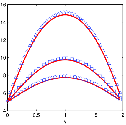
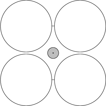
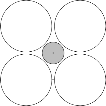
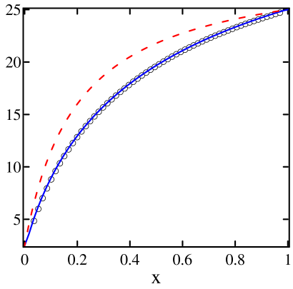
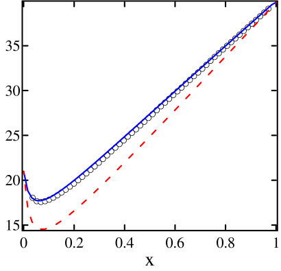
Example 5: Cells without borders. The basic setup is illustrated in Fig. 9(a): it consists of a 1D chain connected to two heat baths at the two ends and with a single thermostated cell in (exactly) the middle. The boundary conditions are , , and , and the thermostat is set to temperature . Neglecting the possible effects of bias, the predictions in Sect. 2 give, in the continuum limit, a piecewise linear profile for the disk energy : it linearly interpolates the 3 values , , and ; particle count is computed as before, i.e. assuming the system is partitioned into cells (with invisible separations), with each cell containing exactly one disk. System size will be varied in this study. We consider the following three cell geometries:
-
•
Geometry A (small gaps): , resulting in gap size , and ; see Fig. 7(a). These are the parameters used in Examples 1–3. The average number of interactions with the rotating disk is per visit.
-
•
Geometry B (large gaps): , resulting in gap size , and , as shown in Fig. 7(c). This configuration has infinite horizon. Number of hits per pass is .
-
•
Geometry C (no walls between cells): and . A chain with this geometry is shown in Fig. 9(a). This is as “porous” a geometry as there can be.
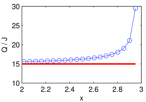
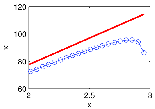
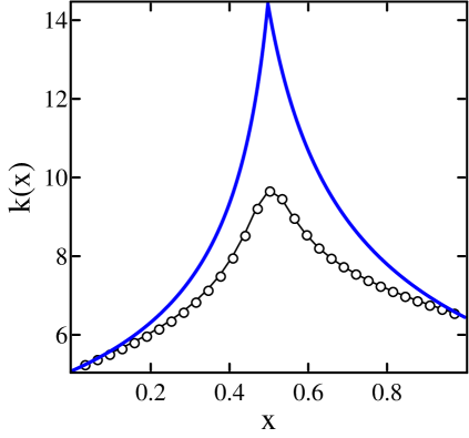
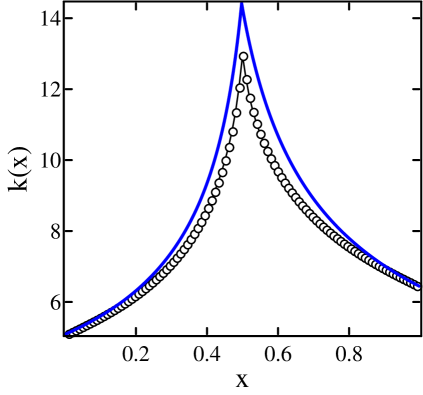
For each of these geometries, we computed and for 31, 61, 121, 201 and 401 (for Geometry C, note that the derivations in Sect. 1.2 are not affected by the fact that there are no cell walls). In each case, deviation from the predicted profile decreases monotonically as the length of the chain increases. Two sets of results for Geometry C are shown in Fig. 9(b). As one can see, finite-size effects are very nontrivial at , and are still clearly visible at . From the plotted values of (set to at on account of the thermostat), one sees that the effectiveness of the thermostat is seriously compromised at : being higher than predicted is consistent with being lower than predicted. The plot of shows unambiguously the effects of smoothing, confirming the incomplete-equilibration-with-thermostat picture proposed. By contrast, the plots for Geometry A (not shown) show no visible finite-size effects beyond ; at , the deviations are already smaller than those for Geometry C at . Simulation results for Geometry B are between those of A and C; they contain no surprises.
(a) Cells without borders
|
 |
|||||||
| (b) Profiles | (c) Disk energy distribution, |
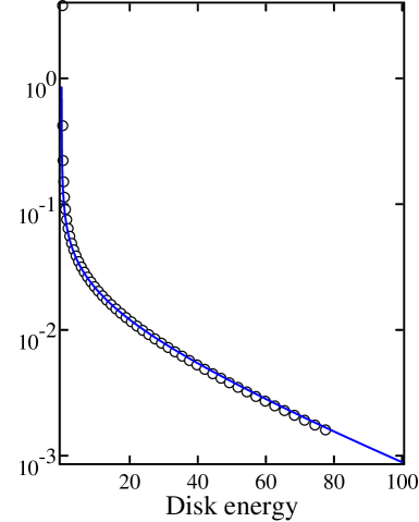
An intriguing question is the distribution of disk energy for this type of chains, for they are the antithesis of chains with tiny gaps (introduced in [16] with the idea that equilibration within cells may lead to more rapid convergence to local equilibrium). A specific question is whether as single site marginals of steady states will tend to measures of the form defined in Sect. 1.1. Numerical evidence suggests that they will: We found that disk energy distributions are of Gibbs form for even fairly short chains, independently of the completeness of equilibration with baths or thermostats. Fig. 9(c) shows the distributions of disk energy at for Geometry C with . The plot is in log-linear scale; data collected from simulations are plotted against disk energy distribution for with and equal to the empirical temperature at the site in question. Notice the remarkable agreement, demonstrating how close these marginals are to some long before approaches its continuum value.
3.3 Implications for general model designs
Building on previous ideas, our results in Sects. 2, 3.1, and 3.2 point to a very rich class of out-of-equilibrium Hamiltonian models for which we have a simple and effective scheme for predicting approximate energy and particle density profiles. We recapitulate here some of the ideas, and discuss further implications.
Retaining the particle-disk interaction introduced in [35] and [27], we have shown that the ideas first put forward in [16] are applicable to a very flexible collection of models:
First, the results are not limited to 1D; simulations have been carried out in 1D and 2D, and we have seen no reason why the type of prediction scheme studied in this paper cannot be applied in three and higher dimensions, provided the models have suitable interactions between moving particles and pinned-down objects. The type of lattices over which to place the rotating disks appears not to be an issue either; we have illustrated it for rectangular and hexagonal lattices. We have tested a number of different ways to maintain the system out of equilibrium: be it boundary driven (we have tested a variety of boundary conditions), or driven from the interior, using point sources or rows of thermostats – in all cases our prediction scheme has produced easy-to-compute profiles that show strong agreement with simulations.
To understand why memory and finite-size effects are so mild in the models tested in [16] and in Sect. 2, we have proposed an explanation in terms of geometric designs: In these models, the cells have mostly concave (scattering) walls, are connected by narrow passageways, and have rotating disks at good distances away from the walls. We have shown in Sect. 3.1, as have the authors of [15] earlier, that such designs give rise to very low degrees of directional bias. We have also explained in Sect. 3.2 that the small passageways, which facilitate equilibration within cells, also ensure the efficient absorption of bath and thermostat information, reducing finite-size effects. This explains to some degree the rather surprising fact that in [16], for example, the prediction scheme gives remarkably good results in chains with a mere 30 cells.
Going beyond the models discussed in the last paragraph, we have found bias to be small even as we relax considerably the parameters there, i.e., Assumption 1 in Sect. 1.1 applies to a quite large collection of models. However, there are equally natural geometries that give rise a non-negligible amount of bias. For these geometries, we have derived a correction scheme which is relatively straightforward to implement, and shown it to give accurate results (see Sect. 3.1). In a different direction, we have produced numerical evidence in support of our ideas on porosity of cell boundaries and finite-size effects (Sect. 3.2). If these heuristic ideas could be further developed and validated, the implications would be that the results in [16] and Sect. 2 of this paper will remain valid for systems with large gap sizes (perhaps no walls at all) – provided we go to larger system sizes.
We finish with two examples: Example 6(A), along with Example 5, represents one of the greatest departures from the models studied in [16] for which our prediction scheme remains effective; Example 6(B), a close cousin of Example 6(A), makes a connection to the models studied in [27].
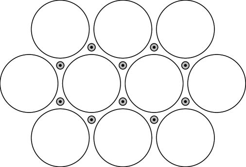
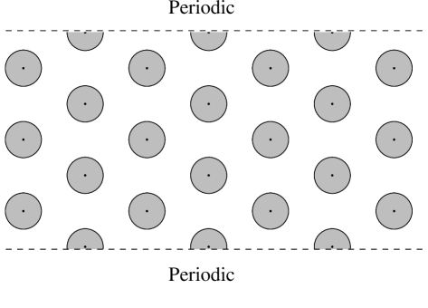
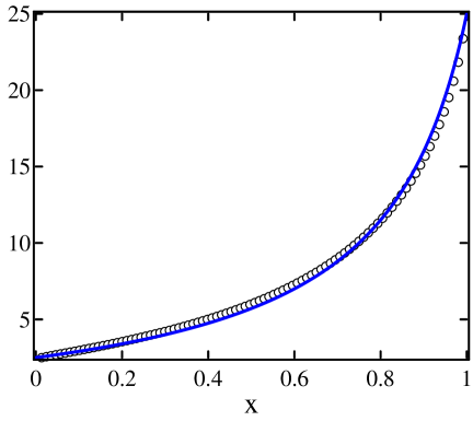
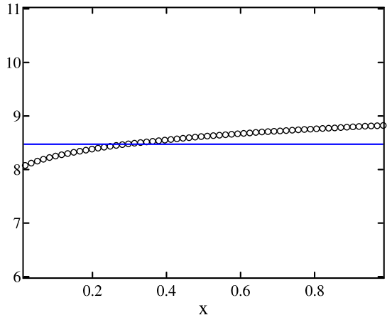
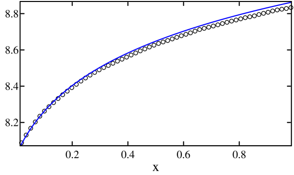
Example 6. (A) We consider a cylindrical domain (or rectangular domain with periodic boundaries in the vertical direction). Inside this domain, rotating disks are placed on a hexagonal lattice with no cell walls or partitions of any kind separating the disks. The disks have radii , and the centers of adjacent disks are 1 unit apart. See Fig. 10(a). Heat baths inject particles into the system from the left and the right. To deduce energy and particle count profiles, we subdivide the domain into hexagonal cells each enclosing exactly one rotating disk in its center, and proceed as before. Fig. 10(b) shows the computed disk energy profile (open circles) and the predicted profile (without bias correction) for a system consisting of a hexagonal array, with and . A few other sets of parameters besides this one were also tested, with results ranging from good to very good.
(B) The configuration in Fig. 10(a) is reminiscent of the model used in [27], except that the rotating disks in [27] are placed much closer to each other. In (A), we have deliberately kept them apart to avoid bias, which for this geometry can be large: We have carried out a simple experiment similar to that in Sect. 3.1(A) involving 3 rotating disks of radius , separated by 3 narrow channels of width 0.05. When all 3 disks are thermostated at , simulations show that a particle entering the triangular region between the disks through one of the channels is 3-4 times more likely to exit from the same channel than either one of the other two channels. This suggests that a system such as the one in (A) but with disks packed this close will exhibit significant bias. Preliminary testing confirms this thinking. For example, when , the profile for , which in the absence of bias would be constant along the length of the cylinder, was found to be nontrivially curved (concave).
 |
 |
|
| (a) Hexagonal grid without cell borders | (b) Mean disc energies vs. |
Remark. Finally, we observe that as far as methods and overall ideas are concerned, no aspect of our studies is tied to the particle-disk interaction used. Thus it is reasonable to conjecture that they may extend to other suitable short-range interactions.
4 Systems with constant particle number
Up to this point in the paper, we have studied nonequilibrium steady states in systems where both particles and energy can flow across the boundary, with bath injection rates and playing the role of chemical potentials. In this section, we consider systems in which the total particle count is maintained at a constant number, and only energy is allowed to flow into and out of the system. The difference between these particle-conserving chains and the chains we studied earlier is akin to the difference between canonical and grand canonical ensembles in equilibrium statistical mechanics.
To keep the number of particles fixed in models of the type studied in [16] and in this paper, one way is to replace particles upon their reaching the boundary of the domain with new particles whose energies reflect those of the baths. That is to say, each particle that exits is replaced instantaneously by a new one, and there is no other infusion of particles. Another possibility is to isolate the system entirely from its surroundings, and to place in different parts of the domain thermostats set to unequal temperatures. Below, we report on findings using particle-conserving baths; we have found that simulations using thermostats yield similar results.
Example 7: 1D-chain with particles replaced on exit
We consider a 1D -chain as before, with cells and being in contact with heat baths. Particles are replaced immediately upon exit. To be definite, we assume that when a particle exits the system at location , where is either the left opening of cell or the right opening of cell , independently of its exit velocity it is replaced by a new particle which appears in the same position and has a new velocity sampled from the bath distribution in Eq. (1). Equivalently, one can think of the gaps leading outside the chain as being sealed off by two “thermostated walls,” and when a particle hits one of these walls, it is reflected but with a new velocity. With these particle-conserving dynamics, the total number of particles remains constant in time. Taking a continuum limit means letting while keeping the density constant.
Profile prediction. We submit that the various profiles can still be predicted following the basic recipe in Sect. 1.2: one first solves for the mean particle jump rate and the mean energy outflux ; the other profiles are then expressed in terms of and as before.
What is different here is that because particles are replaced upon exit, the boundary conditions for are and . These (discrete) homogeneous Neumann boundary conditions lead, assuming zero bias, to , i.e., the profile is constant in space. The profile has the same boundary conditions as before and is linear. This leads to a linear temperature profile. The solutions to the and equations are unique only up to multiplicative constants: they are scaled to match the total particle number in the chain.
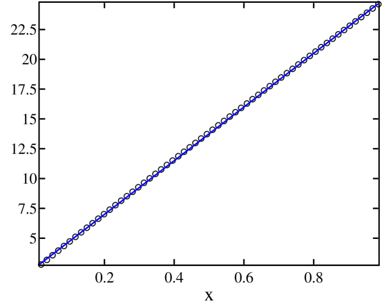
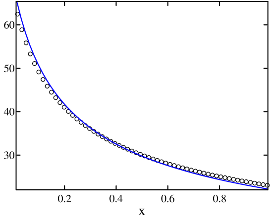
Simulation results. Fig. 11(a) shows simulation results for a chain with and , and boundary conditions and . Shown are simulation data (dots) and predicted profiles – without any built-in bias correction. As can be seen, the agreement is very good except for the profile.
|
|
|
| (a) Simulation and predicted profiles without bias correction | ||
(b) Bias-corrected profile
The discrepancy in the profile is, at first, a little puzzling: it is somewhat larger than in similar non-particle-conserving chains, and is not improved by doubling the total number of particles to . At the same time, estimates along the lines discussed in Sect. 3.1 show that the amount of bias here () is relatively small. A possible explanation is that in the present setting, bias can and does lead to a net gradient in across the length of the chain, whereas in non-particle-conserving systems the values of at the two ends are fixed by the baths.
Fig. 11(b) shows bias-corrected predictions for using the same numerical values of the bias coefficients , , etc., as in Sect. 3. Agreement with simulation data is good, and lends further support to the idea that bias is a “local” phenomenon, governed mainly by the mean values of thermodynamic quantities and their gradients.
Conclusions
The main findings of this paper are:
-
1.
For a large class of Hamiltonian systems, macroscopic profiles such as those for energy and particle count can be quite accurately predicted in a simple way. The scheme introduced in [16] and applied to 1D chains is extended here to more general settings, including 2D systems on rectangular and hexagonal lattices driven by Dirichlet and other boundary conditions, even point sources. Strong agreement with simulation data is also obtained for systems regulated by thermostats, and for systems in which particle numbers are held constant.
-
2.
Memory effects resulting in directional bias of particle trajectories can vary from negligible to significant depending on cell geometry. Where such bias is weak, as is the case for a range of examples, the prediction scheme above (which assumes zero bias) gives accurate results. For “bad” geometries, a scheme with built-in bias correction is shown to be effective.
-
3.
Porous cell boundaries (or large gaps) cause finite-size effects to become more pronounced due to incomplete equilibration with baths or thermostats but do not otherwise appear to impact macroscopic profiles or LTE.
A more detailed discussion of (ii) and (iii) is given in Sect. 3.3.
Acknowledgement.
We are grateful to the referee for many detailed and helpful comments.
References
- [1] P. Balint, K. K. Lin, L.-S. Young, “Ergodicity and energy distributions for some boundary driven integrable Hamiltonian chains,” to appear in Commun. Math. Phys. (2009)
- [2] L. Bertini; A. De Sole; D. Gabrielli; G. Jona-Lasinio; C. Landim, “Stochastic interacting particle systems out of equilibrium,” J. Stat. Mech.: Theory Exp. (2007) P07014
- [3] L. Bertini, A. De Sole, D. Gabrielli, G. Jona-Lasinio, C. Landim, “Macroscopic fluctuation theory for stationary non-equilibrium states,” J. Statist. Phys. 107 (2002) pp. 635–675
- [4] L. Bertini, D. Gabrielli, J. L. Lebowitz, “Large deviations for a stochastic model of heat flow,” J. Stat. Phys. 121 (2005) pp. 843–885
- [5] F. Bonetto, J. L. Lebowitz, J. Lukkarinen, and S. Olla, “Heat conduction and entropy production in anharmonic crystals with self-consistent stochastic reservoirs,” preprint (2009)
- [6] F. Bonetto, J. Lebowitz, and L. Rey-Bellet, “Fourier law: a challenge to theorists,” in Mathematical Physics 2000, edited by A. Fokas, A. Grigoryan, T. Kibble, and B. Zegarlinski, Imp. Coll. Press, London (2000)
- [7] J. Bricmont and A. Kupiainen, “Towards a derivation of Fourier’s law for coupled anharmonic oscillators,” Commun. Math. Phys. 274 (2007) 555–626
- [8] N. I. Chernov, G. L. Eyink, J. L. Lebowitz, Ya. G. Sinai, “Steady-state electrical conduction in the periodic Lorentz gas,” Commun. Math. Phys. 154 (1993) pp. 569–601
- [9] P. Collet and J.-P. Eckmann, “A model of heat conduction,” Commun. Math. Phys. 287 (2009) pp. 1015–1038
- [10] P. Collet, J.-P. Eckmann, and C. Mejía-Monasterio, “Superdiffusive heat transport in a class of deterministic one-dimensional many-particle Lorentz gases,” preprint (2008)
- [11] B. Derrida, “Non-equilibrium steady states: fluctuations and large deviations of the density and of the current,” J. Stat. Mech. (2007) P07023
- [12] B. Derrida, J. L. Lebowitz, and E. R. Speer, “Large deviation of the density profile in the steady state of the open symmetric simple exclusion process,” J. Statist. Phys. 107 (2002) pp. 599–634
- [13] J.-P. Eckmann and M. Hairer, “Non-equilibrium statistical mechanics of strongly anharmonic chains of oscillators,” Commun. Math. Phys. 212 (2000) pp. 105–164
- [14] J.-P. Eckmann and P. Jacquet, “Controllability for chains of dynamical scatterers,” Nonlinearity 20 (2007) 1601–1617
- [15] J.-P. Eckmann, C. Mejía-Monasterio, E. Zabey, “Memory effects in nonequilibrium transport for deterministic Hamiltonian systems,” J. Stat. Phys. 123 (2006) pp. 1339–1360
- [16] J.-P. Eckmann, L.-S. Young, “Nonequilibrium energy profiles for a class of 1-D models,” Commun. Math. Phys. 262 (2006) pp. 237–267
- [17] D. J. Evans and G. P. Morriss, Statistical Mechanics of Nonequilibrium Liquids, Academic Press (1990)
- [18] G. Gallavotti, “On thermostats: isokinetic or Hamiltonian? Finite or infinite?” Chaos 19 (2009) 013101
- [19] G. Gallavotti and E. G. D. Cohen, “Dynamical ensembles in stationary states,” J. Statist. Phys. 80 (1995) pp. 931–970
- [20] G. Gallavotti and E. Presutti, “Thermodynamic limit for isokinetic thermostats,” preprint (2009) arXiv:0908.3060v1
- [21] P. Gaspard and T. Gilbert, “Heat conduction and Fourier’s law in a class of many particle dispersing billiards,” New J. Phys. 10 (2008) 103004
- [22] S. R. de Groot, P. Mazur, Non-equilibrium Thermodynamics, North-Holland (1962)
- [23] M. Hairer and J. C. Mattingly, “Slow energy dissipation in systems of anharmonic oscillators,” Commun. Pure Applied Math. 62 (2009) pp. 999–1032
- [24] W. G. Hoover, Computational Statistical Mechanics, Elsevier (1991)
- [25] C. Kipnis, C. Landim, Scaling Limits of Interacting Particle Systems, Berlin: Springer-Verlag (1999)
- [26] C. Kipnis, C. Marchioro, E. Presutti, “Heat flow in an exactly solvable model,” J. Stat. Phys. 27 (1982) pp. 65–74
- [27] H. Larralde, F. Leyvraz, C. Mejía-Monasterio, “Transport properties of a modified Lorentz gas,” J. Stat. Phys. 113 (2003) pp. 197–231
- [28] J. L. Lebowitz and H. Spohn, “A Gallavotti-Cohen-type symmetry in the large deviation functional for stochastic dynamics,” J. Statist. Phys. 95 (1999) pp. 333–365
- [29] S. Lepri, R. Livi, and A. Politi, “Thermal conduction in classical low-dimensional lattices,” Physics Reports 377 (2003)
- [30] S. Lepri, C. Mejía-Monasterio, and A. Politi, “A stochastic model of anomalous heat transport: analytical solution of the nonequilibrium steady state,” J. Phys. A: Math Theor. 42 (2009) 025001
- [31] B. Li, G. Casati, J. Wang, and T. Prosen, “Fourier Law in the alternate-mass hard-core potential chain,” Phys. Rev. Lett. 92 (2004) 254301
- [32] K. K. Lin and L.-S. Young, “Correlations in nonequilibrium steady-states of random-halves models,” J. Stat. Phys. 128 (2007) pp. 607–639
- [33] C. Mejía-Monasterio and L. Rondoni, “On the fluctuation relation for Nosé-Hoover boundary thermostated systems,” J. Stat. Phys. 133 (2008)
- [34] S. Olla, S. R. S. Varadhan, and H. T. Yau, “Hydrodynamical limit for a Hamiltonian system with weak noise,” Commun. Math. Phys. 155 (1993) 523-560
- [35] K. Rateitschak, R. Klages, and G. Nicolis, “Thermostating by deterministic scattering: the periodic Lorentz gas,” J. Stat. Phys. 99 (2000) 1339–1364
- [36] K. Ravishankar and L.-S. Young, “Local thermodynamic equilibrium for some stochastic models of Hamiltonian origin,” J Stat. Phys. 128 (2007) 641–665
- [37] L. Rey-Bellet, “Nonequilibrium statistical mechanics of open classical systems,” in XIVth International Conference on Mathematical Physics, World Scientific (2006)
- [38] L. Rey-Bellet and L. E. Thomas, “Asymptotic behavior of thermal non-equilibrium steady states for a driven chain of anharmonic oscillators,” Commun. Math. Phys. 215 (2000) 1–24
- [39] D. Ruelle, “Positivity of entropy production in the presence of a random thermostat,” J. Statist. Phys. 86 (1997) pp. 935–951
- [40] D. Ruelle, “Nonequilibrium statistical mechanics and entropy production in a classical infinite system of rotators,” Commun. Math. Phys. 270 (2007) pp. 233–265
- [41] D. Ruelle, “What physical quantities make sense in nonequilibrium statistical mechanics?” in Boltzmann’s Legacy, edited by G. Gallavotti, W. L. Reiter, J. Yngvason, European Mathematial Society, Zürich (2008), pp. 89–97
- [42] D. Ruelle, “A review of linear response theory for general differentiable dynamical systems,” Nonlinearity 22 (2009) pp. 855–870
- [43] H. Spohn, “Long range correlations for stochastic lattice gases in a nonequilibrium steady state,” J. Phys. A 16 (1983) pp. 4275–4291
- [44] H. Spohn, Large Scale Dynamics of Interacting Particles, Texts and Monographs in Physics, Springer-Verlag (1991)