Nonlinear dynamics of topological Dirac fermions in 2D spin-orbit coupled materials

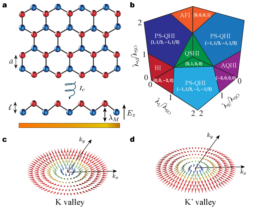
Graphene is the typical go-to material to investigate the optoelectronic response of two-dimensional (2D) systems Neto2009 ; Peres2010 because of its extraordinary electron mobility Graphenereview , tunable linear electronic conductivity Tunable2011 , and potential for strong-light matter interactions at sub-wavelength scales Grapheneplasmons . Although it supports quantum Hall states in the presence of strong magnetic fields QHall1 ; QHall2 ; QHall3 , the intrinsically weak spin-orbit coupling WeakSOC severely limits graphene’s suitability to study topological phase transitions TI1 ; TI2 in low-dimensional materials. The search for alternative topologically non-trivial 2D structures with characteristics similar to graphene recently ended with the synthesis of silicene Silicene , germanene Germanene , stanene Stanene , and plumbene Plumbene . The newer members of the graphene family materials (GFM) have a buckled honeycomb lattice with silicon, germanium, tin, or lead atoms occupying the lattice sites Gomez2016 ; Molle:2017aa ; Mannix:2017aa . Unlike graphene, the strong spin-orbit coupling in these systems results in a gapped bulk energy band-structure and protected one-way edge states characteristic of topological insulators. Strikingly, they can be driven through a variety of phase transitions (Fig. 1a,b) by actively controlling the mass gap via external interactions EzawaJapanese , which could enable unprecedented all-in-one material multi-optoelectronic functionalities with potential applications to spintronics and valleytronics.

Various recent works have investigated ultrafast and nonlinear effects in topologically trivial 2D materials Gnonlinear1 ; Mikhailov2008 ; Kerr ; Gnonlinear2 ; Transition ; Exp2 ; Exp3 ; Exp4 ; Exp5 ; Sipe2014 ; Sipe2015 ; Pedersen2016 ; Mikhailov2016 ; HHG1 ; Lysne2020 ; Linear1 and in topological systems HHG4 ; HHG5 ; HHG6 ; Chacon2020 ; RSeq . Unravelling the interplay between topology and nonlinear effects in spin-orbit coupled monolayer semiconductors of the graphene family is a natural step at the materials science forefront, which could aid in developing next-generation technologies that meet the urgent demands for, among others, higher performance radio-frequency modulators, optically gated transistors, and practical spintronic-based devices. Nevertheless, studies on the optoelectronic properties of these materials have largely focused in their linear responseTunablebandgap1 ; Tunablebandgap2 ; WiltonPRB ; WiltonPRL ; WiltonNonlocal ; Circular3 ; Wiltonnature ; Tabert2014 ; Farias2018 ; Wu2018 ; Wu2020 , which include investigations of signatures of the tunable band gap Tunablebandgap1 ; Circular3 , spatial dispersion Tabert2014 ; WiltonNonlocal , the interplay between the quantum Hall effect Tunablebandgap2 and photo-induced topology WiltonPRB , as well as of topological phase transitions in quantum forces Wiltonnature ; Farias2018 , spin-orbit photonic interactions WiltonPRL , and light beam shifts Wu2018 ; Wu2020 . The crossroads between nonlinear dynamics and topology in the extended graphene family, potentially allowing access to topological phase transition signatures, material symmetries, selection rules, and relaxation mechanisms otherwise screened by spurious effects in the linear response, remains uncharted.

We explore the interplay between topological Dirac fermions in the GFM and optical fields beyond the linear regime. We develop a comprehensive and unified description of their nonlinear dynamical conductivity tensor, including non-trivial topological phases due to an externally applied electrostatic field, a circularly polarized laser, and exchange interaction. Our results show a rich structure of nonlinear optoelectronic responses across the phase diagram, and we demonstrate that the third-order optoelectronic conductivity contribution to the fundamental and third-harmonics encodes fingerprints of topological phase transitions. We show that characterization of the Chern number is possible near bandgap resonances via polarization sensitive detection of the cross-polarized component of the field harmonics. Our work sets the cornerstones for investigating topological phase transitions beyond the linear response in the family of graphene-like elemental 2D materials.

Results

Topological properties of the graphene family - Let us consider the following Dirac-like Hamiltonian describing staggered GFM in the low-energy regime EzawaJapanese ,

$${\hat{H}}_{s}^{\eta}={\bm{\tau}}\cdot{\bf d}^{\eta}_{s}=\hbar v_{F}(\eta k_{x}\tau_{x}+k_{y}\tau_{y})+\Delta_{s}^{\eta}\tau_{z},$$

(1)

where ${\bf d}^{\eta}_{s}=\{\eta\hbar v_{F}k_{x},\hbar v_{F}k_{y},\Delta_{s}^{\eta}\}$ describes a meron structure in momentum space (Fig. 1c,d), $\hat{\textbf{p}}=\hbar(k_{x},k_{y})$ is the particle momentum, $\tau_{i}$ are the Pauli matrices, $\eta,s=\pm 1$ are valley and spin indexes, $v_{F}$ is the Fermi velocity, and the mass term $\Delta_{s}^{\eta}=\eta s\lambda_{SO}-\lambda_{E}-\eta\lambda_{L}+s\lambda_{M}$ corresponds to half energy band gap. Here, $\lambda_{SO}$ represents the intrinsic spin-orbit coupling energy and the last three terms in $\Delta_{s}^{\eta}$ account for interactions with external fields, which allow for tailoring the Dirac mass gap. Indeed, the second term $\lambda_{E}$ corresponds to the potential difference between sub-lattices in the buckled structure in the presence of a static electric field $E_{z}$ applied perpendicularly to the plane of the monolayer Tunablebandgap1 . The third component $\lambda_{L}$ describes the anomalous quantum Hall effect and arises due to the coupling between an off-resonant circularly polarized laser and the GFM Circular2 ; Tunablebandgap2 . The final term $\lambda_{M}$ depicts the staggered antiferromagnetic exchange interaction Antiferromagnetic . For simplicity, we have neglected Rashba couplings due to their small magnitude compared to the other contributions. It is worth mentioning that the Hamiltonian in Eq. (1) applies more generally to other 2D systems, including antiferromagnetic manganese chalcogenophosphates (MnPX₃, X = S, Se) Li and perovskites Liang . The formalism developed here is also valid for these systems.

Within the Dirac picture the electronic properties of the GFM can be fully characterized through a set of four topological invariants EzawaJapanese , namely the Chern ${\cal C}=\sum_{\eta,s}{\cal C}_{s}^{\eta}$, spin Chern ${\cal C}_{s}=\sum_{\eta,s}s\leavevmode\nobreak\ {\cal C}_{s}^{\eta}/2$, valley Chern ${\cal C}_{\eta}=\sum_{\eta,s}\eta\leavevmode\nobreak\ {\cal C}_{s}^{\eta}$, and spin-valley Chern $C_{s\eta}=\sum_{\eta,s}\eta s\leavevmode\nobreak\ {\cal C}_{s}^{\eta}/2$ numbers. Here ${\cal C}_{s}^{\eta}=\eta\leavevmode\nobreak\ \text{sign}[\Delta_{s}^{\eta}]/2$ is the Pontryagin number TI1 ; TI2 , a topological quantity that counts how many times the vector ${\bf d}^{\eta}_{s}/|{\bf d}^{\eta}_{s}|$ wraps a sphere in momentum space (Fig. 1c,d). By varying the external parameters $\lambda_{E},\ \lambda_{L}$, and $\lambda_{M}$ the monolayer can be driven through various phase transitions as depicted in Fig. 1b, where we show the topological phases in the planes $\lambda_{E}=0$, $\lambda_{L}=0$, and $\lambda_{M}=0$. The electronic states quantum spin Hall insulator (QSHI), anomalous quantum Hall insulator (AQHI), band insulator (BI), antiferromagnetic insulator (AFI), and polarized- spin quantum Hall insulator (PS-QHI) have non-zero mass gaps for all four Dirac cones. The system undergoes a topological phase transition when the band gap of at least one Dirac cone changes sign. Hence, the boundaries between insulating states are determined by the condition $\Delta^{\eta}_{s}=0$, which defines the so called single Dirac cone phases (diagonal solid lines in Fig. 1b). At the intersection between boundary lines there are two Dirac gaps closed, and the system is either in a spin, valley, or spin-valley polarized semimetal state. Finally, note that there are four points in the 3D phase diagram, $\{\lambda_{E}/\lambda_{SO},\lambda_{L}/\lambda_{SO},\lambda_{M}/\lambda_{SO}\}=\{-1,-1,1\},\ \{1,1,1\},\ \{1,-1,-1\},\ \{-1,1,-1\}$, where three Dirac cones simultaneously close, corresponding to unique electronic states that remain unexplored to date.

Nonlinear light-matter interactions in the GFM - The nonlinear dynamics of charge carriers in a given Dirac cone interacting with a linearly polarized electromagnetic plane wave impinging normally on the monolayer can be described via the density matrix ${\hat{\rho}}(t)$, which satisfies the equation of motion $i\hbar\ \partial\hat{\rho}(t)/\partial t=\left[{\hat{H}}_{s}^{\eta}+\hat{H}_{i}(t),\hat{\rho}(t)\right]-\Gamma({\hat{\rho}(t)}-{\hat{\rho}}^{(0)}).$ Here, $\hat{H}_{i}(t)=e{\hat{\bm{p}}}\cdot{{\bm{A}}}(t)/mc$ is the field-monolayer interaction Hamiltonian in the velocity gauge Sipevelocity , where ${\bm{A}}(t)=A(t)\hat{\textbf{x}}$ is the electromagnetic vector potential. We assume that at large times the system relaxes to the equilibrium density matrix $\hat{\rho}^{(0)}=\sum_{l,{\bm{k}}}f_{l{\bm{k}}}|l{\bm{k}}\rangle\langle l{\bm{k}}|$ with a phenomenological decay rate $\Gamma$, where $f_{l{\bm{k}}}$ is the Fermi-Dirac distribution for fermions in the valence or conduction bands ($l=\pm 1$) with momentum $\hbar\textbf{k}$, and $|l{\bm{k}}\rangle$ are the corresponding eigenstates of the unperturbed Hamiltonian $H^{\eta}_{s}$ (see Methods). In general, the equation of motion cannot be solved analytically due to the time dependence of the interaction Hamiltonian, and numerical methods are often employed. Here, instead, we use perturbation theory by expanding the density matrix ${\hat{\rho}}(t)=\sum_{n}{\hat{\rho}}^{(n)}(t)$ in powers of the vector potential amplitude and iteratively solve for $\rho^{(n)}(t)\propto A(t)^{n}$. We use the standard expression for total current ${\bm{j}}(t)=-e{\text{T}r}[{\hat{\rho}}(t)({\hat{\bm{v}}}+\frac{e}{mc}{\hat{\bm{A}}}(t))]$, which contains contributions arising from all orders in the perturbative expansionPedersen2017 ; Aversa1995 . Here, $\hat{v}=\hbar^{-1}\nabla_{{\bf k}}\hat{H}_{s}^{\eta}$ is the velocity operator. The $n$-th order ac electric current is given by

$${\bm{j}}^{(n)}(t)=-e\textrm{Tr}[{\hat{\rho}}^{(n)}(t){\hat{\bm{v}}}]-\frac{e^{2}}{mc}\textrm{Tr}[{\hat{\rho}}^{(n-1)}(t){\bm{A}}(t)].$$

(2)

Although the last term in the previous equation does not vanish in general, one can demonstrate that it is exactly canceled by another contribution arising from the first term and, therefore, its contributions do not appear in the final expressions for the conductivities. The cross-canceling of contributions involving the first and second terms in Eq. (2) is actually critical to reobtain the well know expression for the conductivity in the linear regime, given by Kubo’s formalism (Methods). The $n$-th order optical conductivity is a tensor of rank $n+1$, accounts for both intra and interband transition contributions as well as topological effects emerging from the Berry connection EzawaJapanese , and can be directly computed after Fourier transforming the above equation and expressing the current as a product between the electric field and conductivity.

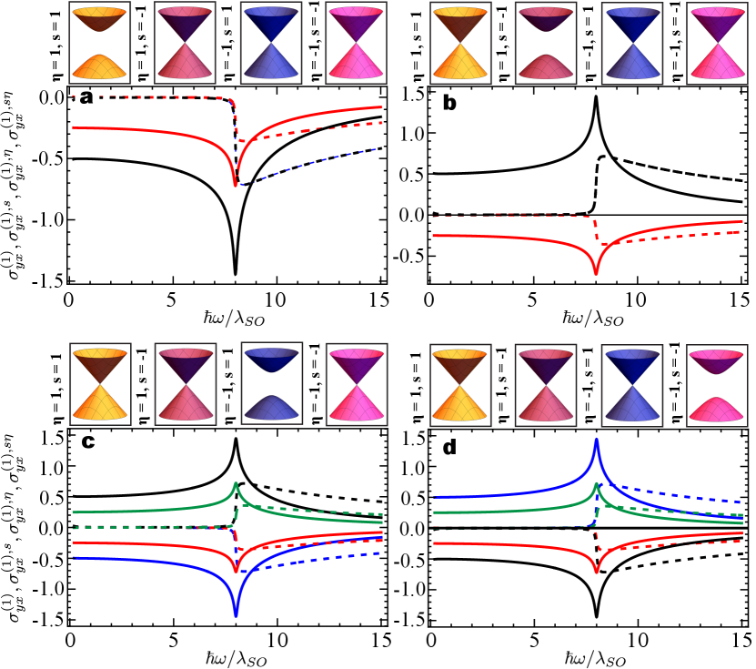
The longitudinal $\sigma_{xx}^{(1)\eta,s}(\omega)$ and transverse $\sigma_{yx}^{(1)\eta,s}(\omega)$ linear optical conductivities per Dirac cone obtained from Eq. (2) are in full accordance with previous studies, and have been investigated in details in the $\lambda_{M}=0$ plane in Refs. 33, 41, 49, 47. For completeness, we explore in Fig. 2 the charge, spin, valley, and spin-valley transverse linear conductivities (summed over valley and spin indexes as shown in the Methods) in the four phases with only one Dirac cone open, since these have been previously overlooked in the literature. By measuring the dynamic linear conductivities at these unique points in phase space one can investigate topological properties emerging from each Dirac cone individually. Indeed, the nonzero Dirac gap in each of the cases considered leads to Chern numbers ${\cal C}$, ${\cal C}_{\eta}$ $=\pm 1/2$, and ${\cal C}_{s}$, ${\cal C}_{s\eta}$ $=\pm 1/4$, which clearly manifest in the zero frequency limit of the transverse conductivities for neutral monolayers, as shown in Fig. 2. Note that in panels 2a,b the charge (spin) and the valley (spin-valley) currents are identical, which implies that the nonzero Dirac gap belongs to the $K$ valley, while in panels 2c,d the charge (spin) and valley (spin-valley) conductivities are the negative of each other, hence the nonzero Dirac gap belongs to $K^{\prime}$ valley. Finally, the sign of the spin or spin-valley linear conductivities in the quasi-static regime allows to identify the spin of the charge carriers.

The second order response of the system described by the Hamiltonian in Eq. (1) vanishes due to the centrosymmetry of the GFM. The first nonlinear contribution comes from the third-order response and can be described by a rank four conductivity tensor $\tilde{\sigma}_{\alpha\beta\gamma\delta}^{(3)\eta,s}(\omega_{1},\omega_{2},\omega_{3})$, which is invariant under simultaneous permutations of the indexes $\beta,\gamma,\delta$ and frequencies $\omega_{1},\omega_{2},\omega_{3}$, where $\alpha,\beta,\gamma,\delta=x,y$ (see Methods). For simplicity we will concentrate in cases where $\beta=\gamma=\delta=x$ and we will assume that the incident electromagnetic radiation is monochromatic, i.e., ${\bm{A}}(t)=A_{0}\cos(\omega t)\leavevmode\nobreak\ \hat{\textbf{x}}$, allowing us to separated the third-order conductivity into terms oscillating with frequencies $\omega$ and $3\omega$. The first term adds to the linear conductivity response and gives a correction to the fundamental harmonic that is quadratic in the vector potential amplitude (Kerr effect), while the second one describes the nonlinear process of third harmonic generation. Therefore, up to third-order in perturbation theory, the optoelectronic conductivity of the system at the fundamental and third-harmonics due to each Dirac mass gap can be cast as

	$\displaystyle\tilde{\sigma}_{\alpha x}^{\eta,s}(\omega,I_{0})$	$\displaystyle=$	$\displaystyle\sigma_{\alpha x}^{(1)\eta,s}(\omega)+\frac{6\pi}{c}I_{0}\sigma_{\alpha x}^{(3)\eta,s}(\omega),$
	$\displaystyle\tilde{\sigma}_{\alpha x}^{\eta,s}(3\omega,I_{0})$	$\displaystyle=$	$\displaystyle\frac{2\pi}{c}I_{0}\sigma_{\alpha x}^{(3)\eta,s}(3\omega)\,,$		(3)

where $I_{0}=\omega^{2}A_{0}^{2}/8\pi c^{2}$ is the incident field intensity and $\tilde{\sigma}_{\alpha x}^{(3)\eta,s}(\omega)\!\!=\!\!\tilde{\sigma}_{\alpha xxx}^{(3)\eta,s}(\omega,\omega,-\omega)$, $\tilde{\sigma}_{\alpha x}^{(3)\eta,s}(3\omega)\!\!=\!\!\tilde{\sigma}_{\alpha xxx}^{(3)\eta,s}(\omega,\omega,\omega)$ is a shorthand notation. In the next section we discuss topological fingerprints embedded in these nonlinear conductivities.

Topological signatures in the GFM nonlinear response - Let us first look into topological signatures buried in the phase of the optical field by investigating the polarization state (helicity) of light resulting from third-harmonic generation processes. We consider the low temperature regime for a neutral monolayer, i.e., the Fermi level lies in the middle of the band gap, and assume $\hbar\omega=0.2\lambda_{SO}$ and $\hbar\Gamma=0.05\lambda_{SO}$. In Fig. 3a we plot the phase diagram associated with the difference $h_{3\omega}=(I_{L}^{(3)}-I_{R}^{(3)})/I_{0}\propto\text{Im}\left[\sigma_{xx}^{(3)}(3\omega)^{*}\sigma_{yx}^{(3)}(3\omega)\right]$ between intensities $I_{L}^{(3)}$ and $I_{R}^{(3)}$ of light emitted with left and right circular polarization at frequency $3\omega$, respectively, where here the conductivities $\sigma_{xx}^{(3)}(3\omega)$, $\sigma_{yx}^{(3)}(3\omega)$ account for all Dirac cones (Methods).

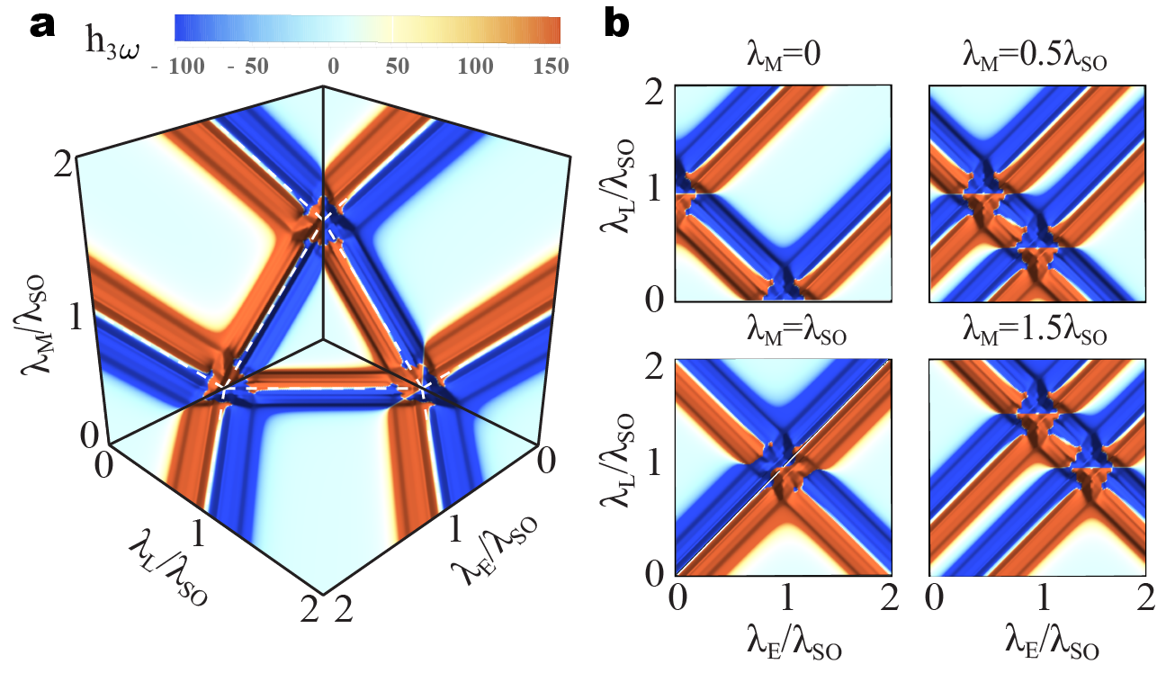
A direct comparison with the phase diagram in Fig. 1 clearly reveals the role of topology in the nonlinear optical response of the GFM. Far from the phase boundaries the contribution from each Dirac gap to $h_{3\omega}$ decreases as $1/|\Delta_{s}^{\eta}|^{4}$, resulting in weak variations of helicity in the middle of the QSHI, BI, AQHI, PS-QHI, and AFI phases.

The effects of nonlinearity are most relevant as one approaches the semi-metallic states (white dashed lines) marking the boundary between different Chern numbers, where $h_{3\omega}$ is dominated by the contribution from the Dirac cone with the smallest gap and the phase transition can be easily identified. These conclusions are not restricted to the planes $\lambda_{E}=0$, $\lambda_{L}=0$, and $\lambda_{M}=0$ as can be seen in Fig. 3b, where we present slices of the phase diagram corresponding to fixed values of $\lambda_{M}$. Note in these panels that as $\lambda_{M}$ increases the phase boundaries come closer to each other and at $\lambda_{M}/\lambda_{SO}=1$ the three phase boundaries cross at a single point, $\{\lambda_{E}/\lambda_{SO},\lambda_{L}/\lambda_{SO},\lambda_{M}/\lambda_{SO}\}=\{1,1,1\}$, corresponding to the closing of three Dirac gaps. Finally, we mention that the variations of $h_{3\omega}$ across a phase transition depend on whether the initial and final phases have trivial charge transport properties (Chern number ${\cal{C}}$ equal to zero). For instance, in the $\lambda_{M}=0$ we observe that $h_{3\omega}$ is a symmetric function around $\lambda_{E}/\lambda_{SO}=1$ when we consider the topological phase transition between the QSHI and BI phases, both with ${\cal{C}}=0$. On the other hand, a remarkably asymmetric behavior takes place around $\lambda_{L}/\lambda_{SO}=1$ (which is energetically equivalent to the previous case) when one considers a topological phase transition involving the QSHI and the AQHI (${\cal{C}}=-2$) phases.

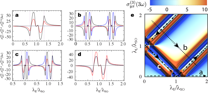
The phase diagram of $h_{3\omega}$ includes contributions from both third-harmonic longitudinal and transverse conductivities. However, only the latter encodes topological features of the GFM and deserves to be independently studied. To this end one could, for instance, use a linear polarizer filter to block the co-polarized scattered field and detect only its cross-polarized component, which is proportional to $\sigma_{yx}^{(3)}$. In Fig. 4 we investigate the charge conductivity $\sigma_{yx}^{(3)}(3\omega)$ along various paths in the phase diagram (parametrized in terms of $\lambda_{E}/\lambda_{SO}$). For completeness we also show the associated spin $\sigma_{yx}^{(3),\textrm{s}}(3\omega)$ and valley $\sigma_{yx}^{(3),\eta}(3\omega)$ third harmonic transverse conductivities.

In panel 4a we plot the conductivities along the $\lambda_{E}$ axes as we move from the QSHI to the BI phase by closing two Dirac gaps when $\lambda_{E}/\lambda_{SO}=1$. In this case the Chern numbers (${\cal{C}},{\cal{C}}_{s},{\cal{C}}_{\eta}$) change from ($0,1,0$) to ($0,0,-2$) and we observe that the charge conductivity is always zero. The resonant peaks and dips near $\lambda_{E}/\lambda_{SO}=1$ in the spin and valley conductivities divulge information about the change in ${\cal{C}}_{s}$ and ${\cal{C}}_{\eta}$ across the phase transition. For instance, as the system is driven from the QSHI to the BI phase the resonance at $3\hbar\omega=2\Delta_{s}^{\eta}$ (dashed vertical lines) in $\sigma_{yx}^{(3),\textrm{s}}(3\omega)$ and $\sigma_{yx}^{(3),\eta}(3\omega)$ flips from negative to positive values, which is a signature indicating a decrease in the corresponding Chern numbers across the phase transition. Also, the magnitude of the resonance peaks and dips in the valley conductivity is twice as those of the spin conductivity, which coincides with the fact that the change in ${\cal{C}}_{\eta}$ is two times that in ${\cal{C}}_{s}$. These features are general and can be applied to any paths in the phase diagram regardless of the nature of the transition involved.

In panel 4b we plot the conductivities as the system moves from the AQHI to the BI phase via the PS-QHI phase. Along this path the monolayer crosses two phase boundaries, with Chern numbers (${\cal{C}},{\cal{C}}_{s},{\cal{C}}_{\eta}$) changing as $(-2,0,0)$ $\rightarrow$ ($-1,1/2,-1$)$\rightarrow$ ($0,0,-2$). Note that the signs of the resonances at $3\hbar\omega=2\Delta_{s}^{\eta}$ for the valley conductivity are opposite to those for the charge conductivity, while their strengths are the same, meaning that the variations in ${\cal C}$ and ${\cal C}_{\eta}$ across the phase transition are equal in magnitude. The sign of the third harmonic resonance for the charge (valley) conductivity changes from negative (positive) in the AQHI phase to positive (negative) in the PS-QHI phase, which agrees with an increase (decrease) in ${\cal{C}}$ (${\cal{C}}_{\eta}$). The same feature repeats near the phase transition between the PS-QHI and BI phases, signaling another increase (decrease) in ${\cal{C}}$ (${\cal{C}}_{\eta}$). Moreover, the behavior of the spin conductivity in Fig. 4b reflects the fact that ${\cal C}_{s}$ increases along the first phase boundary and then decreases along the second transition, further confirming that the nonlinear resonant behavior of the conductivities encode topology fingerprints.

In the third panel of Fig. 4 the system is driven along the phase boundaries highlighted in path (c), where at least one of the Dirac gaps is closed all the time and the Chern numbers change according to $(-3/2,1/4,-1/2)$ $\rightarrow$ ($-1/2,3/4,-1/2$) $\rightarrow$ ($-1/2,1/4,-3/2$). It is important to notice that ${\cal C}$ does not change near $\lambda_{E}/\lambda_{SO}=1$ and ${\cal C}_{\eta}$ remains the same across the transition at $\lambda_{L}/\lambda_{SO}=1$ ($\lambda_{E}=0$ in the parametrized curve). This fact is clearly reflected in Fig. 4c, where the third harmonic resonances associated with charge (valley) conductivity have the same signs as the system is driven through $\lambda_{E}/\lambda_{SO}=1$ ($\lambda_{L}/\lambda_{SO}=1$). Finally, in Fig. 4d we plot the conductivities for a path (not shown in Fig. 4e) going from the origin of the phase diagram to the point $\{\lambda_{E}/\lambda_{SO},\lambda_{L}/\lambda_{SO},\lambda_{M}/\lambda_{SO}\}=\{2,2,2\}$ across the diagonal $\lambda_{E}=\lambda_{L}=\lambda_{M}$. Once again, the behavior of the conductivities and the change in Chern numbers agrees well with signatures we explained above.

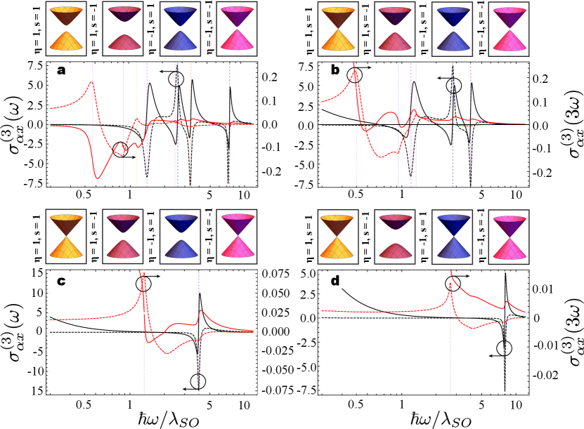
Next we show how one can identify signatures of the Chern numbers in each topological phase by investigating the nonlinear spectral response of the GFM. In Fig. 5 we present the frequency dispersion of the real part of the third-order optoelectronic longitudinal and transverse conductivities for both fundamental and third harmonics at four different points in phase space. These correspond to cases where all gaps are open (Fig. 5a) or one (Fig. 5b), two (Fig. 5c), or three (Fig. 5d) Dirac gaps are closed. The corresponding curves for the imaginary part (not shown) of the conductivities can be obtained directly from our formalism or via generalized Kramers-Kronig relations for nonlinear systems Hutchings1992 . We expect that the nonlinear conductivities should have non-negligible contributions when at least one Dirac gap matches one or three times the energy of the incident photons. Indeed, Fig. 5 shows that Kerr $\sigma_{\alpha x}^{(3)}(\omega)$ and third harmonic $\sigma_{\alpha x}^{(3)}(3\omega)$ conductivities present localized spectral resonances at $2\Delta_{s}^{\eta}=\hbar\omega$ (dashed vertical gridlines) and $2\Delta_{s}^{\eta}=3\hbar\omega$ (dotted vertical gridlines), respectively, with richer and more involved spectral responses in the cases where more Dirac cones are open. We mention that although the third-harmonic generation conductivity also includes resonances near $\omega$ and $2\omega$, they are difficult to identify in the spectrum because their magnitude are significantly smaller than the resonances near $3\omega$.

Note that near resonances the longitudinal Kerr and third harmonic conductivities always shows normal and anomalous dispersion, respectively, regardless of the resonant Dirac cone. This is due to the fact that both of these conductivities depend only on the absolute value of the resonant mass gap, hence not allowing to directly distinguish between energetically equivalent but topologically different points in the phase space. On the other hand, the transverse Hall conductivity is sensitive to the sign of the resonant $\Delta_{s}^{\eta}$ and, therefore, encodes information of the corresponding Pontryagin number ${\cal C}_{s}^{\eta}$. Note in Fig. 5, for instance, that $\sigma_{yx}^{(3)}(\omega)$ and $\sigma_{yx}^{(3)}(3\omega)$ have positive and negative resonances depending on the resonant Dirac gap. Therefore, just as the linear Hall conductivity allows to probe topological properties of the GFM at finite frequencies WiltonPRB , so it does at the nonlinear regime. Indeed, the Chern number associated to the open Dirac cones at any point in phase space can be computed by summing the sign of $\sigma_{yx}^{(3)}(\omega)$ or $\sigma_{yx}^{(3)}(3\omega)$ precisely at the resonant frequencies, accounting appropriately for degeneracy among mass gaps, and multiplying the result by $+1/2$ or $-1/2$, respectively. Consider, for example, the case in Fig. 5a. Note that in this case the third-order conductivity at the fundamental (third) harmonic evaluates to negative (positive) values in three of the four resonances. Thus, the sum of their signs equals $-2$ ($+2$) and results in a Chern number ${\cal C}=-1$, as expected for the PS-QHI phase in the $\lambda_{M}=0$ plane. Note that this argument can be extended to the nonlinear spin, valley, and spin-valley Hall currents, allowing for obtaining the full set of Chern numbers characterizing the topological phases in buckled two-dimensional semiconductors. In addition, unlike the linear case where to obtain the Chern number one needs to measure the linear Hall conductivity at various points around a resonance to obtain the sign of its derivative WiltonPRB , here we need to evaluate $\sigma_{yx}^{(3)}(3\omega)$ at most at the four (in the non-degenerate case) resonant frequencies. Finally, we mention that the dependence of the transverse (longitudinal) conductivities on $\textrm{sign}[\Delta_{s}^{\eta}]$ ($|\Delta_{s}^{\eta}|$) are not exclusive to the third order nonlinear case and similar conclusions should hold for higher order contributions as well.

Conclusions

In summary, we developed a comprehensive investigation of nonlinear light-matter interactions in spin-orbit coupled graphene materials, with focus on third harmonic generation and nonlinear corrections to the fundamental harmonic (Kerr effect). We have shown that by controlling various external parameters the monolayer can be driven through different phase transitions to explore the interplay between nonlinear effects and topological properties of two-dimensional materials. Specifically, we demonstrated that the helicity of the nonlinear scattered field encodes information about the location of the phase transitions boundaries, the dependence of the cross-polarized component of the field (proportional to the transverse conductivity) on the external parameters near resonances divulges details about the topological phases involved in the transition, and the dispersive nonlinear response of the system enables characterization of the Chern number in each phase. The recent progress in synthesis of topological semiconductors of the graphene family materials Silicene ; Germanene ; Stanene ; Plumbene and well established nonlinear characterization photonic techniques Kerr ; Gnonlinear2 ; Exp2 ; Exp3 ; Exp4 ; Exp5 suggest that our findings can be accessed experimentally with current technologies. We envision that the the effects predicted here will greatly impact research at the crossroads between nonlinear optics, topological materials, spintronics, and valleytronics.

Methods

In order to compute the nonlinear conductivity we need the unperturbed eigenvectors and the velocity matrix elements associated to the Hamiltonian in Eq. (1). In the following we will omit the valley and spin indexes $\eta$ and $s$ whenever possible, and the reader should keep in mind that, unless otherwise stated, all results presented are valid for a single Dirac cone. The total conductivities are given by summing the contributions of all mass gaps in the band structure. The eigenvector associated to the Hamiltonian in Eq. (1) has the form

$$|l\bm{k}\rangle=\frac{\hbar v_{F}|{\bf k}|}{\left[2\epsilon\left(\epsilon+l\Delta\right)\right]^{1/2}}\left(\begin{matrix}\frac{\epsilon+l\Delta}{\eta\hbar v_{F}|{\bf k}|}e^{-i\eta\theta}\\ l\end{matrix}\right),$$

(4)

where $|{\bf k}|=\sqrt{k_{x}^{2}+k_{y}^{2}}$, $\epsilon_{l}=l\epsilon=l\sqrt{\hbar^{2}v_{F}^{2}|{\bf k}|^{2}+\Delta^{2}}$, $l$ is the conduction ($l=+1$) and valence ($l=-1$) band index, and $\theta=\tan^{-1}(k_{y}/k_{x})$. The matrix elements $\langle l{\bf k}|\hat{v}_{\alpha}|l^{\prime}{\bf k}\rangle$ of the velocity operator $\hat{v}_{\alpha}=\hbar^{-1}\partial\hat{H}^{\eta}_{s}/\partial k_{\alpha}$ are given by

	$\displaystyle\langle 1\bm{k}|\hat{v}_{x}|-1\bm{k}\rangle$	$\displaystyle=$	$\displaystyle\langle-1\bm{k}|\hat{v}_{x}|1\bm{k}\rangle^{*}=-v_{F}\frac{\Delta\cos\theta+i\epsilon\sin\theta}{\epsilon},$		(5)
	$\displaystyle\langle 1\bm{k}|\hat{v}_{x}|1\bm{k}\rangle$	$\displaystyle=$	$\displaystyle-\langle-1\bm{k}|\hat{v}_{x}|-1\bm{k}\rangle=\frac{\hbar v_{F}^{2}k\cos\theta}{\epsilon},$		(6)
	$\displaystyle\langle 1\bm{k}|\hat{v}_{y}|-1\bm{k}\rangle$	$\displaystyle=$	$\displaystyle\langle-1\bm{k}|\hat{v}_{y}|1\bm{k}\rangle^{*}=-v_{F}\frac{i\epsilon\cos\theta-\Delta\sin\theta}{\epsilon},$		(7)
	$\displaystyle\langle 1\bm{k}|\hat{v}_{y}|1\bm{k}\rangle$	$\displaystyle=$	$\displaystyle-\langle-1\bm{k}|\hat{v}_{y}|-1\bm{k}\rangle=\frac{\hbar v_{F}^{2}k\sin\theta}{\epsilon}.$		(8)

We give a brief derivation for both the linear and third order optical conductivity terms for a particular Dirac cone. To this end, the equation of motion $i\hbar\partial\hat{\rho}(t)/\partial t=\left[{\hat{H}}_{s}^{\eta}+\hat{H}_{i}(t),\hat{\rho}(t)\right]$ for the density matrix operator is solved perturbatively by expanding the density matrix in powers of the potential vector amplitude ${\hat{\rho}}(t)=\sum_{n}{\hat{\rho}}^{(n)}(t)$ with ${\hat{\rho}}^{(n)}(t)\propto A^{n}$. To leading order in the potential vector, the first order density matrix upon Fourier transformation to the frequency domain can be cast as

$$\langle l{\bf k}|\rho^{(1)}(\omega)|l^{\prime}{\bf k}\rangle=\frac{-ieE_{\alpha}(\omega)}{\omega}\frac{f_{l^{\prime}{\bf k}}-f_{l{\bf k}}}{\epsilon_{l^{\prime}}-\epsilon_{l}+\hbar\omega}\langle l{\bf k}|\hat{v}_{\alpha}|l^{\prime}{\bf k}\rangle,$$

(9)

where $E_{\alpha}(\omega)=i\omega A_{\alpha}(\omega)/c$. Substituting $\hat{\rho}^{(1)}(\omega)$ in equation (2) and making use of the identity $[\hbar\omega\left(\epsilon_{l^{\prime}}-\epsilon_{l}+\hbar\omega\right)]^{-1}=[\epsilon_{l^{\prime}}-\epsilon_{l}]^{-1}[(\hbar\omega)^{-1}-(\epsilon_{l^{\prime}}-\epsilon_{l}+\hbar\omega)^{-1}]$, we eliminate the first term in the current $\propto Tr(\rho^{(0)})$ and re-obtain the well know Kubo formula after expressing the current as the product of conductivity and electric field

$$\sigma_{\alpha\beta}^{(1),\eta,s}(\omega)=-4i\hbar^{2}\sigma_{0}\sum\limits_{{\bf k},l,l^{\prime}}\frac{f_{l^{\prime}{\bf k}}-f_{l{\bf k}}}{\epsilon_{l^{\prime}}-\epsilon_{l}}\frac{\langle l{\bf k}|\hat{v}_{\beta}|l^{\prime}{\bf k}\rangle\langle l^{\prime}{\bf k}|\hat{v}_{\alpha}|l{\bf k}\rangle}{\epsilon_{l^{\prime}}-\epsilon_{l}+\hbar\omega},$$

(10)

where $\sigma_{0}=\alpha c/4$ and the phenomenological relaxation rate is accounted for by replacing $\omega\rightarrow\omega+i\Gamma$. Equation (10) accounts for both interband and intraband transitions. The interband contribution is straightforward and follows directly from (10) by setting $l^{\prime}\neq l$. The intraband contribution can be derived by equating enforcing $l^{\prime}=l$, in which case $(f_{l^{\prime}}-f_{l})/(\epsilon_{l^{\prime}}-\epsilon_{l})\rightarrow\partial f_{lk}/\partial\epsilon_{l}$. The total charge, spin, and valley linear conductivities are then computed as $\sigma_{\alpha x}^{(1)}(\omega)=\sum_{\eta,s}\sigma_{\alpha x}^{(1)\eta,s}(\omega)$, $\sigma_{\alpha x}^{(1),\textrm{s}}(\omega)=\sum_{\eta,s}s\sigma_{\alpha x}^{(1)\eta,s}(\omega)/2$, $\sigma_{\alpha x}^{(1),\eta}(\omega)=\sum_{\eta,s}\eta\sigma_{\alpha x}^{(1)\eta,s}(\omega)$, and $\sigma_{\alpha x}^{(1),s\eta}(\omega)=\sum_{\eta,s}s\eta\sigma_{\alpha x}^{(1)\eta,s}(\omega)/2$, respectively.

For the third order conductivities we first solve the equation of motion for third order correction $\rho^{(3)}(t)$, which is expressed in the Fourier space as

	$\displaystyle\langle l{\bf k}|\rho^{(3)}(\omega)|l^{\prime}{\bf k}\rangle=\frac{e^{3}E_{\alpha}(\omega_{1})E_{\beta}(\omega_{2})E_{\gamma}(\omega_{3})\!/\omega_{1}\omega_{2}\omega_{3}}{i\left(\epsilon_{l^{\prime}}-\epsilon_{l}+\hbar\omega_{1}+\hbar\omega_{2}+\hbar\omega_{3}\right)}\!\!\!\sum\limits_{l^{\prime\prime},l^{\prime\prime\prime}}$		$\displaystyle\!\!\frac{\langle l{\bf k}|\hat{v}_{\delta}\!|l^{\prime\prime\prime}{\bf k}\rangle\!\langle l^{\prime\prime\prime}{\bf k}|\hat{v}_{\gamma}\!|l^{\prime\prime}{\bf k}\rangle\!\langle l^{\prime\prime}{\bf k}|\hat{v}_{\beta}\!|l^{\prime}{\bf k}\rangle}{\epsilon_{l^{\prime}}-\epsilon_{l^{\prime\prime\prime}}+\hbar\omega_{1}+\hbar\omega_{2}}\!\!\left(\!\!\frac{f_{l^{\prime}{\bf k}}-f_{l^{\prime\prime}{\bf k}}}{\epsilon_{l^{\prime}}\!-\!\epsilon_{l^{\prime\prime}}\!+\!\hbar\omega_{1}\!}\!-\!\frac{f_{l^{\prime\prime}{\bf k}}-f_{l^{\prime\prime\prime}{\bf k}}}{\epsilon_{l^{\prime\prime}}\!-\!\epsilon_{l^{\prime\prime\prime}}\!+\!\hbar\omega_{2}}\!\right)$
			$\displaystyle\!\!\!\!\!\!\!\!-\frac{\langle l{\bf k}|\hat{v}_{\delta}\!|l^{\prime\prime\prime}{\bf k}\rangle\!\langle l^{\prime\prime\prime}{\bf k}|\hat{v}_{\gamma}\!|l^{\prime\prime}{\bf k}\rangle\!\langle l^{\prime\prime}{\bf k}|\hat{v}_{\beta}\!|l^{\prime}{\bf k}\rangle}{\epsilon_{l^{\prime\prime}}-\epsilon_{l}+\hbar\omega_{2}+\hbar\omega_{3}}\!\!\left(\!\!\frac{f_{l^{\prime\prime}{\bf k}}-f_{l^{\prime\prime\prime}{\bf k}}}{\epsilon_{l^{\prime\prime}}\!-\!\epsilon_{l^{\prime\prime\prime}}\!+\!\hbar\omega_{2}}\!-\!\frac{f_{l^{\prime\prime\prime}{\bf k}}-f_{l{\bf k}}}{\epsilon_{l^{\prime\prime\prime}}\!-\!\epsilon_{l}\!+\!\hbar\omega_{3}}\!\right).$

Substituting the above expression in Eq. (2) and using the same identity as before with the replacement $\omega\rightarrow\omega_{1}+\omega_{2}+\omega_{3}$, we obtain the third order optical conductivity per Dirac cone as

	$\displaystyle\!\!\!\!\!\!\!\!\sigma_{\alpha\beta\gamma\delta}^{(3)}(\omega_{1},\omega_{2},\omega_{3})$	$\displaystyle=$	$\displaystyle\dfrac{-e\hbar(\omega_{1}+\omega_{2}+\omega_{3})}{E_{\alpha}(\omega_{1})E_{\beta}(\omega_{2})E_{\gamma}(\omega_{3})}\times$		(13)
		$\displaystyle\times$	$\displaystyle\sum\limits_{{\bf k},l,l^{\prime}}\frac{\langle l{\bf k}|\hat{v}_{\alpha}|l^{\prime}{\bf k}\rangle}{\epsilon_{l^{\prime}}-\epsilon_{l}}\langle l^{\prime}{\bf k}|\rho^{(3)}(\omega)|l{\bf k}\rangle.$		(14)

The phenomenological relaxation rate can be accounted in a similar manner as in the linear case. Note that, Eq. (13) includes contributions from Berry connection, as well as intra and interband transitions Sipevelocity ; Aversa1995 . The nonlinear contributions to the fundamental harmonic associated to the Kerr effect follow by setting $\omega_{1}=\omega_{2}=-\omega_{3}$, while the third harmonic conductivity is can be derived for $\omega_{1}=\omega_{2}=\omega_{3}$. Similarly to the linear case the total charge, spin, valley, and spin-valley conductivities due to all Dirac cones are given by $\sigma_{\alpha x}^{(3)}(n\omega)=\sum_{\eta,s}\sigma_{\alpha x}^{(3)\eta,s}(n\omega)$, $\sigma_{\alpha x}^{(3),\textrm{s}}(n\omega)=\sum_{\eta,s}s\sigma_{\alpha x}^{(3)\eta,s}(n\omega)/2$, $\sigma_{\alpha x}^{(3),\eta}(n\omega)=\sum_{\eta,s}\eta\sigma_{\alpha x}^{(3)\eta,s}(n\omega)$, and $\sigma_{\alpha x}^{(3),s\eta}(n\omega)=\sum_{\eta,s}s\eta\sigma_{\alpha x}^{(3)\eta,s}(n\omega)/2$, respectively, where $n=1,3$.

Data availability

The data that support the plots within this paper and other findings of this study are available from the corresponding author on reasonable request.

Acknowledgements

Research presented in this article was supported by the Laboratory Directed Research and Development program of Los Alamos National Laboratory under project number 20190574ECR. The authors also thank the Center for Nonlinear Studies at LANL for financial support under project 20190495CR.

Author contributions

W.K.-K. proposed the study and developed the theory together with R.K.M. R.K.M. performed the numerical calculations. Both authors discussed the results and contributed to the final version of the manuscript. W.K.-K. supervised the entire study.

^∗ Corresponding author: kortkamp@lanl.gov

References

- [1] A. H. C. Neto, F. Guinea, N. M. R. Peres, K. S. Novoselov, A. K. Geim, The electronic properties of graphene. Rev. Mod. Phys. 81, 109 (2009).
- [2] N. M. R. Peres, Colloquium: The transport properties of graphene: An introduction. Rev. Mod. Phys. 82, 2673 (2010).
- [3] K. S. Novoselov, A. K. Geim, S. V. Morozov, D. Jiang, Y. Zhang, S. V. Dubonos, I. V. Grigorieva, and A. A. Firsov, Electric Field Effect in Atomically Thin Carbon Films, Science 306, 666 (2004).
- [4] M. Liu, X. Yin, E. Ulin-Avila, B. Geng, T. Zentgraf, L. Ju, F. Wang, and X. Zhang, A graphene-based broadband optical modulator, Nature 474, 64 (2011).
- [5] F. H. L. Koppens, D. E. Chang, and F. J. G. de Abajo, Graphene plasmonics: a platform for strong light-matter interactions, Nano Lett. 11, 3370 (2011).
- [6] K. S. Noveselov, A. K. Geim, S. V. Morozov, D. Jiang, M. I. Katsnelson, I. V. Grigorieva, S. V. Dubonos, and A. A. Firsov, Two-dimensional gas of massless Dirac fermions in graphene, Nature (London) 438, 197 (2005).
- [7] Y. Zhang, Y. -W. Tan, H. L. Stormer, and P. Kim, Experimental observation of the quantum Hall effect and Berry’s phase in graphene, Nature 438, 201 (2005).
- [8] N. M. R. Peres, F. Guinea, and A. H. Castro Neto, Electronic properties of disordered two-dimensional carbon. Phys. Rev. B 73, 125411 (2006).
- [9] S. Konschuh, M. Gmitra, and J. Fabian, Tight-binding theory of the spin-orbit coupling in graphene, Phys. Rev. B 82, 245412 (2010).
- [10] M. Z. Hasan and C. L. Kane, Colloquium: Topological insulators, Rev. Mod. Phys. 82, 3045 (2010).
- [11] X.-L. Qi and S.-C. Zhang, opological insulators and superconductors, Rev. Mod. Phys. 83, 1057 (2011).
- [12] P. Vogt, P. DePadova, C. Quaresima, J. Avila, E. Frantzeskakis, M. C. Asensio, A. Resta, B. Ealet, and G. Le Lay, Silicene: Compelling Experimental Evidence for Graphenelike Two-Dimensional Silicon, Phys. Rev. Lett. 108, 155501 (2012).
- [13] M. E. Dávila, L. Xian, S. Cahangirov, A. Rubio, and G. L.Lay, Germanene: a novel two-dimensional germanium allotrope akin to graphene and silicene, New J. Phys.16, 095002 (2014).
- [14] F. -f. Zhu, W. -j. Chen, Y. Xu, C. -l. Gao, D. -d. Guan, C. -h. Liu, D. Qian, S. -C. Zhang, and J. -f. Jia, Epitaxial growth of two-dimensional stanene, Nat. Mater. 14, 1020 (2015).
- [15] J. Yuhara, B. He, N. Matsunami, M. Nakatake, and G. Le Lay, Graphene’s latest cousin: Plumbene epitaxial growth on a ”Nano WaterCube”, Adv. Mater. 31, 1901017 (2019).
- [16] A. Castellanos-Gomez, Why all the fuss about 2D semiconductors?, Nat. Photonics 10, 202 (2016).
- [17] A. Molle, J. Goldberger, M. Houssa, Y. Xu, S.-C. Zhang,and D. Akinwande, Buckled two-dimensional Xene sheets, Nat. Mater. 16, 163 (2017).
- [18] A. J. Mannix, B. Kiraly, M. C. Hersam, and N. P. Guisinger, Synthesis and chemistry of elemental 2D materials, Nat. Rev. Chem. 1, 0014 (2017).
- [19] M. Ezawa, Monolayer Topological Insulators: Silicene, Germanene, and Stanene, J. Phys. Soc. Jpn. 84, 121003 (2015).
- [20] S. A. Mikhailov, Non-linear electromagnetic response of graphene, Europhys. Lett. 79, 27002 (2007);
- [21] S. A. Mikhailov and K. Ziegler, Nonlinear electromagnetic response of graphene: frequency multiplication and the self-consistent-field effects, J. Phys. Condens. Matter, 20, 384204 (2008).
- [22] K. F. Mak, C. Lee, J. Hone, J. Shan, and Tony F. Heinz, Atomically Thin MoS2: A New Direct-Gap Semiconductor, Phys. Rev. Lett. 105, 136805 (2010).
- [23] H. Zhang, S. Virally, Q. L. Bao, L. K. Ping, S. Massar, N. Godbout, and P. Kockaert, Z-scan measurement of the nonlinear refractive index of graphene , Opt. Lett. 37,1856 (2012).
- [24] E. Hendry, P. J. Hale, J. Moger, A. K. Savchenko, and S. A. Mikhailov, Coherent Nonlinear Optical Response of Graphene, Phys. Rev. Lett. 105, 097401 (2010).
- [25] J. J. Dean and H. M. van Driel, Graphene and few-layer graphite probed by second-harmonic generation: Theory and experiment, Phys. Rev. B 82, 125411 (2010).
- [26] R. Wu, Y. Zhang, S. Yan, F. Bian, W. Wang, X. Bai, X. Lu, J. Zhao, and E. Wang, Purely Coherent Nonlinear Optical Response in Solution Dispersions of Graphene Sheets, Nano Lett. 11, 5159 (2011)
- [27] N. Kumar, J. Kumar, C. Gerstenkorn, R. Wang, H. -Y. Chiu, A. L. Smirl, and H. Zhao, Third harmonic generation in graphene and few-layer graphite films, Phys. Rev. B 87, 121406(R) (2013).
- [28] S.-Y. Hong, J. I. Dadap, N. Petrone, P.-C. Yeh, J. Hone, and R. M. Osgood, Jr., Optical Third-Harmonic Generation in Graphene, Phys. Rev. X 3, 021014 (2013).
- [29] J. L. Cheng, N. Vermeulen, and J. E. Sipe, Third order optical nonlinearity of graphene, New J. Phys. 16, 053014 (2014).
- [30] J. L. Cheng, N. Vermeulen, and J. E. Sipe, Third-order nonlinearity of graphene: Effects of phenomenological relaxation and finite temperature, Phys. Rev. B 91, 235320 (2015).
- [31] F. Hipolito, T. G. Pedersen, and V. M. Pereira, Nonlinear photocurrents in two-dimensional systems based on graphene and boron nitride, Phys. Rev. B 94, 045434 (2016).
- [32] S. A. Mikhailov, Quantum theory of the third-order nonlinear electrodynamic effects of graphene, Phys. Rev. B 93, 085403 (2016).
- [33] A. Singh, K. I. Bolotin, S. Ghosh, and A. Agarwal, Nonlinear optical conductivity of a generic two-band system with application to doped and gapped graphene, Phys. Rev.B 95, 155421(2017).
- [34] M. Lysne, Y. Murakami, M. Schl̈er, and P. Werner. High-harmonic generation in spin-orbit coupled systems, Phys. Rev. B 102, 081121(R) (2020).
- [35] O. Zurrón, A. Picón, and L. Plaja. Theory of high-order harmonic generation for gapless graphene, New J. Phys. 20, 053033 (2018).
- [36] D. Bauer and K. K. Hansen, High-Harmonic Generation in Solids with and without Topological Edge States, Phys. Rev. Lett. 120, 177401 (2018).
- [37] C. Jürß and D. Bauer, High-harmonic generation in Su-Schrieffer-Heeger chains, Phys. Rev. B 99,195428 (2019).
- [38] R. Silva, A. Jiménez-Galán, B. Amorim, O. Smirnova and M. Ivanov. Topological strong-field physics on sub-laser-cycle timescale, Nat. Photon. 13, 849 (2019)
- [39] A. Chacón, W. Zhu, S. P. Kelly, A. Dauphin, E. Pisanty, A. Picón, C. Ticknor, M. F. Ciappina, A. Saxena, and M. Lewenstein, Circular dichroism in higher-order harmonic generation: Heralding topological phases and transitions in Chern insulators, Phys. Rev. B 102, 134115 (2020).
- [40] D. Baykusheva, A. Chacón, D. Kim, D. E. Kim, D. A. Reis, S. Ghimire, Strong-field physics in three-dimensional topological insulators, arXiv:2008.01265.
- [41] L. Stille, C. J. Tabert, and E. J. Nicol, Optical signatures of the tunable band gap and valley-spin coupling in silicene, Phys. Rev. B 86, 195405 (2012).
- [42] M. Ezawa, Photoinduced Topological Phase Transition and a Single Dirac-Cone State in Silicene, Phys. Rev. Lett. 110, 026603 (2013).
- [43] C. J. Tabert and E. J. Nicol, Dynamical polarization function, plasmons, and screening in silicene and other buckled honeycomb lattices. Phys. Rev. B 89, 195410 (2014).
- [44] P. Rodriguez-Lopez, W. J. M. Kort-Kamp, D. A. R. Dalvit, and L. M. Woods, Nonlocal optical response in topological phase transitions in the graphene family, Phys. Rev. Materials 2, 014003 (2018).
- [45] C. J. Tabert and E. J. Nicol, Valley-Spin Polarization in the Magneto-Optical Response of Silicene and Other Similar 2D Crystals, Phys. Rev. Lett. 110, 197402(2013).
- [46] P. Ledwith, and W. J. M. Kort-Kamp, and D. A. R Dalvit, Topological phase transitions and quantum Hall effect in the graphene family, Phys. Rev. B, 97, 165426 (2018).
- [47] P. Rodriguez-Lopez, W. J. M. Kort-Kamp, D. Dalvit, and L. M. Woods, Casimir force phase transitions in the graphene family, Nat. Commun.8, 14699 (2017).
- [48] M. B. Farias, W. J. M. Kort-Kamp, and D. A. R. Dalvit, Quantum friction in two-dimensional topological materials. Phys. Rev. B, 97, 161407(R) (2018).
- [49] W. J. M. Kort-Kamp, Topological phase transitions in the photonic spin Hall effect, Phys. Rev. Lett. 119,147401 (2017).
- [50] W. Wu, W. Zhang, S. Chen, X. Ling, W. Shu, H. Luo, S. Wen, and X. Yin, Optics Express 26, 23705 (2018).
- [51] W. Wu, S. Chen, W. Xu, Z. Liu, R. Lou, L. Shen, H. Luo, S. Wen, and X. Yin, Photonics Research 8, B47 (2020).
- [52] T. Kitagawa, T. Oka, A. Brataas, L. Fu, and E. Demler, Transport properties of nonequilibrium systems under the application of light: Photoinduced quantum Hall insulators without Landau levels, Phys. Rev. B 84, 235108 (2011).
- [53] M. Ezawa, Spin valleytronics in silicene: Quantum spin Hall-quantum anomalous Hall insulators and single-valley semimetals, Phys. Rev. B 87, 155415 (2013).
- [54] X. Li, T. Cao, Q. Niu, J. Shi, and J. Feng, Coupling the valley degree of freedom to antiferromagnetic order, Proc. Natl. Acad. Sci. USA 110, 3738 (2013).
- [55] Q.-F. Liang, L.-H. Wu, and X. Hu, Electrically tunable topological state in [111] perovskite materials with an antiferromagnetic exchange field, New J. Phys. 15, 063031(2013).
- [56] J. E. Sipe and E. Ghahramani, Nonlinear optical response of semiconductors in the independent-particle approximation, Phys. Rev. B 48, 11705 (1993).
- [57] C. Aversa and J. E. Sipe, Nonlinear optical susceptibilities of semiconductors: Results with a length-gauge analysis, Phys. Rev. B 52 , 14636 (1995).
- [58] A. Taghizadeh, F. Hipolito, and T. G. Pedersen, Linear and nonlinear optical response of crystals using length and velocity gauges: Effect of basis truncation, Phys. Rev. B 96, 195413 (2017).
- [59] D. C. Hutchings, M. Sheik-Bahae, D. J. Hagan, E. W. Van Stryland, Kramers-Krönig relations in nonlinear optics, Opt. Quant. Electron. 24, 1 (1992).