Nontrivial Topological Phases on the Stuffed Honeycomb Lattice
Abstract
We report the appearance of nontrivial topological phases in a tight-binding model on the stuffed honeycomb lattice. The model contains nearest neighbor and next nearest neighbor hopping terms coupled with an additional phase depending on the direction of hopping. Chern insulating and semi-metallic phases emerge with the change of hopping parameters. Nonzero Chern numbers characterizing the bands and the existence of topologically protected edge states in the gap between the relevant bands confirm the presence of those phases. We show that adding an extra basis to Haldane’s honeycomb model can lead to an additional topological phase characterized by Chern number . Transition between different topological phases driven by the hopping parameters has been illustrated in the topological phase diagram of the system. Zero temperature Hall conductivity along with density of states is evaluated. Topological properties of another tight-binding model on the stuffed square lattice are also reported in this article.
I Introduction
Investigation of nontrivial topological phases on various two-dimensional lattice models has been increasing rapidly in the recent times. These studies are motivated by the search of novel topological phases within new tight-binding models. These models are primarily characterized by a set of special energy bands those are separated by bulk energy gap but joined by quasi-continuous edge state energies. These are known as topological insulators (TI) which are distinguished by a topologically invariant integral number such as Chern number () TKNN , invariant, Kane1 etc.
It is established that the emergence of topological phases is the handiwork of specific phase factors which are incorporated into the tight-binding models through the hopping terms. In case of multipartite lattices, this phase factor appearing in the momentum space representation of the Hamiltonian is coupled with the hopping term between same or different sublattices. For instance, it arises in the one-dimensional bipartite Su-Schrieffer-Hegger model SSH only through the nearest neighbor (NN) hopping between two different sublattices. In this case, it depends on the Bloch wave vector, k. For the two-dimensional bipartite honeycomb lattice, an additional phase coupled with the next-nearest-neighbor (NNN) hopping between the same sublattice plays the crucial role to generate the nontrivial topological phases Haldane . Here, the sign of this phase is opposite for the two different sublattices. The net flux passing through a unit cell due to this gauge field is zero. The resulting Hamiltonians in these two cases break the Time Reversal Symmetry (TRS) due to the presence of this phase factor for which the topological energy bands are characterized by . In other words, this phase factor drives the system into an Integer Quantum Hall Effect (IQHE) regime.
On the other hand, topological phase appears in the honeycomb lattice due to the presence of spin-orbit coupling (SOC) for which the resulting Hamiltonian does not break the TRS Kane1 . Here, the system is characterized by invariant. However, if the Hamiltonian commutes with the -component of spin operator, , then the Hamiltonians for up and down spins break the TRS separately. In this case, resulting energy bands are characterized by spin-Chern numbers.
For a trivial insulator, the topological invariant is zero, while for a nontrivial TI, it can assume nonzero values. For example, there is nonzero for Chern insulators. Also, the number of edge states is proportional to the value of , which is known as the ‘bulk-boundary correspondence’ Hatsugai1 ; Hatsugai2 ; Kane2 . Due to this correspondence, the edge states which appear in a strip geometry become topologically protected. Thus, topological invariants are helpful for the classification of the topological phases of a system. A brief review on various TIs is available in the article Das .
Although the Chern insulating phase appears for TRS breaking Hamiltonians, the converse is not true. We cannot readily obtain nontrivial topological phase for all TRS breaking Hamiltonians. So, several attempts have been made in search of this phase in various multi-band systems. A number of two-dimensional lattices with nontrivial topological phase have been found and they are Lieb Franz , kagome Wen , checkerboard Das-sharma1 , square octagon Kargarian , diceWang ; Gong2 , star lattice Chen , etc. In addition, different topological flat-band models have also been proposed, where Fractional Quantum Hall Effect (FQHE) can be realized as those flat-bands carry nonzero Chern number Das-sharma2 .
Recently, nontrivial bands have been realized in optical lattices of ultracold atoms Wu by tuning the strengths of both NN and NNN hopping amplitudes Weiss and thus realization of artificial gauge field has been made possibleSpielman ; Aidelsburger . This has opened a new path of obtaining Chern insulator by varying the hopping parameters of the model tight-binding Hamiltonian in various two-dimensional lattice-systems Bergholtz ; Gong1 ; Beugeling .
In this work, we search for nontrivial topological phase on the stuffed honeycomb lattice, which is a three-band system by itself but actually interpolates the triangular (Bravais) and two-band honeycomb (non-Bravais) lattices. Being a two-band system honeycomb model is capable to exhibit nontrivial topological phase in the presence of phase-coupled hopping terms, while triangular lattice fails to do so under the same situation for obvious reason. Therefore, emergence of new topological phase in the interpolating regime will be of great interest. Eventually it turns out that addition of extra sublattice does lead to the emergence of new topological phase in the resulting system. In support of this claim, another tight-binding model on stuffed square lattice is hereby introduced which is capable to host new topological phase.
The antiferromagnetic (AFM) Heisenberg model on this lattice was studied previously in search of new spin-liquid phase. However, in that case, triangular, honeycomb as well as the intermediate stuffed honeycomb lattices were found to host similar kind of spin-liquid phase Sahoo . Interpolating lattices are capable to exhibit nontrivial spin chirality, which may lead to anomalous Hall Effect Nagaosa . S o, adding another basis to Haldane’s honeycomb model could provide the platform to explore novel topological phases in tight-binding regime. With this motivation, we formulated a three-band tight-binding model on this lattice in the presence of NN and NNN hopping terms. An additional phase coupled with NNN hopping has been considered to incorporate nontriviality in the otherwise trivial system. The sign of this phase depends on the direction of hopping. This phase breaks the TRS in the momentum space representation of the Hamiltonian. Also, the net flux of the gauge field passing through a unit cell is zero. The system is shown to exhibit distinct TI phases characterized by different sets of Chern numbers. Transition between those phases are driven by the modulation of hopping strengths. Chiral edge states are simultaneously obtained in the finite system.
The plan of the paper is as follows. In section II, stuffed honeycomb lattice is described and the tight-binding Hamiltonian is formulated. This is followed by section III, where behavior of the relevant physical quantities to study topological properties is presented. Finally, in section IV, discussions and conclusions on this work are summarized.
II Stuffed Honeycomb Lattice and Formulation of Hamiltonian
Stuffed honeycomb lattice originates as a result of coupling between one honeycomb lattice and one triangular lattice which is shown in Fig. 1(a). The honeycomb lattice is composed of two triangular lattices with site indices and , while the site index of the additional triangular lattice is . So, essentially it is tripartite and composed of three interpenetrating identical triangular lattices. The resulting lattice is decomposed in this manner to define the hopping parameters for this tight-binding model in a comfortable way. We consider three different species of spinless fermions each for three sublattices to introduce the Hamiltonian
| (1) | |||||
where is the site index. and indicate the summations over NN and NNN pairs. is the fermion creation operator at site . is the intra-honeycomb NN hopping amplitude and is the NN hopping amplitude between the honeycomb and triangular sublattices (Fig. 1(a)). is the NNN hopping amplitude irrespective of sublattices but = for solid (dashed) lines as shown in Fig. 1(b). The direction of the phases is indicated by the arrow in Fig. 1(b). is the onsite energy.
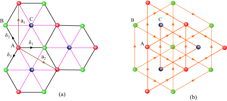
This model will become the honeycomb one when both and across the - bonds vanish. Similarly, it interpolates separately to triangular and dice lattices at = and at =, respectively Sahoo . The unit cell is defined by the primitive vectors and , where the NN distance is taken to be unity. NN sites are connected by the vectors and where and . All those vectors are shown in Fig. 1(a). The corresponding reciprocal lattice vectors are and which span the hexagonal first Brillouin zone.
Hamiltonian in the momentum space is written by invoking periodic boundary conditions along both and directions,
| (2) |
where , is a -component spinor and is a matrix. This can be expressed in terms of eight Gell-Mann matrices, as
| (3) |
with
| (4) | ||||
where is the identity matrix, , and . are shown in the Appendix A. We have written the Hamiltonian matrix in terms of and for ease of calculation. Evidently, TRS is broken by the phase since . Hopping parameters and as well as are measured with respect to which is taken as throughout the article. The value of is taken as () for honeycomb (triangular) sublattice. This special distribution of values of is necessary to open up gaps between the otherwise gapless energy bands.
Signs of hopping terms are taken in such a way that one among the three terms has sign opposite to that of the remaining two terms. This reverses the bloch phase of one of the off-diagonal elements of the Hamiltonian with respect to the other two (see Appendix A). We note that in the case of SU(3)-invariant models such a situation is a necessary criterion for generating the nontrivial topology Das2 .
Analytic expressions for the eigenvalues of are given by
| (5) |
; where the real parameters are
| (6) | ||||
Here, . The dispersion relations are shown in Fig. 2 (a) and (b) for two sets of where nonzero Chern numbers are found.
III Topological Properties
In order to study the topological properties, Chern numbers, Hall conductance at zero temperature and edge states of this model have been calculated.
III.1 Chern Numbers and Topological Phase Transition
In the beginning, we calculate of the three bands to characterize the topological phases of this system. is defined as the integration of the Berry curvature over the first Brillouin zone (1BZ), i.e.,
| (7) |
where . Here are the eigenvectors of and . is well-defined for a particular band as long as it does not touch other neighboring bands i.e., the eigenvalues are not degenerate for any fixed k. In our numerical calculation, we use the discretized version of Eq 7 introduced by Fukui and others Suzuki .
In this model, the presence of TRS breaking NNN phase, gives rise to the non-vanishing Chern number, since the TRS invariant Hamiltonian leads to resulting to . Evolution of both the dispersion relation and the topological phases is studied in a space spanned by the three parameters , and . does not change its sign if the sign of is reversed. However, is found to change its sign when either or changes its sign.
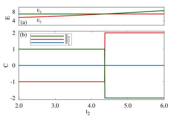
Let us now explain the evolution of topological phases along definite lines in this three-dimensional parameter space. At first, and are kept fixed at 6.0 and 2.0, respectively, while is allowed to vary. For , the two lower bands touch each other so that Chern numbers are ill-defined. As soon as becomes greater than , a pseudo-gap is opened up between the two lower bands and it remains so upto . This pseudo-gap becomes a true gap when . Along this line, there is always a true gap between the two upper bands as long as . Chern numbers are defined in these pseudo-gapped regions because of the fact that although the Fermi energy partially crosses one or more bands, no bands are found to touch each other. On the other hand, Fermi energy never crosses any band where true band gap exists. Pseudo-gapped phase is known as Chern semi-metallic phase, whereas the true gapped phase is known as Chern insulating phase. Thus, nontrivial topological phases appear over this line when , which is characterized by the value of . Two upper bands touch each other at where the system undergoes a topological phase transition. The closing of band gap at the transition point is essential to ensure the topological phase transition Kane2 . When , the Chern numbers are redistributed as . The Chern number exchange of may attribute to the fact that at , two upper bands touch each other simultaneously at three different points in the first Brillouin zone, say, , each causing an exchange of . No new topological phase is found to emerge upon further increase of , since no band crossing is observed.
In the same way, let us explore the evolution of topological phases along another line by keeping and fixed at and , respectively. At , the upper two bands touch each other and the Chern numbers are undefined. As soon as becomes nonzero, a nontrivial phase with appears but the system exhibits true band gaps upto . Afterwards, a pseudo gap develops between the two lower bands. This semi-metallic phase persists upto . For , the upper band-gap closes and the system becomes trivial. No new topological phase is found to appear further along this line.
Similarly, examining along many other lines in the parameter space, no new phase other than these two topologically different phases characterized by are found to exist. In every case, Chern number for the lowest band is zero. The phase diagram is presented in Fig 3 for and indicating transitions between different phases. It is evident that these topological phases are robust against change of external parameters as long as the alteration does not cause another band-touching or gap-closing.
The lowest energy band is partially localized on the triangular sublattice because of relatively strong sublattice potential, , with respect to that of honeycomb sublattice, . In the honeycomb limit, (i. e. and across C-C bond ), we get only a single phase, . Additional phase appears after turning on which results the stuffed honeycomb lattice. This fact may be termed as generation of additional topological phase due to the entry of an additional sublattice.
It would be worth mentioning in this context that a hard-core bosonic model based on this stuffed-honeycomb lattice has been studied before, where the topological phase with all topologically non-trivial bands ) is found. Additionally, the lowest band () bears high flatness ratio, 15, which gives rise to bosonic FQHE at 1/3 filling and fermionic FQHE at 1/5 filling Wang1 . On the other hand, in our fermionic model, although the lowest band becomes nearly flat when the values of both and are very small, the system is not a potential candidate for FQHE states as this band always carries zero Chern number. However, the topological phase () observed in the bosonic model could be realized in the fermionic counterpart by mimicking both the hopping terms and phase values like the former. As well as, FQHE state could be found in the lowest non-trivial flat band.
III.2 Hall conductance at zero temperature
At zero temperature, is estimated numerically by using the Kubo formula TKNN
where and . is the area of the system and is the Fermi energy. The velocity operator, , where . When falls in one of the energy gaps, the contribution to by completely filled bands is given by
| (8) |
In this situation, always assumes an integral value.
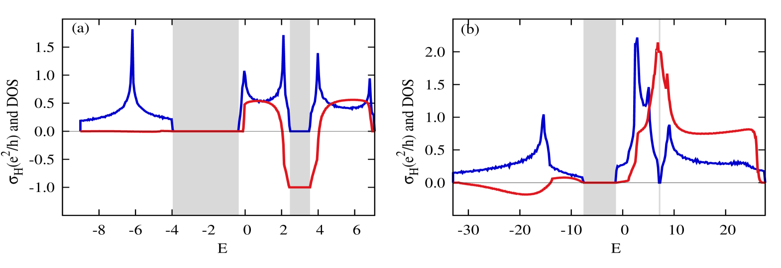
along with the density of states (DOS) is plotted against Fermi energy in Fig 4 for two different sets of parameters where two distinct topological phases are observed. DOS is useful to locate the gap in the band diagram where always exhibits a Hall plateau. The height of a Hall plateau can be determined by using Eq 8. Two prominent Hall plateaus for with are observed in Fig 4(a), which corresponds to the topological phase having . Similarly, in Fig 4(b) two Hall plateaus exist for with , but the second one is not prominent in the figure since the band gap is very narrow in this case. This characteristic corresponds to the topological phase having . Band gaps are identified by the shaded regions which hold these Hall plateaus. According to Eq 8, the value of over any Hall plateau becomes equal to the sum of all Chern numbers carried by the bands having energy lower than it. So, the sign of be either positive or negative depending on the distribution of over the energy bands. Also, width of the band gap equals to that of the plateau. DOS exhibits sharp peaks around the energies where undergoes sharp rise and fall. As a result, four sharp peaks in DOS are found in Fig 4(a). Another sharp peak in DOS at the lowest energy corresponds to the van Hove singularity in the band diagram.
III.3 Edge States
Among the topological properties, Chern number is recognized as the bulk property of the system, where edge states correspond to the surface property. However, the presence of non-zero Chern number leaves its signature by generating edge states, and vice versa. To study the properties of edge states in case of nontrivial Chern number, boundary lines or edges are created by removing the periodic boundary condition along axis, such that, is no longer a good quantum number for this finite system. But the periodic boundary condition along is there, so that acts as a good quantum number like before. The resulting strip has zigzag left and right edges.
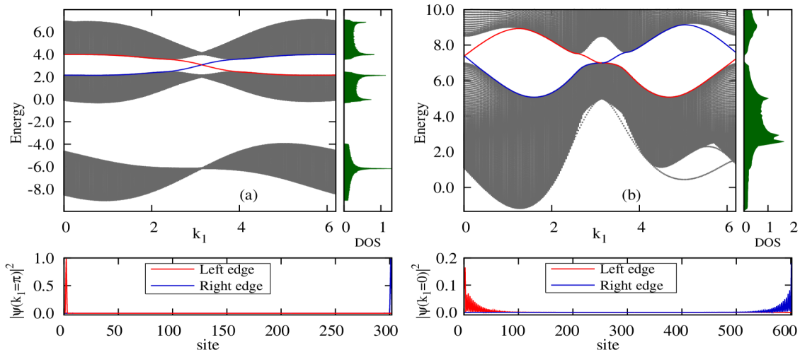
Here, a finite strip of stuffed Honeycomb lattice is considered which has cells, i.e., 300 sites along direction. The Hamiltonian has been constructed, which is a function of by taking partial Fourier transformation. Diagonalizing that Hamiltonian, the dispersion relation is obtained for , shown in Fig 5 (a), which reveals that the pattern of edge states supports the pattern of Chern numbers for the relevant topological phase of the system. Similarly, for other topological phase, , a honeycomb structure composed of cells along axis is considered. The dispersion relation for is shown in Fig 5 (b). To maintain a rich clarity in the figure, only two upper bands containing the edge states are shown in the second case. The edge states are indeed localized in either left (red curves) or right (blue curves) edge of the finite lattice, as shown in the lower panels of Fig 5. Chiral nature of these edge states are also confirmed from the figures, since the right-going (left-going) states are always localized in the right (left) edge.
As the lowest band always carries zero Chern number, no edge states are found to exist in the lower band gap for both phases. Two pairs of edge states are found in the upper band gap for , in contrast to one pair of that in the upper band gap for phase. Those results are in accordance with the ‘bulk-boundary correspondence’ rule which states that: sum of the Chern number upto the -th band, , is equal to the number of pair of edge states in the gap Mook . Thus the values of the Chern numbers can be recovered from the edge state pattern itself.
IV Summary and Discussion
A three-band tight-binding model on the stuffed honeycomb lattice has been proposed where an additional phase associated with the NNN hopping terms is found to break the TRS by yielding a Chern insulating phase in the presence of NN hopping. Although the same phase coupled with the NN hopping breaks TRS, it does not give rise to any nontrivial topological phase. The phase is chosen in such a way that the net flux of gauge field per unit cell vanishes. This system exhibits two different TI phases, Chern insulating and semi-metallic with nonzero Chern numbers in the parameter regimes. Also, this one undergoes quantum phase transition between two topological phases driven by the hopping parameters. Hall conductance exhibits prominent IQHE plateaus. The emergence of topologically protected chiral edge states in a strip configuration with open boundary condition is also found when .
This study reveals the fact that additional triangular sublattice leads to the generation of one additional topological phase in the resulting stuffed honeycomb lattice. It is established that topological phases could be induced within the trivial systems by means of introducing phase dependent hopping terms Haldane . So, more additional topological phases may be obtained by choosing those phases and hoppings in different ways. Topological phases with higher Chern numbers could be realized within a system by means of either exposing the systems to polarized light Arghya or invoking distant-neighbor hopping terms Piechon ; Moumita . Addition of extra sublattice may pave another route for the engineering of new topological phases wherever it is applicable. Thus, a desired topological phase may be realized in any system by combining those procedures along with the incorporation of additional sublattice. In this context, a tight-binding model is formulated on a body-centered stuffed square lattice which is found to harbour new topological phase. A brief description of the system as well as its topological properties is available in Appendix B.
The picture of stuffed honeycomb lattice is brought into light in the context of AFM compound, LiZn2Mo3O8 Flint . In this material the molecular cluster Mo3O8 forms a triangular lattice, however, its spin-liquid property is explained in terms of an effective spin-1/2 Heisenberg model built on the stuffed honeycomb lattice. Likewise, magnetic properties of the partially frustrated triangular AFM material, RbFeBr3, was explained before in terms of distorted triangular lattice, which is essentially the stuffed honeycomb lattice Adachi . However, no material is available at this moment where this electronic model could be realized for the verification of its topological properties.
V ACKNOWLEDGMENTS
AS acknowledges the CSIR fellowship, no. 09/096(0934) (2018), India. AKG acknowledges BRNS-sanctioned research project, no. 37(3)/14/16/2015, India.
Appendix A The Gell-Mann matrices
The Gell-Mann matrices are a set of eight traceless linearly independent Hermitian matrices spanning the Lie algebra of the SU(3) group. They are given below.
| (9) |
The off-diagonal upper triangular terms of are written as
| (10) | ||||
where
Appendix B Stuffed Square Lattice
In order to justify our claim that incorporation of additional sublattice may induce new topological phase, we consider the example of a particular stuffed square lattice. In this body-centered square lattice, a two-orbital (denoted by ) square sub-lattice incorporates another single-orbital (denoted by ) square sub-lattice in its centers which makes the system a three-band model, as shown in Fig. 6(a). However, in this case, the system is driven towards non-trivial topology phase as soon as the SOC between (1, 2) and 3 is invoked. The Hamiltonian of this tight binding model on this lattice can be written as
| (11) |
where
| (12) | |||||
| (13) | |||||
| (14) |
Here, is the NNN hopping parameter between sublattice 1 and 2 while is the NN hopping parameter between sublattice (1, 2) and 3. is the strength of SOC between NN pairs. The term , when the hopping takes place along (opposite to) the direction of the arrow as shown in fig 6(a). () is the annihilation (creation) operator of electron at site , such that , where, () is the annihilation operator of the electron with up (down) spin. for the horizontal (vertical) NNN bond.
After applying Fourier transformation, the resulting Hamiltonian, , comprises two uncoupled diagonal blocks corresponding to up and down spins, those are related by time-reversal symmetry, i. e., . Now it is sufficient to consider either up- or down-spin sector for the calculation of energy spectrum and topological properties. It is noted that, the up- and down-spin sectors break TRS separately. So, we can treat Chern number as the topological invariant following the previous formulation as described in the main text. If we denote the Chern number for -th band for up-spin sector as and down-spin sector as , then and spin Chern number for the whole -th band can be defined as . In the following, we restrict to the spin up sector only and omit the spin symbol for convenience. So,
| (15) |
where and is a three-component spinor. can be expressed as
| (16) |
with
| (17) | ||||
When , the three bands touch each other and so the Chern numbers are ill-defined. As soon as becomes non-zero, gaps open up between the bands and this time those bands are characterized by definite Chern numbers, . Fig. 6 (b) shows the band structure for , and .
For the calculation of edge states, we consider a finite strip of stuffed square lattice consisting of 100 cells i. e., 300 sites along -direction. By diagonilizing the resulting Hamiltonian as a function of good quantum number , the dispersion of edge states is obtained, which is shown in Fig. 6(c). Two pair of edge states are found in both the band-gaps, which is in accordance with the ‘bulk-boundary correspondence’ rule. DOS is shown in the side panel of the associated figure. Therefore, we put forward another example through which we successfully demonstrate the emergence of new topological phase with the addition of extra sublattice where the tight-bindig model on the parent lattice was topologically trivial.
References
- (1) Thouless D. J., Kohomoto M., Nightingale P. and den Nijs M., Phys. Rev. Lett. 49, 405 (1982).
- (2) Kane C. L. and Mele E. J., Phys. Rev. Lett. 95, 146802 (2005).
- (3) Heeger A. J., Kivelson S., Schrieffer J. R. and Su W. P., Rev. Mod. Phys. 60, 781 (1988).
- (4) Haldane F. D. M., Phys. Rev. Lett. 61, 2015 (1988).
- (5) Hatsugai Y., Phys. Rev. Lett. 71, 3697 (1993).
- (6) Hatsugai Y., Phys. Rev. B 48, 11851 (1993).
- (7) Hasan M. Z. and Kane C. L., Rev. Mod. Phys. 82, 3045 (2010).
- (8) Das T. A, arXiv:1604.07546
- (9) Weeks C. and Franz M., Phys. Rev. B 82, 085310 (2010).
- (10) Tang E., Mei J. W. and Wen X. G., Phys. Rev. Lett. 106, 236802 (2011).
- (11) Sun K., Gu Z., Katsura H. and Das Sarma S., Phys. Rev. Lett. 106, 236803 (2011).
- (12) Kargarian M. and Fiete G. A., Phys. Rev. B 82, 085106 (2010).
- (13) Liu X.P., Chen W. C., Wang Y. F. and Gong C. D., J. Phys.: Condens. Matter 25, 305602 (2013).
- (14) Wang F. and Ran Y., Phys. Rev. B 84, 241103(R) (2011).
- (15) Chen W. C., Liu R., Wang Y. F. and Gong C. D., Phys. Rev. B 86, 085311 (2012).
- (16) Yang S., Gu Z., Sun K. and Das Sarma S., Phys. Rev. B 86, 241112(R) (2012).
- (17) Wu C., Phys. Rev. Lett. 101, 186807 (2008).
- (18) Eckardt A., Weiss C. and Holthaus M., Phys. Rev. Lett. 95, 260404 (2005).
- (19) Jiménez-García K. et. al., Phys. Rev. Lett. 108, 225303 (2012).
- (20) Aidelsburger M. et. al., Nature Phys. 11, 162 (2015).
- (21) Trescher M. and Bergholtz E. J., Phys. Rev. B 86, 241111(R) (2012).
- (22) Liu R., Chen W.C., Wang Y. F. and Gong C. D., J. Phys.: Condens. Matter 24, 305602 (2012).
- (23) Beugeling W., Everts J. C. and Morais Smith C., Phys. Rev. B 86, 195129 (2012).
- (24) Sahoo J., Kochkov D., Clark B. K. and Flint R., Phys. Rev. B 98, 134419 (2018).
- (25) Nagaosa N. et. al., Rev. Mod. Phys. 82, 1539 (2010).
- (26) Ray S., Ghatak A. and Das T., Phys. Rev. B 95, 165425 (2017).
- (27) Fukui T., Hatsugai Y. and Suzuki H., J. Phys. Soc. Jpn. 74, 1674 (2005).
- (28) Wang Y-F., Hong Y., Gong C-D., and Sheng D. N., Phys. Rev. B 86, 201101(R) (2012).
- (29) Mook A., Henk J. and Mertig I., Phys. Rev. B 90, 024412 (2014).
- (30) Sil A. and Ghosh A. K., J. Phys.: Condens. Matter 31, 245601 (2019).
- (31) Sticlet D. and Piéchon F., Phys. Rev. B 87, 115402 (2013).
- (32) Deb M. and Ghosh A. K., J. Phys.: Condens. Matter 31, 345601 (2019).
- (33) Flint R. and Lee P. A., Phys. Rev. Lett. 111, 217201 (2013).
- (34) Adachi K. et al., J. Phys. Soc. Jpn. 52, 2202 (1983).