Normal approximation for fire incident simulation using permanental Cox processes

A point process is a collection of random points on some mathematical space, such as Euclidean space $\mathbb{R}^{d}$. As mentioned earlier, point processes are popular tools in the insurance industry (see [2], [27] and [30]).

Let $X\subset\mathbb{R}^{d}$ with $d\in\mathbb{N}$ be a point process. For $\text{card}(A)$, the cardinality of $A\subset\mathbb{R}^{d}$, let

The point process $X$ is said to be simple if $N(\{{\bf a}\})\in\{0,1\}$ a.s. for all ${\bf a}\in\mathbb{R}^{d}$. Also, the process $X$ is said to be locally finite if it takes values in

The process $X$ is said to be negatively associated if for all coordinate-wise increasing functions $\psi:\mathbb{N}^{k}\rightarrow\mathbb{R}$ and $\phi:\mathbb{N}^{l}\rightarrow\mathbb{R}$ and for all families of pairwise disjoint Borel sets $\{A_{i}\mid 1\leq i\leq k\}$ and $\{B_{j}\mid 1\leq j\leq l\}$ such that

we have

Similarly, the point process is said to be positively associated if the above inequality is reversed and the families of Borel sets are not necessarily assumed to satisfy (1). In addition, a point process is said to be associated if it is either negatively or positively associated.

Next, we state the definition of the nth order intensity functions of point processes with respect to Lebesgue measure. Let $n\in\mathbb{N}$ and $X\in\Omega$. If there exists a non-negative function $\rho_{n}:\left(\mathbb{R}^{d}\right)^{n}\rightarrow\mathbb{R}$ such that

for all locally integrable functions $f:\left(\mathbb{R}^{d}\right)^{n}\rightarrow\mathbb{R}$, then $\rho_{n}$ is called the nth order intensity function of $X$. Now, for ${\bf x},{\bf y}\in\mathbb{R}^{d}$, let

It follows that

Cox processes are well-known point processes. They are considered to be generalizations of the Poisson point processes for which the intensity is a random measure. A permanental Cox process [19] is the Cox process with intensity functions

where $\Lambda$ is a random measure defined as

where the $Y_{1},\ldots,Y_{l}$ are $l$ independent, zero-mean, real-valued Gaussian random fields with covariance function $C$.

In this work, we consider the case where the Gaussian random fields are stationary; hence, $C$ only depends on $r=|{\bf x}_{i}-{\bf x}_{j}|_{\infty}$, where $|\cdot|_{\infty}$ denotes the vector max norm. Also, we consider just the specific case when

where $\kappa_{c}$ and $\lambda_{c}$ are constants. This process has been used, for instance, in [20], [31] and [21]. It is known to be positively associated (see [11] and [18]).

Stein’s method, introduced by Charles Stein [26] in 1972, is a widely known technique for finding non-asymptotic bounds for approximations of probability distributions. It was motivated by the idea that $W$ has the standard Normal distribution if and only if

for all absolutely continuous functions $f$ with $\mathbb{E}|f^{\prime}(W)|<\infty$. This identity leads to the differential equation

where $Z$ is a standard Normal random variable and $h$ is a test function. If $h\in\mathcal{H}$ for some Borel set $\mathcal{H}$ and we replace $w$ by a random variable $W$, the error in the distributional approximation of $W$ by $Z$ on $\mathcal{H}$ can be bounded by obtaining the non-asymptotic bound of the expectation of the supremum of the right-hand side of (6) over $\mathcal{H}$. In general, doing so is much simpler than computing the left-hand side of (6) directly. Taking $h\in\mathcal{H}_{1}$, where $\mathcal{H}_{1}=\{h\mid|h(x)-h(y)|\leq|x-y|\}$, we obtain

This distance is known as $L^{1}$ or the Wasserstein distance. Stein’s method has been used in various applications, and it is one of the best ways to handle dependent situations (see [6] and [24]). One of the classic dependent cases, handled by Stein’s method, is the local dependent structure introduced in [7]. A collection of random variable $X_{1},\ldots,X_{n}$ has dependency neighborhoods $N_{i}\subseteq\{1,2,\ldots,n\},i=1,2,\ldots,n$ if $X_{i}$ is independent of $X_{j}$ for all $j\notin N_{i}-\{i\}$. Next, we state a version of the local dependence bound that appeared in the note [24].

We apply Theorem 2.1 to obtain our main results in the next section.

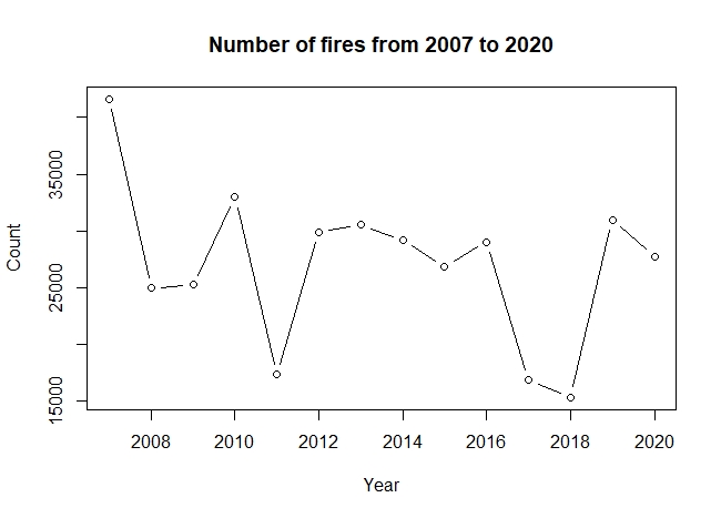
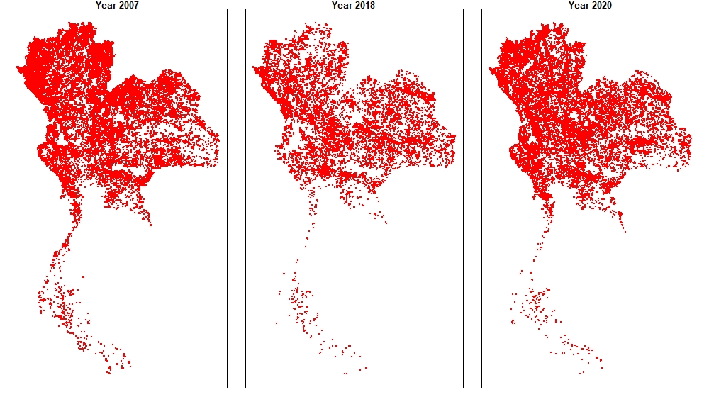
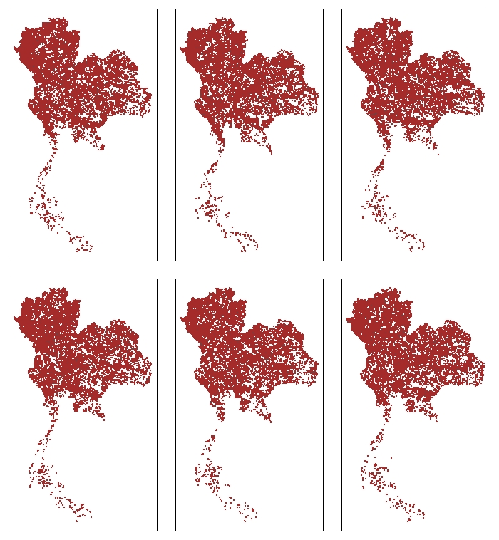
In this subsection, we first explore the dataset and verify that it does not contradict the assumptions in Theorem 3.3. We follow the process outlined in Figure 1. Figure 2 shows the total number of fires each year in Thailand, where the mean and the standard deviation were 27,048 and 6,980.94, respectively. Figure 3 shows the locations of fires in 2007, 2014 and 2020, respectively, from left to right.

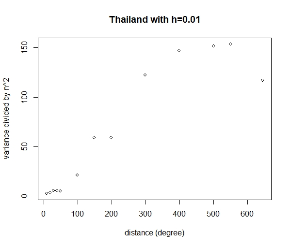
We now examine whether the fire dataset follows assumptions (12) and (13). As the actual intensity function is unknown and cannot be obtained from the dataset, we can only check the covariances between fire counts in two distinct areas separated by a distance $r$. We first check to see if the covariance does not decay in a small local neighborhood. Then we further check to see if the covariance decays exponentially as the distance between areas increases. We also show the variances of the fire counts corresponding to $n$, with $n$ going from 10 to 645, where $645$ is the greatest distance possible in Thailand (1 unit equals to 0.01 degrees of latitude or longitude). Note that the total area of Thailand is 513,120 square kilometers, which equals $716^{2}$. Since 1 degree is about 111 kilometers, the total area is approximately $6.45^{2}$ square degrees, which is equivalent to $645^{2}$ square units when 1 unit is 0.01 degrees. Therefore, the largest $n$ possible in Thailand is 645.

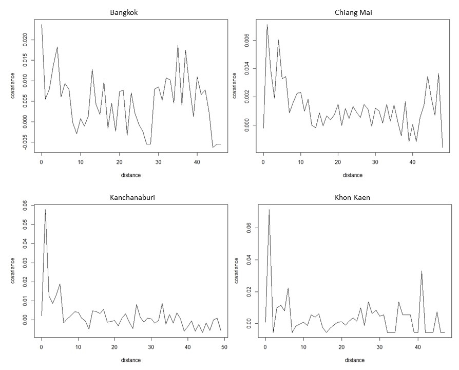
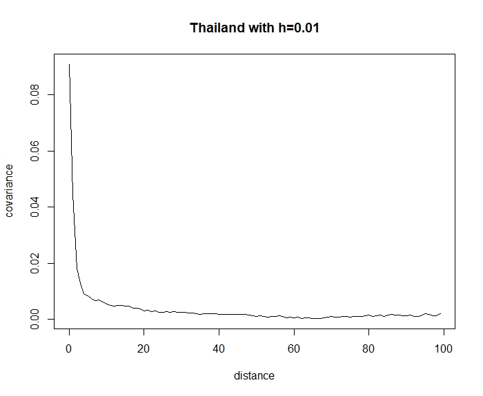
As the entire country is too large to be considered a small local neighborhood, we specifically check four provinces from four regions, including Bangkok, Chaing Mai, Kanchanaburi and Khon Kaen. Note that we did not select a province from Southern Thailand, as the number of fires in this region was too low. Figure 4 shows no sign of exponential decay in the covariance pattern for these provinces when the unit distance is 0.002 degrees ($\sim 222$ meters). Figure 5 shows the covariance decay pattern based on distance for all of Thailand. We obtain an exponential decay rate of 0.15 when we use a unit distance of 0.01 degrees ($\sim 1.11$ kilometers). Figure 6 shows the values of $\sigma_{n}^{2}/n^{2}$ for $n$ from 10 to 645. Obviously, assumption 13 is not contradicted.

We devote this subsection to simulating fires in Thailand via the process outlined in Figure 7.

We first model Thailand’s fires using permanental Cox processes. Note that when we refer to the area ${\bf x}$, we are referring to a unit square that has ${\bf x}$ at the top left corner, where ${\bf x}\subset\mathbb{R}^{2}$ and 1 unit equals 0.01 degrees of latitude or longitude. We estimate the variances of $Y_{j}({\bf x}_{i})$ and $l$ from

by using the first two sample moments. We set the means of the data and process to be equal and seek the closest variances. Writing $\sigma_{j}^{2}({\bf x}_{i})=\mathrm{Var}(Y_{j}({\bf x}_{i}))$ for each ${\bf x}_{i}$ and using the fact that the $Y_{j}({\bf x}_{i})$ for $j=1,2,\ldots,l$ are zero-mean, independent Gaussian random variables, we set $\sum_{j=1}^{l}\sigma_{j}^{2}({\bf x}_{i})$ equal to the sample mean of area ${\bf x}_{i}$ and $2\sum_{j=1}^{l}\sigma_{j}^{4}({\bf x}_{i})$ equal to the sample variance of area ${\bf x}_{i}$. We then set $\sigma_{j}^{2}({\bf x}_{i})=\sigma^{2}({\bf x}_{i})$ for all $j$ for simplicity and solve for the closest $\sigma^{2}({\bf x}_{i})$ and $l$.

Denoting $m({\bf x}_{i})$ and $v({\bf x}_{i})$ as the mean and variance of the total fires in the unit cube at position ${\bf x}_{i}$ from the dataset, we have

Then setting

and substituting $\sigma^{2}({\bf x}_{i})$, we have

For simplicity, we set $l=\max\left(1,\left\lfloor\frac{2m^{2}({\bf x}_{i})}{v({\bf x}_{i})}\right\rfloor\right)$. Although the $l$’s differ for different ${\bf x}_{i}$, we can choose the largest $l$. For a ${\bf x}_{i}$ with a smaller $l$, we set $\sigma^{2}({\bf x}_{i})$ equal to zero for all the remaining terms.

To estimate the covariance function of the Gaussian processes from (5), we need estimates of $\kappa_{c}$ and $\lambda_{c}$. Plugging in $r=0$, we have $\kappa_{c}=\sigma^{2}({\bf x}_{i})$; thus, it suffices to estimate $\lambda_{c}$. We seek a $\lambda_{c}$ from a fine grid from 0 to 0.5 that results in the covariance decay rate closest to the 0.15 from the real dataset. Note that the decay rate of 0.15 is computed from the number of fires, whereas $\lambda_{c}$ is the decay rate of the covariance function for the Gaussian process. Therefore, it is not possible to set $\lambda_{c}=0.15$ directly.

By following the procedure above, we find the largest $l$, i.e., $l=8$, and closest $\lambda_{c}(0.1$). Figure 8 shows an example of a simulation with parameters estimated from the procedure above and 6 iterations.

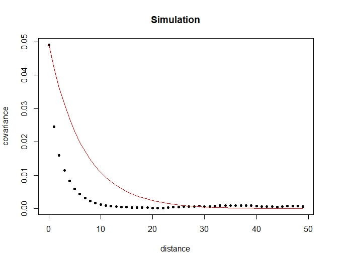
Next, we simulate fire counts for the whole country for 20 iterations and check that the covariance decays exponentially with distance. Since the number of areas in the entire country at a unit distance of 0.01 degrees from another area is extremely large, 20 is a reasonable number of iterations for the simulation. Figure 9 shows the covariance plot and the decay rate of 0.15 from the real dataset.

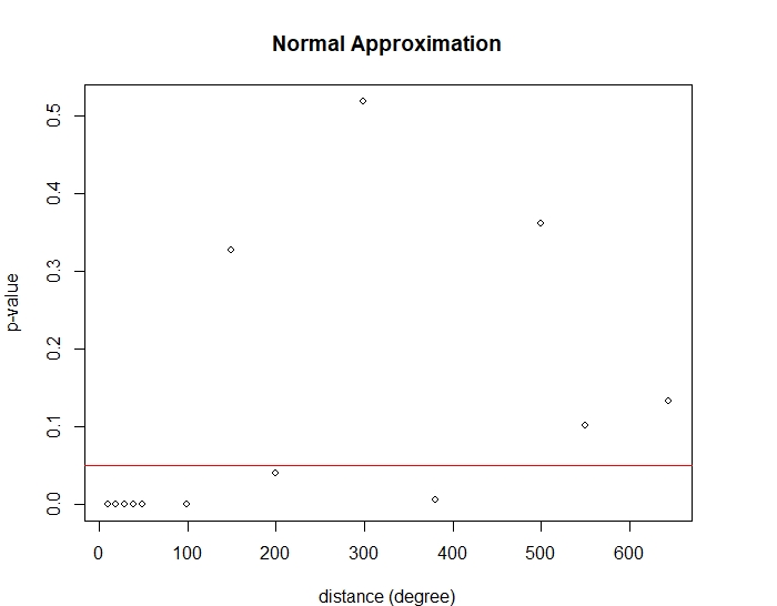
Then we simulate fires across the whole country for 500 iterations to check that the variance is on the order of $n^{2}$ and to compare the results with the Normal approximation from Theorem 3.3. As in Subsection 4.1, we take $n$ from 10 to 645, where $645$ units is the greatest distance possible in Thailand (1 unit equals 0.01 degrees of latitude or longitude). We preliminarily check the normality of the simulated fire counts using the Shapiro–Wilk test. Figure 10 shows the Shapiro–Wilk p-values based on $n$, while the red horizontal line indicates the 0.05 significance level. We can see that when $n$ is large, the null hypothesis that the total number of fires is Normally distributed is not rejected.

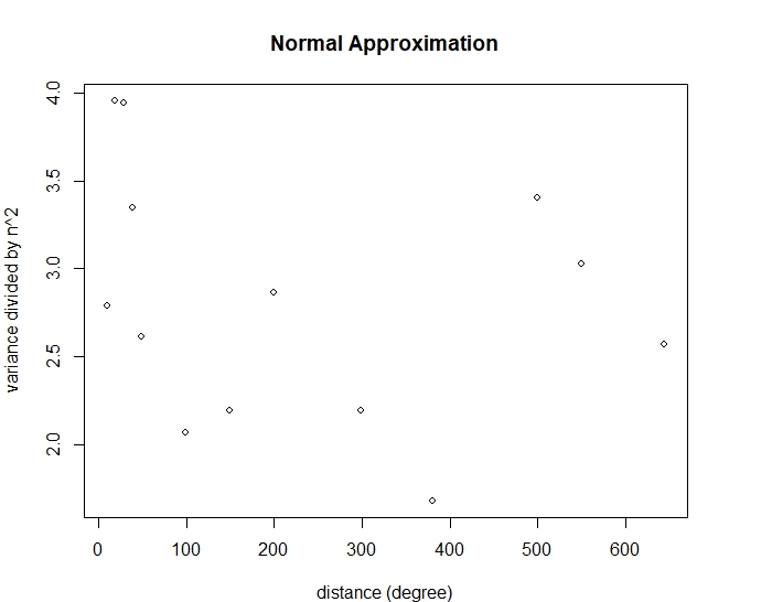
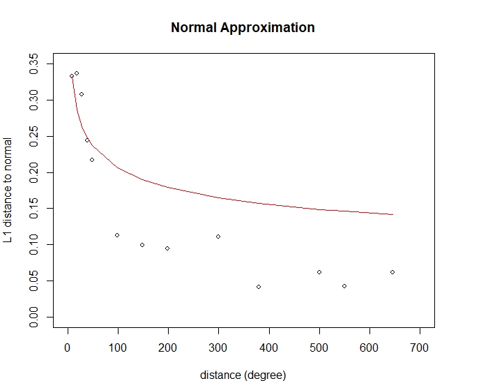
We end this section by checking the variance assumption in assumption (13) and compare the simulation’s $L^{1}$ distance to the bound in (14). Figure 11 shows a random pattern for the variances of fire counts divided by $n^{2}$, which agrees with assumption (13). Figure 12 shows the $L^{1}$ distances between the standardized fire counts from our simulation and a standard Normal distribution . We also plot the rate of convergence of $n^{d/(4d+2)}$ from Theorem 3.3. The rate from our simulation tends to follow the rate from our main bound.

The main assumptions that we made in this work is that the fire counts for two distinct areas are positively associated and their covariance decays exponentially with respect to their distance from each other. Nevertheless, the decay rate may vary from country to country or area to area and may also change over time. Therefore, in this section, we are interested in examining the Normal approximation results for different covariance decay rates through the parameter $\lambda_{c}$ from (5).

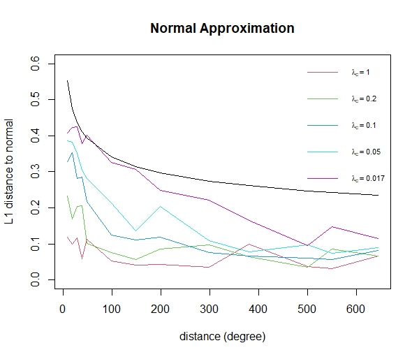
Figure 13 shows that the $L^{1}$ distances between the standardized fire counts from our simulation and a standard Normal distribution for areas ranging in size from 9 to 645 square degrees when $\lambda_{c}=1,0.2,0.1,0.05,0.017$. The black line shows the rate of convergence of $n^{d/(4d+2)}$ from Theorem 3.3. Intuitively, the distribution should be closer to the Normal distribution when $\lambda_{c}$ is larger, as a larger value implies that the fire counts in the areas are closer to independence. This reasoning agrees with the simulation results shown in Figure 13.

References

- [1] Abledu, G. K., Dadey, E. and Kobina , A., Probability modeling and simulation of insurance claims in Ghana, Global Journal of Commerce & Management Perspective, 3(5) (2014) 41–49.
- [2] Albrecher, H., Araujo-Acuna, J. C. and Beirlant, J., Fitting non-stationary Cox process: an application to fire insurance data, North American Actuarial Journal, 0(0) (2020) 1–28.
- [3] Barbour, A. D., Stein’s method and Poisson process convergence, Journal of Applied Probability, 25 (1988) 175–184.
- [4] Barbour, A. D. and Brown, T. C., Stein’s method and point process approximation, Stochastic Processes and their Applications, 43(1) (1992) 9–31.
- [5] Bärtl, M. and Krummaker, S., Prediction of claims in export credit finance: a comparison of four machine learning techniques, Risks, 8(22) (2020) 1–29.
- [6] Chen, L.Y.H., Goldstein, L. and Shao, Q.M., Normal Approximation by Stein’s Method, Springer, New York, 2011.
- [7] Chen, L.Y.H. and Shao, Q.M., Normal approximation under local dependence, Annals of Probability, 32 (2004) 1985–2028.
- [8] Chen, L.Y.H. and Xia, A., Stein’s method, Palm theory and Poisson process approximation, Annals of Probability, 32(3) (2004) 2545–2569.
- [9] Chen, L.Y.H. and Xia, A., Poisson process approximation: from Palm theory to Stein’s method, IMS Lecture Notes-Monograph Series: Time Series and Related Topics, 52 (2006) 236–244.
- [10] Chen, L.Y.H. and Xia, A., Poisson process approximation for dependent superposition of point processes, Bernoulli, 17(2) (2011) 530–544.
- [11] Eisenbaum, N., Characterization of positively correlated squared Gaussian processes, The Annals of Probability, 42(2) (2014) 559–575.
- [12] Gabrielli, A. and Wüthrich, M. V., An individual claims history simulation machine, Risks, 6(29) (2018) 1–33.
- [13] Heffernan, J.E. and Resnick, S.I., Limit laws for random vectors with an extreme component, Annals of Applied Probability, 17 (2007) 537–571.
- [14] Jessen A.H., Mikosch T. and Samorodnitsky G., Prediction of outstanding payments in a Poisson cluster model, Scandinavian Actuarial Journal, 3(2011) 214–237.
- [15] Keef, C., Svensson C. and Tawn, J.A., Spatial dependence in extreme river flows and precipitation for Great Britain, Journal of Hydrology, 378 (2009) 240–252.
- [16] Keef, C., Tawn, J. A. and Lamb, R., Estimating the probability of widespread flood events, Environmetrics, 24 (2013) 13–21.
- [17] Lamb, R., Rainfall-runoff modelling for flood frequency estimation, Encyclopedia of Hydrological Sciences, Anderson MG (eds). John Wiley & Sons(2005) 1923–1954.
- [18] Last, G., Szekli, R., Yogeshwaran, D., Some remarks on associated random fields, random measures and point processes, ALEA Latin American Journal of Probability and Mathematical Statistics, 17 (2020) 355–374.
- [19] McCullagh, P., Møller, J., The permanental process, Advances in Applied Probability, 38(4) (2006) 873–888.
- [20] McCullagh, P., Yang, J., Stochastic classification models, International Congress of Mathematicians, 3 (2006) 669–686.
- [21] Mustafa, H. A., Ekti, A. R., Shakir, M. Z., Imran, M. A., Tafazolli, R., Intracell interference characterization and cluster interference for D2D communication, IEEE Transactions on Vehicular Technology, 67(9) (2018) 8536–8548.
- [22] Poinas, A., Delyon, B. and Lavancier, F., Mixing properties and central limit theorem for associated point processes, Bernoulli, 25(3) (2019) 1724–1754.
- [23] Quan, Z. and Valdez, E.A., Predictive analytics of insurance claims using multivariate decision trees, Dependence Modeling, 6 (2018) 377–407.
- [24] Ross, N. Fundamentals of Stein’s method. Probability Surveys, 8 (2011) 210–293.
- [25] Schoenberg, F.P., Chang, C., Keeley, J., Pompa, J., Woods, J. and Xu, H., A critical assessment of the burning index in Los Angeles County, California, International Journal of Wildland Fire, 16(4) (2007) 473–483.
- [26] Stein, C., A bound for the error in the normal approximation to the distribution of a sum of dependent random variables. Proceedings of the Sixth Berkeley Symposium on Mathematical Statistics and Probability University of California Press, 2 (1972) 210–293.
- [27] Törnqvist, G., Modelling insurance claims with spatial point process: an applied case-control study to improve the use of geographical information in insurance pricing, Master thesis, Umeå University, 2015
- [28] Wiroonsri, N., Normal approximation for associated point processes via Stein’s method with applications to determinantal point processes, Journal of Mathematical Analysis and Applications, 480(1) (2019) 123396.
- [29] Wüthrich M. V., Machine learning in individual claims reserving, Scandinavian Actuarial Journal, (2018) 1–16.
- [30] Xu, H. and Schoenberg F.P., Point process modeling of wildfire hazard in Los Angeles County, California, The Annals of Applied Statistics, 5(2011) 684–704.
- [31] Yang, J., Miescke, K., McCullagh, P., Classification based on a permanental process with cyclic approximation, Biometrika, 99(4) (2012) 775–786.