Normal/inverse Doppler effect of backward volume magnetostatic spin waves
Abstract
Spin waves (SWs) and their quanta, magnons, play a crucial role in enabling low-power information transfer in future spintronic devices. In backward volume magnetostatic spin waves (BVMSWs), the dispersion relation shows a negative group velocity at low wave numbers due to dipole-dipole interactions and a positive group velocity at high wave numbers, driven by exchange interactions. This duality complicates the analysis of intrinsic interactions by obscuring the clear identification of wave vectors. Here, we offer an innovative approach to distinguish between spin waves with varying wave vectors more effectively by the normal/inverse spin wave Doppler effect. The spin waves at low wave numbers display an inverse Doppler effect because their phase and group velocities are anti-parallel. Conversely, at high wave numbers, a normal Doppler effect occurs due to the parallel alignment of phase and group velocities. Analyzing the spin wave Doppler effect is essential for understanding intrinsic interactions and can also help mitigate serious interference issues in the design of spin logic circuits.
The concept of spin waves (SWs), initially introduced by F. Bloch in 1932, was expanded upon in the 1940s by Holstein & Primakoff and Dyson. They described SWs as wave-like excitations in magnetic materials, propagated through exchange or dipole interactions among precessing spins Bloch1932zur ; Holstein1940field ; Dyson1956general . Recently, the potential benefits of SWs in information processing and communication have been uncovered. These benefits include high frequencies in the microwave range, short wavelengths, compact device structures, and low power consumption without generating Joule heating or transferring chargevogel2007technology ; neusser2009magnonics ; khitun2010magnonic ; lenk2011building ; chumak2015magnon ; theis2017end . Nonetheless, the practical application of SWs remains challenging, primarily due to experimental difficulties in effectively manipulating spin waves, given their anisotropic propagationPirro2021AdvancesIC ; flebus2024roadmap . Based on the spin waves propagating direction and the orientation of magnetization, SWs are primarily classified into three models: backward volume magnetostatic spin wave (BVMSW) mode, magnetostatic surface spin wave (MSSW) mode, and forward volume magnetostatic spin wave (FVMS) modedamon1961magnetostatic . Various models exhibit distinct characteristics that can be controlled by the magnitude and orientation of the magnetic field. Notably, MSSWs and BVMSWs can readily transform into each other in magnetic films with an applied in-plane magnetic field Sadovnikov2017spin , suggesting their potential as converters or signal processors in complex magnonic circuitry. Additional researchKasahara2021ferromagnetic indicates that a strong demagnetizing field emerges when a waveguide has a large length-to-width ratio, influenced by shape magnetic anisotropy. In the absence of a strong external magnetic field, BVMSWs are typically the dominant propagation modebhaskar2020backward . However, the dispersion relation of BVMSWs may exhibit a negative group velocity at small wave numbers due to dipole-dipole interactions, and a positive velocity at large wave numbers as a result of exchange interactions. This means that at certain frequencies, the excitation of some spin waves will correspond to two different wave vectors, or two modes of interaction. If we can more accurately distinguish and understand these two types of spin waves, it may be possible to avoid serious interference problems in spin logic circuits.
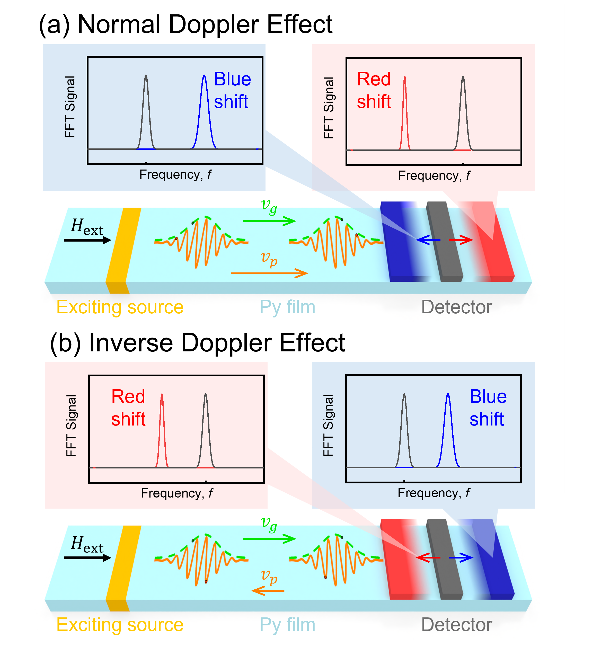
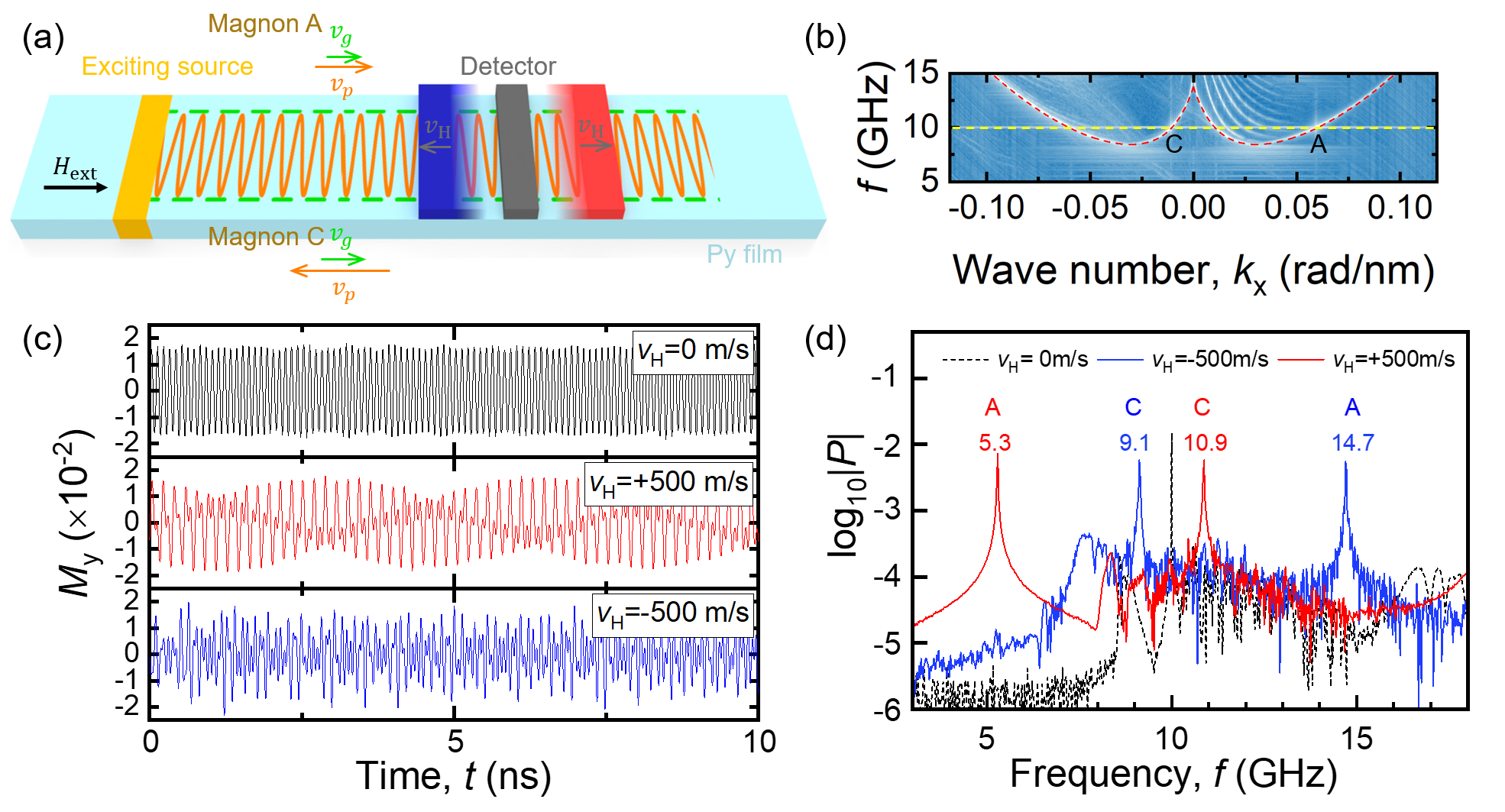
Here we introduce the spin wave Doppler effect, which could effectively control and detect the characteristics of spin waves.vlaminck2008current ; chauleau2014self ; xia2016doppler ; sugimoto2016observation ; kim2021current ; nakane2021current ; 2021Yu ; hu2024voltage In a spin wave system, the frequency of the spin wave will change when the source of the wave and the detector are in relative motion. By adjusting the relative motion speed between the source of the wave and the detector, the frequency of the spin wave can be changed, thereby achieving the detection of the spin wave. Additionally, the blue shift or red shift of spin waves is related to their group velocity and phase velocity. As illustrated in Fig.1(a), when the group velocity and phase velocity of the spin waves are parallel, and the detector approaches the spin wave source, the spin wave will exhibit a blue shift. Conversely, if the detector moves away from the spin wave source, the spin wave will exhibit a red shift. This is the well-known normal Doppler effect. However, if the group velocity and the phase velocity are anti-parallel, when the detector approaches the spin wave excitation source, the spin wave spectrum will show a red shift. When the detector moves away from the excitation source, the spin wave will show a blue shift. This unusual phenomenon of spin wave Doppler frequency shift is called the inverse spin wave Doppler effectstancil2006observation as shown in Fig.1(b). For BVMSW, spin waves at low wave numbers are expected to exhibit an inverse Doppler effect due to having anti-parallel phase and group velocitiesseddon2003observation ; stancil2006observation ; chumak2010reverse ; wessels2016direct . This inverse Doppler shift will help us better distinguishing SWs with different wave vectors.
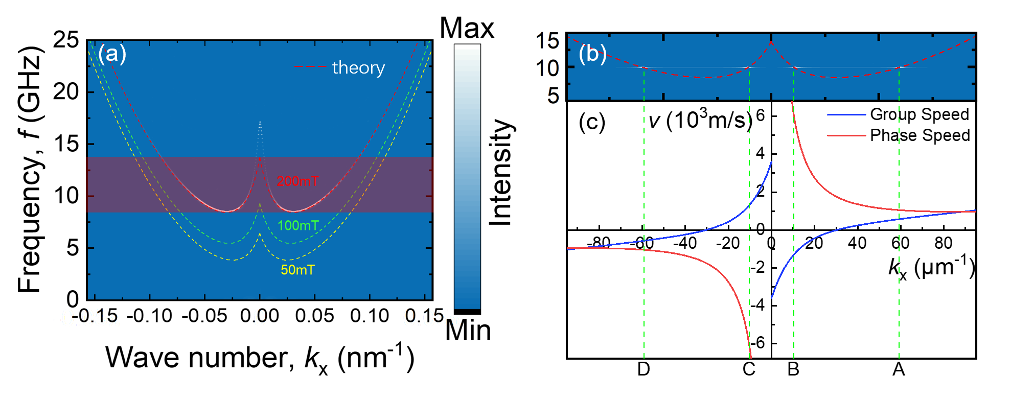
To confirm our hypothesis, we perform micromagnetic simulations by MuMax3vansteenkiste2014design to study the spin wave Doppler effect of BVMSWs in Permalloy film. We study a Permalloy film discretized using finite difference cells. The periodic boundary condition is used along y axis to avoid the boundary effect. The simulation parameters used are as follows: saturation magnetization , exchange constant , Gilbert damping .hu2022significant ; Cui2024Magnetic To prevent SW reflection at both ends, is increased following a squared pattern from 0.0001 to 0.1 at both end regions of the Py film ( nm < x < nm, nm < x < nm). An external magnetic field is applied to magnetize the Py film along +x axis. Two dimensional Fourier transform on in response to a sinc-based excitation field with , cutoff frequency and ns, at the center section () of Py film is performedKumar2012numerical . At first, the dispersion relations are obtained as shown in Fig.2(a). The dashed lines represent the theoretical calculations from the dispersion relation equations of BVMSWs in isotropic regions given as followkalinikos1986theory ; wang2022dual ; hu2024voltage :
where is the gyromagnetic ratio; is the permeability of free space; is the wave number; is the thickness of the magnetic film.
To enhance our understanding of the dispersion relation, we have plotted the calculated dispersion relations under external magnetic fields of and , as shown in Fig. 2(a). These calculations reveal that the negative dispersion relations are consistent from the magnetic resonant frequency () to the minimum cutoff frequency (), at which point the group velocity reaches zero. The cutoff frequency rises with increasing magnetic field strength. Although micro-magnetic simulations and theoretical calculations generally align across most wave numbers, discrepancies become significant at the smallest wave numbers. This mismatch arises from the challenges in simulating long-wavelength spin waves in Permalloy films, which are constrained by their finite size. Here, the simulation parameters of geometry were optimized to minimize deviations at the smallest wave numbers. Interestingly, a single frequency corresponds to two types of spin waves with distinct wave numbers in the range marked as red colour in Fig.2(a). To verify the unique properties, we present the dispersion relation for spin waves excited solely by a single frequency of , as depicted in Fig.2(b). It is evident that there are four distinct types of magnon vectors.
One of the significant properties of magnons with different wave numbers is the group velocity of spin waves , the velocity with which the modulation or envelope of the wave propagates through spacebailleul2003propagating . Generally, both the group and phase velocities are the same sign with the wave number, aka Magnon A and D in Fig.2(c). However, the group and phase velocities are opposite signs for the magnons B and C. This unique feature mainly comes from the negative group velocity of BVMSWs, where the sign of group velocity is opposite to the wave vector, their propagation directionstancil2006observation .
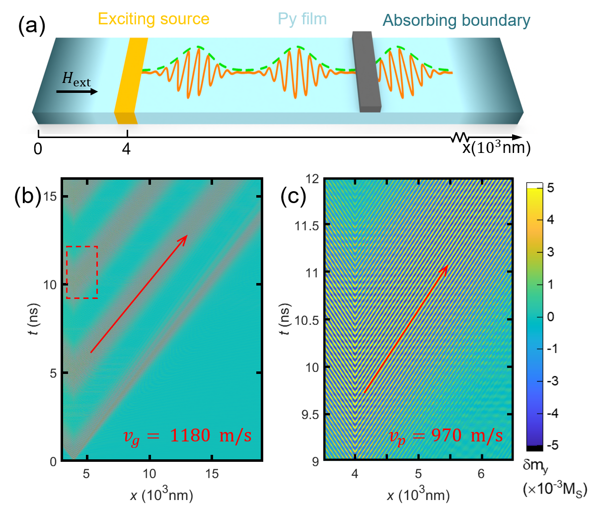
To further study the group and phase velocity properties of spin waves, we set a full-sized Py film as shown in Fig.3(a). Additionally, for concentration on SWs propagating along +x axis, we move the excitation field along -x axis to much closer to the absorbing boundary. Firstly, only one type of SWs is excited in wavepacks using single-frequency excitation , where , and , the modulation frequency . The image plots of simulated magnetization () as a function of time and space, as shown in Fig.3(b,c). The group velocity is estimated at , as observed from the modulated signal propagating through space in Fig. 3(b). The phase velocity is estimated at , based on the propagating carrier wave in Fig. 3(c), originating from the amplification region depicted in Fig. 3(b). These values are consistent with theoretical predictions, clearly confirming the distinguishable difference between the group and phase velocities of spin waves.
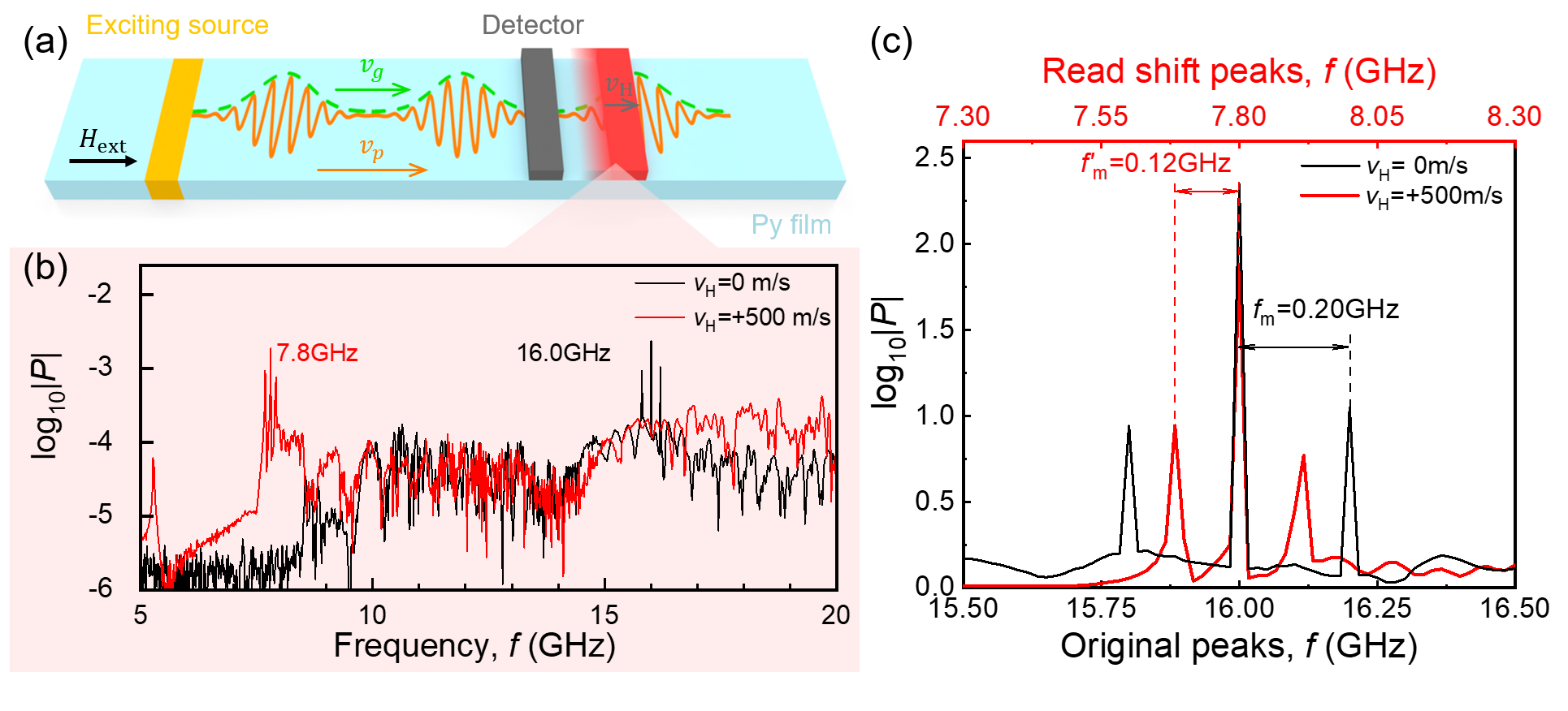
For analysis of the spin wave Doppler effect, we first fixed the detector (grey colour) by sampling from one discretization cell , as shown in Fig.4(a). Fast Fourier transform on the function is performed to obtain the spectrum of the unaltered signals of SW. And two secondary peaks are observed from the spectrum of the modulated spin waves in Fig.4(b). This unique spectrum could be understood by the form function of the modulated spin wave as . From Fig.4(c), we can clearly see that the gap between the main peak and the secondary peak is , identical to the frequency of modulated frequency of SW. Then, we implement detector moving along +x axis at velocity by continuous movement of sampling point on the Py film over one discretization cell during each time window in the simulationhu2024voltage . The spin wave spectrum is obtained for moving detector by performing an FFT on , as illustrated by the red curve in Fig.4(b). The main peak () is read as , a significant red shift of SW. The phase velocity could be evaluated as the value of based on the the normal Doppler frequency shift formula (See appendix). The change of gap between the main peak and the secondary peak is obtained as by the enlarged spectra with aligned main peaks in Fig.4(c). Actually, the frequency shift of the secondary peak gap can be used to estimate the group velocity of spin waves. The obtained group velocity from the formula (See appendix) with the value of is nearly consistent with the value obtained in Fig.3. This error arises from the fact that the frequency resolution of the FFT spectrum is only 0.01 GHz, and the frequency gap cannot be regarded as an infinitesimal quantity as shown in Fig.4(d). The result indicates that the group velocity-induced spin wave Doppler effect could be precisely analysed using the frequency shift difference of the main and secondary peaks, while also presents a straightforward method for approximating the group velocity of SWs.
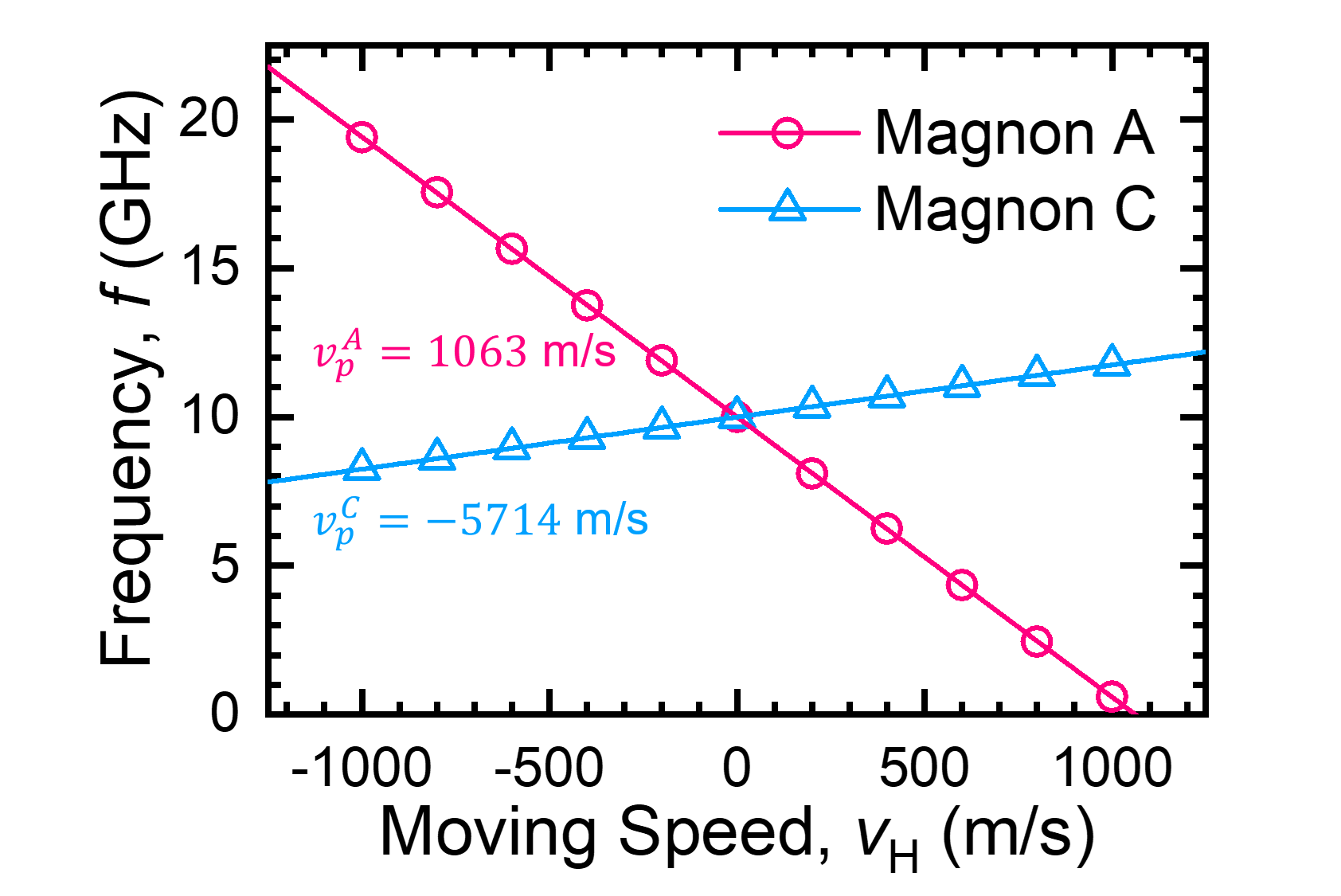
A single-frequency excitation source, defined by where and , was utilized in subsequent simulations. This frequency excites two types of SWs, as depicted by the dispersion relation of backward-volume magnetostatic spin waves in Fig.2(a). The dispersion relation of BVMSW shows two highlighted spots, which correspond to the magnon models A and C in Fig.5(b). In contrast, magnon modes B and D are suppressed due to spatial limitations along the negative x-axis. The design of the geometry thus plays a crucial role in accurately analyzing the spin wave Doppler effect. Initially, the time-dependent magnetization spectra were recorded by the detector under various motion scenarios, as illustrated in Fig.5(c). For a stationary detector (), the curve exhibits a standard sine function pattern, aligning with the spin wave’s excitation function. The frequency spectrum for this case shows a single peak at 10 GHz (black curve in Fig.5(d). Conversely, with the detector moving at , the curve resembles a modulated wave, as shown in Fig.5(c). This motion results in two distinct frequency peaks at 5.3 GHz and 10.9 GHz, depicted by the red curve in Fig.5(d). The red-shifted frequency peak at can be attributed to the normal Doppler effect, where the detector is positioned far from the source, primarily influenced by magnon A. Conversely, magnon C, moving in a scenario where phase and group velocities are anti-parallel, contributes to a blue-shifted frequency peak at , indicative of the inverse Doppler effect. Reversing the detector’s movement along the -x axis to a velocity of also distinctly produces two peaks in the frequency spectrum (blue curve in Fig.5(d)). A prominent blue-shifted peak at due to the normal Doppler effect from magnon A, and a smaller red-shifted peak from magnon C, consistent with the inverse Doppler effect. To accurately determine the phase velocities of magnons A and C, we simulated the frequency shifts across various detector velocities as displayed in Fig.6. By employing linear fitting, we calculated the phase velocities of magnon A and C are and , respectively. The results align well with those predicted from the dispersion relation in Fig.2. The negative phase velocity value for magnon C confirms the inverse Doppler effect. These observations offer a robust method for differentiating between the two magnon models through their Doppler shifts.
In summary, our study has revealed, in the case of BVMSWs, spin waves at low wave numbers display an inverse Doppler effect because their phase and group velocities are anti-parallel. Conversely, at high wave numbers, a normal Doppler effect occurs due to the parallel alignment of phase and group velocities. Analyzing the spin wave Doppler effect offers a novel perspective for understanding intrinsic interactions and can also help mitigate serious interference issues in the design of spin logic circuits.
Acknowledgements.
Appendix A Spin wave Doppler effect of phase and group velocity
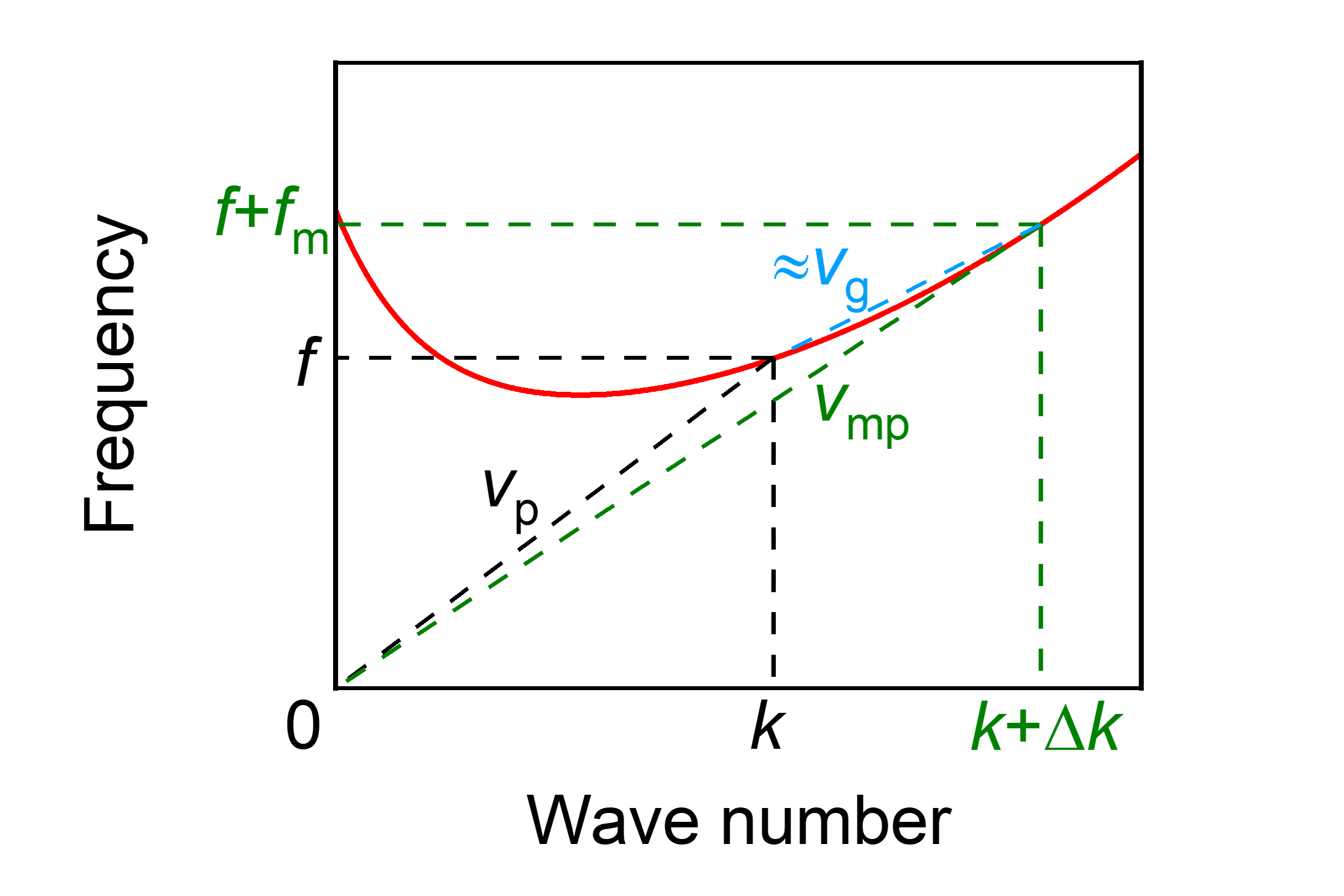
The definition of phase and group velocity:
| where represents the unit wavevector, as the same direction as both the phase velocity and the group velocity of the SW. | ||||
| When and are at relatively small values, the following approximation holds. | ||||
| Treat the original secondary peak as an independent SW. The frequency shift follows the Doppler formula, same as the main peak SW. | ||||
| where the secondary SW has a different phase velocity : | ||||
| The gap shift can be calculated by the difference of and : | ||||
References
- [1] Felix Bloch. Zur Theorie des Austauschproblems und der Remanenzerscheinung der Ferromagnetika, pages 295–335. Springer Berlin Heidelberg, Berlin, Heidelberg, 1932.
- [2] T. Holstein and H. Primakoff. Field dependence of the intrinsic domain magnetization of a ferromagnet. Phys. Rev., 58:1098–1113, Dec 1940.
- [3] Freeman J. Dyson. General theory of spin-wave interactions. Phys. Rev., 102:1217–1230, Jun 1956.
- [4] Eric Vogel. Technology and metrology of new electronic materials and devices. Nature nanotechnology, 2(1):25–32, 2007.
- [5] Sebastian Neusser and Dirk Grundler. Magnonics: Spin waves on the nanoscale. Advanced materials, 21(28):2927–2932, 2009.
- [6] Alexander Khitun, Mingqiang Bao, and Kang L Wang. Magnonic logic circuits. Journal of Physics D: Applied Physics, 43(26):264005, 2010.
- [7] Benjamin Lenk, Henning Ulrichs, Fabian Garbs, and Markus Münzenberg. The building blocks of magnonics. Physics Reports, 507(4-5):107–136, 2011.
- [8] Andrii V Chumak, Vitaliy I Vasyuchka, Alexander A Serga, and Burkard Hillebrands. Magnon spintronics. Nature physics, 11(6):453–461, 2015.
- [9] Thomas N Theis and H-S Philip Wong. The end of moore’s law: A new beginning for information technology. Computing in science & engineering, 19(2):41–50, 2017.
- [10] Philipp Pirro, Vitaliy I. Vasyuchka, Alexander A. Serga, and Burkard Hillebrands. Advances in coherent magnonics. Nature Reviews Materials, 6:1114 – 1135, 2021.
- [11] Benedetta Flebus, Dirk Grundler, Bivas Rana, Yoshichika Otani, Igor Barsukov, Anjan Barman, Gianluca Gubbiotti, Pedro Landeros, Johan Akerman, Ursula S Ebels, Philipp Pirro, V E Demidov, Katrin Schultheiss, Gyorgy Csaba, Qi Wang, Dmitri E. Nikonov, Florin Ciubotaru, Ping Che, Riccardo hertel, Teruo Ono, Dmytro Afanasiev, Johan H Mentink, Theo Rasing, Burkard Hillebrands, Silvia Viola Kusminskiy, Wei Zhang, Chunhui Rita Du, Aurore Finco, Toeno van der Sar, Yunqiu Kelly Luo, Yoichi Shiota, Joseph Sklenar, Tao Yu, and Jinwei Rao. The 2024 magnonics roadmap. Journal of Physics: Condensed Matter, 2024.
- [12] Richard W Damon and JR Eshbach. Magnetostatic modes of a ferromagnet slab. Journal of Physics and Chemistry of Solids, 19(3-4):308–320, 1961.
- [13] A. V. Sadovnikov, C. S. Davies, V. V. Kruglyak, D. V. Romanenko, S. V. Grishin, E. N. Beginin, Y. P. Sharaevskii, and S. A. Nikitov. Spin wave propagation in a uniformly biased curved magnonic waveguide. Phys. Rev. B, 96:060401, Aug 2017.
- [14] Kenji Kasahara, Ryusei Akamatsu, and Takashi Manago. Ferromagnetic-waveguide width dependence of propagation properties for magnetostatic surface spin waves. AIP Advances, 11(4):045308, 04 2021.
- [15] UK Bhaskar, Giacomo Talmelli, Florin Ciubotaru, Christoph Adelmann, and Thibaut Devolder. Backward volume vs damon–eshbach: A traveling spin wave spectroscopy comparison. Journal of Applied Physics, 127(3), 2020.
- [16] Vincent Vlaminck and Matthieu Bailleul. Current-induced spin-wave doppler shift. Science, 322(5900):410–413, 2008.
- [17] J-Y Chauleau, HG Bauer, HS Körner, J Stigloher, M Härtinger, G Woltersdorf, and CH Back. Self-consistent determination of the key spin-transfer torque parameters from spin-wave doppler experiments. Physical Review B, 89(2):020403, 2014.
- [18] Hong Xia, Jie Chen, Xiaoyan Zeng, and Ming Yan. Doppler effect in a solid medium: Spin wave emission by a precessing domain wall drifting in spin current. Physical Review B, 93(14):140410, 2016.
- [19] Satoshi Sugimoto, Mark C Rosamond, Edmund H Linfield, and Christopher H Marrows. Observation of spin-wave doppler shift in micro-strips for evaluating spin polarization. Applied Physics Letters, 109(11), 2016.
- [20] Dong-Hyun Kim, Se-Hyeok Oh, Dong-Kyu Lee, Se Kwon Kim, and Kyung-Jin Lee. Current-induced spin-wave doppler shift and attenuation in compensated ferrimagnets. Physical Review B, 103(1):014433, 2021.
- [21] Jotaro J Nakane and Hiroshi Kohno. Current-induced spin-wave doppler shift in antiferromagnets. Journal of the Physical Society of Japan, 90(10):103705, 2021.
- [22] Tao Yu, Chen Wang, Michael A. Sentef, and Gerrit E. W. Bauer. Spin-Wave Doppler Shift by Magnon Drag in Magnetic Insulators. Phys. Rev. Lett., 126:137202, 2021.
- [23] Shaojie Hu, Kang Wang, Tai Min, and Takashi Kimura. Voltage-controlled spin-wave doppler shift in a ferromagnetic/ferroelectric heterojunction. Physical Review Applied, 22(1):014085, 2024.
- [24] Daniel D Stancil, Benjamin E Henty, Ahmet G Cepni, and JP Van’t Hof. Observation of an inverse doppler shift from left-handed dipolar spin waves. Physical Review B—Condensed Matter and Materials Physics, 74(6):060404, 2006.
- [25] N Seddon and T Bearpark. Observation of the inverse doppler effect. Science, 302(5650):1537–1540, 2003.
- [26] AV Chumak, P Dhagat, A Jander, AA Serga, and B Hillebrands. Reverse doppler effect of magnons with negative group velocity scattered from a moving bragg grating. Physical Review B—Condensed Matter and Materials Physics, 81(14):140404, 2010.
- [27] Philipp Wessels, Andreas Vogel, Jan-Niklas Tödt, Marek Wieland, Guido Meier, and Markus Drescher. Direct observation of isolated damon-eshbach and backward volume spin-wave packets in ferromagnetic microstripes. Scientific reports, 6(1):22117, 2016.
- [28] Arne Vansteenkiste, Jonathan Leliaert, Mykola Dvornik, Mathias Helsen, Felipe Garcia-Sanchez, and Bartel Van Waeyenberge. The design and verification of mumax3. AIP advances, 4(10), 2014.
- [29] Shaojie Hu, Xiaomin Cui, Kang Wang, Satoshi Yakata, and Takashi Kimura. Significant modulation of vortex resonance spectra in a square-shape ferromagnetic dot. Nanomaterials, 12(13), 2022.
- [30] Xiaomin Cui, Shaojie Hu, Yohei Hidaka, Satoshi Yakata, and Takashi Kimura. Magnetic vortex polarity reversal induced gyrotropic motion spectrum splitting in a ferromagnetic disk. Journal of Physics D: Applied Physics, 57(39):395002, jul 2024.
- [31] Dheeraj Kumar, Oleksandr Dmytriiev, Sabareesan Ponraj, and Anjan Barman. Numerical calculation of spin wave dispersions in magnetic nanostructures. Journal of Physics D: Applied Physics, 45(1):015001, dec 2011.
- [32] BA Kalinikos and AN Slavin. Theory of dipole-exchange spin wave spectrum for ferromagnetic films with mixed exchange boundary conditions. Journal of Physics C: Solid State Physics, 19(35):7013, 1986.
- [33] Kang Wang, Shaojie Hu, Fupeng Gao, Miaoxin Wang, and Dawei Wang. Dual function spin-wave logic gates based on electric field control magnetic anisotropy boundary. Applied Physics Letters, 120(14), 2022.
- [34] Matthieu Bailleul, Dominik Olligs, and Claude Fermon. Propagating spin wave spectroscopy in a permalloy film: A quantitative analysis. Applied Physics Letters, 83(5):972–974, 2003.