Notes on translating solitons for Mean Curvature Flow

Mean curvature flow is an exciting area of mathematical research. It is situated at the crossroads of several scientific disciplines: geometric analysis, geometric measure theory, partial differential equations, differential topology, mathematical physics, image processing, computer-aided design, among others. In these notes, we give a brief introduction to mean curvature flow and we describe recent progress on translators, an important class of solutions to mean curvature flow.

In physics, diffusion is a process which equilibrates spatial variations in concentration. If we consider a initial concentration $u_{0}$ on a domain $\Omega\subseteq\mathbf{R}^{2}$ and seek solutions of the linear heat equation $\frac{\partial}{\partial t}u-\operatorname{\Delta}u=0,$ with initial data $u_{0}$ and natural boundary conditions on $\partial\Omega$, we obtain smoothed concentrations $\{u_{t}\}_{t>0}$.

If we are interested in the smoothing of perturbed surface geometries, it make sense to use analogous strategies. The geometrical counterpart of the Euclidean Laplace operator $\operatorname{\Delta}$ on a smooth surface $M^{2}\subset\mathbf{R}^{3}$ (or more generally, a hypersurface $M^{n}\subset\mathbf{R}^{n+1}$) is the Laplace-Beltrami operator, which we will denote as $\operatorname{\Delta}_{M}$. Thus, we obtain the geometric diffusion equation

for the coordinates x of the corresponding family of surfaces $\{M_{t}\}_{t\in[0,T)}.$

A classical formula (see [hildebrandt], for instance) says that, given a hypersurface in Euclidean space, one has:

where $\vec{H}$ represents the mean curvature vector. This means that (1.1) can be written as:

Using techniques of parabolic PDE’s it is possible to deduce the existence and uniqueness of the mean curvature flow for a small time period in the case of compact manifolds (for details see [regularityTheoryMCF], [LecturesNotesOnMCF], among others).

The mean curvature is known to be the first variation of the area functional $M\mapsto\int_{M}d\mu$ (see [colding-minicozzi, meeks-perez].) We will obtain for the $\operatorname{Area}(\Omega(t))$ of a relatively compact $\Omega(t)\subset M_{t}$ that

In other words, we get that the mean curvature flow is the corresponding gradient flow for the area functional:

Moreover, we also have a nice maximum principle for this particular diffusion equation.

Similarly, convexity and mean convexity are preserved:

• •

  If the initial hypersurface $M$ is convex (i.e., all the geodesic curvatures are positive, or equivalently $M$ bounds a convex region of $\mathbf{R}^{n+1}$), then $M_{t}$ is convex, for any $t$.

• •

  If $M$ is mean convex ($H>0$), then $M_{t}$ is also mean convex, for any $t$.

Moreover, mean curvature flow has a property which is similar to the eventual simplicity for the solutions of the heat equation. This result was proved by Huisken and asserts:

As a consequence of the above theorems we have.

A natural question is: What can we say when $M$ is not compact? In this case, we can have long-time existence. A trivial example is the case of a complete, properly embedded minimal hypersurface $M$ in $\mathbf{R}^{n+1}$. Under the mean curvature flow, $M$ remains stationary, so the flow exists for all time. If we are looking for non-stationary examples, then we can consider the following example:

Throughout this section, we consider a fixed compact initial hypersurface $M$. Consider the maximal time $T=T_{M}$ such that a smooth solution of the MCF $F:M\times[0,T)\to\mathbf{R}^{n+1}$ as in Theorem 1.1 exists. Then the embedding vector $F$ is uniformly bounded according to Theorem 1.3. It follows that some spatial derivatives of the embedding $F_{t}$ have to become unbounded as $t\nearrow T$. Otherwise, we could apply Arzelà-Ascoli Theorem and obtain a smooth limit hypersurface, $M_{T}$, such that $M_{t}$ converges smoothly to $M_{T}$ as $t\nearrow T$. This is impossible because, in such a case, we could apply Theorem 1.1 to restart the flow. In this way, we could extend the flow smoothly all the way up to $T+\varepsilon$, for some $\varepsilon>0$ small enough, contradicting the maximality of $T$. In fact, Huisken [huisken84, Theorem 8.1] showed that the second spatial derivative (i.e, the norm of the second fundamental form) blows up as $t\to T.$

We would like to say more about the “blowing-up” of the norm of $A$, as $t\nearrow T.$ The evolution equation for $|A|^{2}$ is

Define

Using Hamilton’s trick (see [LecturesNotesOnMCF]) we deduce that $|A|^{2}_{\max}$ is locally Lipschitz and that

where $p_{0}$ is any point where $|A|^{2}(\cdot,t_{0})$ reaches its maximum. Thus, using the above expression, we have

It is well known that the Hessian of $|A|$ is negative semi-definite at any maximum. In particular the Laplacian of $|A|$ at these points is non-positive. Hence,

Notice that $|A|_{\text{max}}^{2}$ is always positive, since otherwise at some instant $t$ we would have $|A(\cdot,t)|\equiv 0$ along $M_{t}$, which would imply that $M_{t}$ is totally geodesic and therefore a hyperplane in $\mathbf{R}^{n+1}$, contrary to the fact that the initial surface was compact.

So, one can prove that $1/|A|_{\text{max}}^{2}$ is locally Lipschitz. Then the previous inequality allows us to deduce that:

Integrating (respect to time) in any sub-interval $[t,s]\subset[0,T)$ we get

As $|A(\cdot,t)|$ is not bounded as to tends to $T$, there exists a time sequence $s_{i}\nearrow T$ such that

Substituting $s=s_{i}$ in the above inequality and taking the limit as $i\to\infty$, we get

We collect all this information in the next proposition.

So we have the following improved version of Theorem 1.1:

We conclude this brief section by pointing out that there have been substantial breakthroughs in the study and understanding of the singularities of Type I, whereas Type II singularities have been much more difficult to study. This seems reasonable since, according to the above definition and the results we have seen, the singularities of Type I are those for which one has the best possible control of blow-up of the second fundamental form.

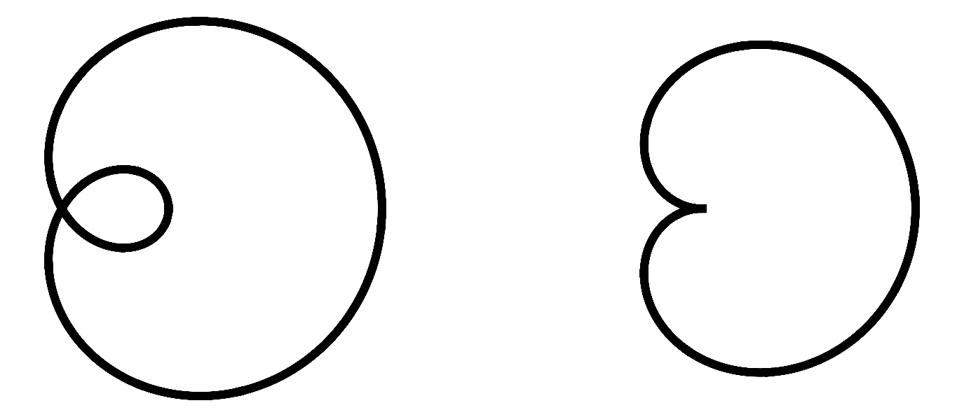
A standard example of Type II singularity is given by a loop pinching off to a cusp (see Figure 3). S. Angenent [An1] proved, in the case of convex planar curves, that singularities of this kind are asymptotic (after rescaling) to the above mentioned grim reaper curve (1.3), which moves set-wise by translation. In this case, up to inner diffeomorphisms of the curve, it can be seen as a solution of the curve shortening flow which evolves by translations and is defined for all time. In this paper we are interested in this type of solitons, which we will call translating solitons (or translators) from now on. Summarizing this information, we make the following definition:

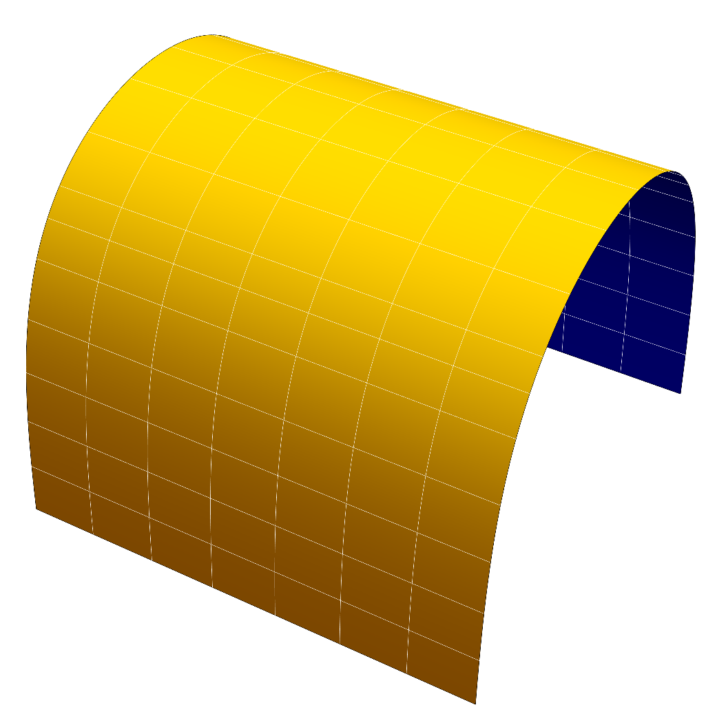
The cylinder over a grim-reaper curve, i.e. the hypersurface in $\mathbf{R}^{n+1}$ parametrized by $\mathscr{G}:\left(-\tfrac{\pi}{2},\tfrac{\pi}{2}\right)\times\mathbf{R}^{n-1}\longrightarrow\mathbf{R}^{n+1}$ given by

is a translating soliton. It appears as limit of sequences of parabolic rescaled solutions of mean curvature flows of immersed mean convex hypersurfaces. For example, we can take product of the loop pinching off to a cusp times $\mathbf{R}^{n-1}$. We can produce others examples of solitons just by scaling and rotating the grim reaper. In this way, we obtain a $1-$parameter family of translating solitons parametrized by $\mathscr{G}_{\theta}:\left(-\tfrac{\pi}{2\cos(\theta)},\tfrac{\pi}{2\cos(\theta)}\right)\times\mathbf{R}^{n-1}\longrightarrow\mathbf{R}^{n+1}$

where $\theta\in[0,\pi/2).$ Notice that the limit of the family $F_{\theta}$, as $\theta$ tends to $\pi/2$, is a hyperplane parallel to $\mathbf{e}_{n+1}$.

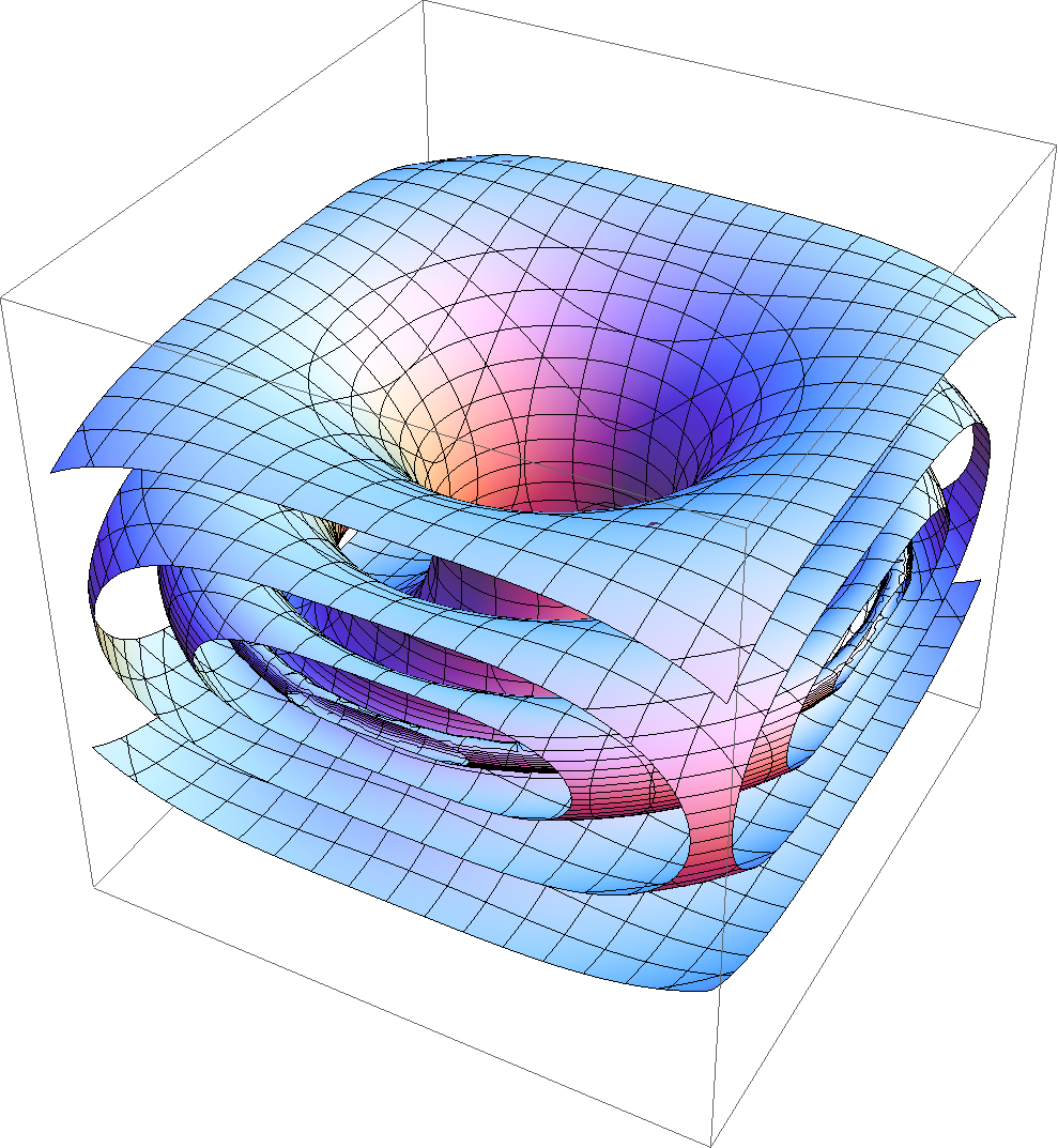
Besides the grim reapers that we have already described, the last decades have witnessed the appearance of numerous examples of translators. Clutterbuck, Schnürer and Schulze [CSS] (see also [Altschuler-Wu]) proved that there exists an entire graphical translator in $\mathbf{R}^{n+1}$ which is rotationally symmetric, strictly convex with translating velocity $-\mathbf{e}_{n+1}$. This example is known as the translating paraboloid or bowl soliton. Moreover, they classified all the translating solitons of revolution, giving a one-parameter family $\{W^{n}_{\lambda}\}_{\lambda>0}$ of rotationally invariant cylinders called translating catenoids. The parameter $\lambda$ controls the size of the neck of each translating soliton. The limit, as $\lambda\to 0$, of $W^{n}_{\lambda}$ consists of two superimposed copies of the bowl soliton with a singular point at the axis of symmetry. Furthermore, all these hypersurfaces have the following asymptotic expansion as r approaches infinity:

where $r$ is the distance function in $\mathbf{R}^{n}$.

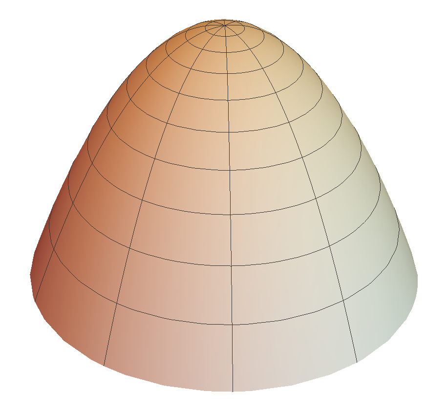
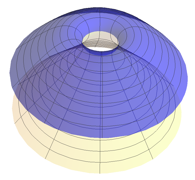
These rotationally symmetric translating catenoids can be seen as the desingularization of two paraboloids connected by a small neck of some radius.

Recall that the Costa-Hoffman-Meeks surfaces can be regarded as desingularizations of a plane and catenoid: a sequence of Costa-Hoffman-Meeks surfaces with genus tending to infinity converges (if suitably scaled) to the union of a catenoid and the plane through its waist. This suggests that one try to construct translators by desingularizing the union of a translating catenoid and a bowl solition. Dávila, del Pino, and Nguyen  [DDPN] were able to do that (for large genus) by glueing methods, replacing the circle of intersection by a surface similar to the singly periodic Scherk minimal surface (see also [smith].) Previously, Nguyen in [Nguyen09],[Nguyen13] and [Nguyen15] had used similar techniques to desingularize the intersection of a grim reaper and a plane. In this way she obtained a complete periodic embedded translator of infinite genus, that she called a translating trident.

Once this abundance of translating solitons is guaranteed, there arises the need to classify them. One of the first classification results was given by X.-J. Wang in [wang]. He characterized the bowl soliton as the only convex translating soliton which is an entire graph.

Very recently, J. Spruck and L. Xiao [spruck-xiao] have proved that a complete translating soliton which is graph over a domain in $\mathbf{R}^{2}$ must be convex (see Section 6 below.) So, combining both results we have:

Using the Alexandrov method of moving hyperplanes, Martín, Savas-Halilaj, and Smoczyk [mss] showed that the bowl soliton is the only translator (not assumed to be graphical) that has one end and is $C^{\infty}$-asymptotic to a bowl soliton. Hershkovits [Her18] improved this by showing uniqueness of the bowl soliton among (not necessarily graphical) translators that have one cylindrical end (and no other ends). Haslhofer [Has15] proved a related result in higher dimensions: he showed that any translator in $\mathbf{R}^{n+1}$ that is noncollapsed and uniformly $2$-convex must be the $n$-dimensional bowl soliton. At this point, we would like to mention the recent classification result of Brendle and Choi [brendle]. They prove that the rotationally symmetric bowl soliton is the only noncompact ancient solution of mean curvature flow in $\mathbf{R}^{3}$ which is strictly convex and noncollapsed.

Martín, Savas-Halilaj and Smoczyk also obtained one of the first characterizations of the family of tilted grim reapers:

If a translator $M$ is the graph of function $u:\Omega\subset\mathbf{R}^{n}\to\mathbf{R}$, we will say that $M$ is a translating graph; in that case, we also refer to the function $u$ as a translator, and we say that $u$ is complete if its graph is a complete submanifold of $\mathbf{R}^{n+1}$. Thus $u:\Omega\subset\mathbf{R}^{n}\to\mathbf{R}$ is a translator if and only if it solves the translator equation (the nonparametric form of (3.1)):

The equation can also be written as

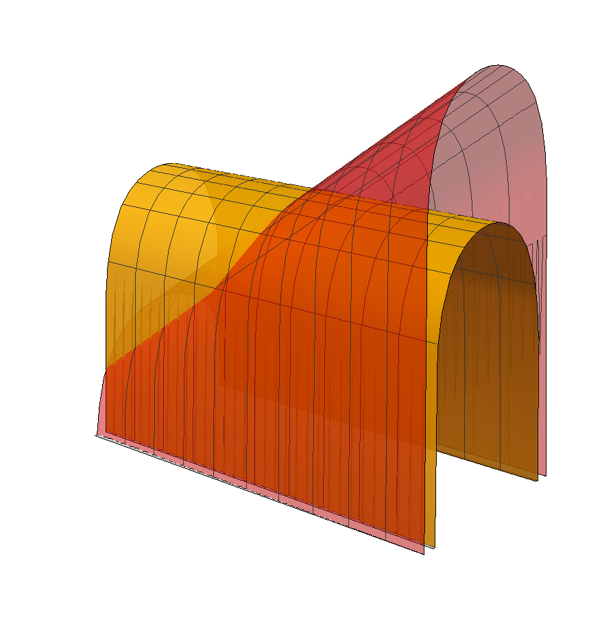
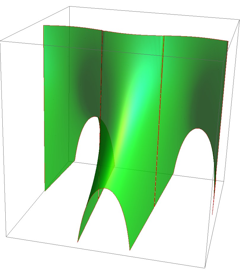
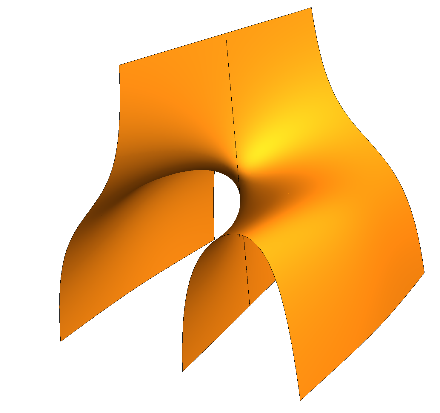
In a recent preprint, we classify all complete translating graphs in $\mathbf{R}^{3}$. In two other papers [families-1, families-2], we construct new families of complete, properly embedded (non-graphical) translators: a two-parameter family of translating annuli, examples that resemble Scherk’s minimal surfaces, and examples that resemble helicoids. In [families-2], we also construct several new families of complete translators that are obtained as limits of the Scherk-type translators mentioned above. They include a $1$-parameter family of single periodic surfaces called Scherkenoids (see Fig. 6) and a simply-connected translator called the pitchfork translator (see Fig. 7). The pitchfork translator resembles Nguyen’s translating tridents [Nguyen09] (see also [families-1.5]): like the tridents, it is asymptotic to a plane as $z\to\infty$ and to three parallel planes as $z\to-\infty$. However, the pitchfork has genus $0$, whereas the tridents have infinite genus.

As a consequence of Theorem 4.2, we have that every translator $\mathbf{R}^{3}$ with zero Gauss curvature is a grim reaper surface, a tilted grim reaper surface, or a vertical plane.

In addition to the examples described in the previous section, Ilmanen (in unpublished work) proved that for each $0<k<1/2$, there is a translator $u:\Omega\to\mathbf{R}$ with the following properties: $u(x,y)\equiv u(-x,y)\equiv u(x,-y)$, $u$ attains its maximum at $(0,0)\in\Omega$, and

The domain $\Omega$ is either a strip $\mathbf{R}\times(-b,b)$ or $\mathbf{R}^{2}$. He referred to these examples as $\operatorname{\Delta}$-wings. As $k\to 0$, he showed that the examples converge to the grim reaper surface. Uniqueness (for a given $k$) was not known. It was also not known which strips $\mathbf{R}\times(-b,b)$ occur as domains of such examples. The main result in [himw] is the following:

Although the paper [himw] is primarily about translators in $\mathbf{R}^{3}$, the last sections extend Ilmanen’s original proof to get $\operatorname{\Delta}$-wings in $\mathbf{R}^{n+1}$ that have prescribed principal curvatures at the origin. For $n\geq 3$, the examples include entire graphs that are not rotationally invariant. At the end of the paper, we modify the construction to produce a family of $\operatorname{\Delta}$-wings in $\mathbf{R}^{n+2}$ over any given slab of width $>\pi$. See [wang] for a different construction of some higher dimensional graphical translators.

One of the fundamental results in the recent development of soliton theory has been the paper by Spruck and Xiao [spruck-xiao], where they proved that complete graphical translators (or, more generally, complete translators of positive mean curvature) are convex. The ideas contained in this paper are really inspiring and we would like to provide a slightly simplified exposition of their proof.

At any non-umbilic point, we let $\kappa_{1}>\kappa_{2}$ be the principal curvatures and $H=\kappa_{1}+\kappa_{2}>0$ be the mean curvature. We let $v_{1}$ and $v_{2}$ be the principal direction unit vector fields, so

Note $\nabla_{u}v_{1}$ is perpendicular to $v_{1}$. Thus

for some functions $\alpha_{1}$ and $\alpha_{2}$. Since $0=\nabla_{v_{i}}(v_{1}\cdot v_{2})=(\nabla_{v_{i}}v_{1})\cdot v_{2}+v_{1}\cdot(\nabla_{v_{i}}v_{2})$, we see that

Thus

But $\nabla_{u}v_{1}$ is perpendicular to $v_{1}$, so $A(\nabla_{u}v_{1},v_{1})\equiv 0$. Thus

In particular,

where $h_{ij}=A(v_{i},v_{j})$ and $h_{ij,k}=(\nabla_{v_{k}}A)(v_{i},v_{j})$. From $A(v_{1},v_{2})\equiv 0$, we see that

by (6.1) and (6.2). Thus

Also, if we let $u_{i}=v_{i}$ at a particular point and extend by parallel transport on radial geodesics, we have

Thus

where

(The second equality follows from the Codazzi equations.)

Now suppose the surface is a translator. Then, we have that (see [spruck-xiao, Lemma 2.1] or [mss, Lemma 2.1]):

Hence,

by (6.3). Thus

Recall that the drift Laplacian (see (3.7)) is given by

Likewise,

Adding these gives

From (6.7) and (6.8),

Thus

so