University of Manchester, M13 9PL, U.K. 33institutetext: Jagiellonian University, ul. prof. Stanislawa Łojasiewicza 11, 30-348 Kraków, Poland
e1e-mail: Petr.Baron@ifj.edu.pl \thankstexte2e-mail: Michael.Seymour@manchester.ac.uk \thankstexte3e-mail: Andrzej.Siodmok@uj.edu.pl
Novel approach to measure quark/gluon jets at the LHC
Abstract
In this paper, we present a new proposal on how to measure quark/gluon jet properties at the LHC. The measurement strategy takes advantage of the fact that the LHC has collected data at different energies. Measurements at two or more energies can be combined to yield distributions of any jet property separated into quark and gluon jet samples on a statistical basis, without the need for an independent event-by-event tag. We illustrate our method with a variety of different angularity observables, and discuss how to narrow down the search for the most useful observables.
1 Introduction
Experimentally, we can study partons (quarks and gluons) by analyzing jets (narrow, energetic sprays of particles) whose kinematic characteristics mirror those of an initiating parton that cannot be directly measured. By employing an appropriate jet definition, it becomes possible to establish a link between jet measurements obtained from clusters of hadrons and calculations performed on clusters of partons. In a more ambitious approach, it is conceivable to attempt jet tagging with a well-defined flavour label, thereby increasing the proportion of, for instance, gluon-tagged jets compared to quark-tagged jets. The capacity to differentiate quark jets from gluon jets on an event-by-event basis has the potential to considerably increase the scope and sensitivity of numerous new-physics studies at the Large Hadron Collider (LHC) Gallicchio:2011xq ; FerreiradeLima:2016gcz ; Whitmore:2019cri ; Bhattacherjee:2016bpy ; Li:2023tcr ; Wong:2023vpx . This is because Beyond the Standard Model signals are often dominated by quarks while the corresponding Standard Model backgrounds are dominated by gluons Gallicchio:2012ez ; Sakaki:2018opq .
As well as proposing an observable that can distinguish quark jets and gluon jets Fodor:1989ir ; Pumplin:1991kc ; Stewart:2022ari ; Metodiev:2018ftz ; Frye:2017yrw ; Davighi:2017hok ; Goncalves:2015prv ; Dreyer:2021hhr ; Bright-Thonney:2018mxq ; Bhattacherjee:2015psa ; Komiske:2018vkc ; Komiske:2022vxg , any quantitative analysis must also propose how to calibrate that observable by independently tagging quark and gluon jet samples. In some studies, this has been done by calibrating against Monte Carlo samples in which the “truth” flavour of the jet is known. However, one might worry about whether event generators make sufficiently reliable predictions of these flavour-dependent properties Gras:2017jty ; Reichelt:2017hts ; Siodmok:2017oyv and, indeed, this is something one would like to test against the data. In other studies, another method is used to tag the jet flavour, for example the hard process dependence ATLAS:2014vax ; Aggleton:2021fcw , and used to calibrate the measurement of the proposed observable. Here, one would worry that the two tagging methods are correlated, yielding a biased measurement of the jet property.
In this paper, we study a variety of angularity observables as measures of quark/gluon jet differences. The main new ingredient we propose is the calibration of those differences using the dependence on the centre-of mass energy of the Large Hadron Collider. The idea is that the properties of jets of a given flavour and transverse momentum, if suitably defined, are almost entirely independent of the jet’s production mechanism, i.e. its rapidity, the energy of the collision, the colliding beam types, parton distributions, etcSeymour:1994by , but the fraction of jets of a given flavour at fixed transverse momentum does depend on all those factors, in particular the collision energy. However, those jet fractions can be reliably predicted. Thus, the energy-dependence can be used to extract the flavour-dependent properties on a statistical basis.
This paper is organised as follows: in Section 2, we present the measurement strategy; then, in Section 3, we discuss important systematic effects; in Section 4, we present measures that determine the quality of observables; in Section 5 we provide the main results, and finally in Section 6 we summarise the study.
2 Measurement strategy
The LHC has collected data at many different energies: GeV, TeV, TeV, TeV, TeV and TeV and will also take data at TeV. There is great potential to significantly increase the research potential of LHC by constructing new experimental strategies that exploit this unique situation. A measurement strategy based on the flexibility of the LHC to run at variable beam energies has already been successfully studied in the case of measuring the mass of the boson Krasny:2007cy ; Krasny:2010vd and the difference in the mass of the and bosons Fayette:2009yvt . In these publications, this flexibility was shown to be helpful in defining observables that are insensitive to ambiguities in the modelling, as well as in minimising the impact of systematic errors in the -boson mass measurement. This was achieved through the construction of observables that included the ratio of physical quantities measured at different energies. A second example of this type of measurement that we are aware of is Mangano:2012mh , in which the authors used both the ratios of cross sections, and the ratios of cross-sectional ratios between different centre-of-mass energies at the LHC to study the possibilities for precise measurements and BSM sensitivity. Sadly, despite many advantages, the idea of using LHC data collected at different energies to construct new robust observables was not exploited almost at all at LHC. The aim of this study is to change the situation and use this unique opportunity to construct new observables that are sensitive to the differences between quark and gluon jets.
The Tevatron collider also ran at different energies: GeV and TeV. The Tevatron experiments, CDF and D0, exploited this to some extent for parton distribution function measurements, but to our knowledge, only one analysis of final-state jet properties that combined measurements at the two energies was publishedD0:2001ab ; D0:2001nam . This followed essentially the same method we will apply to LHC events below, to extract the distribution of subjets within quark and gluon jets.
In leading-order QCD, the fraction of final-state jets that are of gluon origin increases with decreasing
| (1) |
where is the transverse momentum of a jet, is the proton-proton collision energy, and is the momentum fraction of the initial-state partons within the proton. This is mainly due to the dependence of the parton distribution function (PDF). For fixed , the gluon jet fraction therefore increases when is increased. This suggests an experimentally accessible way to define jet samples with different mixtures of quarks and gluons by varying . The main advantage of this approach is that the construction of an observable at different energies allows a single set of experimental cuts to be used to select jets, keeping all detector parameters unchanged, and, in this way, reducing many systematic errors. Let us provide one example of how the measurement can be biased when we use different selection criteria for quark and gluon samplesOPAL:1991ssr ; ATLAS:2014vax ; CMS:2021iwu . Based on the colour factor we could naively expect the “quark” jets to be much narrower than the “gluon” jets. However, the Monte Carlo simulations show that a high quark jet is narrower than a low jet, biasing the entire measurement if we define quark- and gluon-enriched samples using different ranges. At a more subtle level, even for jets at a given value of and rapidity, it might be thought that a cut on the rapidity of the recoiling jet in the dijet pair could be used to vary the quark to gluon mix (the so-called “same-side opposite-side” method). However, as shown in Forshaw:1999iv , colour-coherence effects in the hard process mean that the properties of a quark or gluon jet of fixed kinematics (specifically, the amount of soft radiation into it) respond to the rapidity of the other jet and only in an inclusive sample are the jet properties of a given flavour independent of the collider energy, type, etc. The strategy we present here, by construction, will be almost free from such bias.
There are many ways to define quark and gluon-jet discrimination observables Fodor:1989ir ; Pumplin:1991kc ; Stewart:2022ari ; Metodiev:2018ftz ; Frye:2017yrw ; Davighi:2017hok ; Goncalves:2015prv ; Dreyer:2021hhr ; Bright-Thonney:2018mxq ; Bhattacherjee:2015psa ; however, we follow Gras:2017jty and use five generalised angularities Larkoski:2014pca :
Here, multiplicity is the hadron multiplicity within the jet, was defined in Pandolfi:1480598 ; Chatrchyan:2012sn 111 In Pandolfi:1480598 ; Chatrchyan:2012sn , . Therefore, what we call in our work is actually its square (in the same way that what we call mass is actually proportional to the mass-squared of the jet)., LHA refers to the “Les Houches Angularity” (named after the workshop venue where this study was initiated Badger:2016bpw ), width is closely related to jet broadening Catani:1992jc ; Rakow:1981qn ; Ellis:1986ig , and mass is closely related to jet thrust Farhi:1977sg . In general an angularity is defined as where runs over the constituents of the jet particles, is a transverse momentum fraction, here is the rapidity-azimuth distance to the jet axis and is the jet-radius parameter.
Let denote an angularity in a jet from a mixed sample of quark and gluon jets and denote the value of one bin of a normalised histogram of . i.e. is the value of averaged over the th bin, where is the number of jets. We can express as a linear combination of the angularity distribution in a gluon and quark jet:
| (2) |
The coefficients are the fractions of gluon and quark () jets in the mixed sample. Let us consider that we measure just two similar samples of jets at two different energies and and we assume that and are independent of (we will return to this assumption later). We then obtain:
| (3) |
and
| (4) |
where and are experimental measurements in mixed jet samples at and , and and are fractions of gluon jets in the two samples. The jet fraction is provided by Monte Carlo simulation.
2.1 Event Selection
To prepare the most efficient measurement strategy, we study the production of dijets at the LHC at different energies: GeV, TeV, TeV and TeV. The samples were generated using two different Monte Carlo generators: Herwig 7.2.2 Bellm:2015jjp ; Bellm:2019zci with its default settings with PDF set MMHT2014lo68cl Harland-Lang:2014zoa , Pythia 8.240 Sjostrand:2014zea ; Bierlich:2022pfr using its default settings with PDF set NNPDF2.3 QCD+QED LO Ball:2013hta and the jets were reconstructed using the Anti- algorithm Cacciari:2008gp implemented in the FastJet package Cacciari:2005hq ; Cacciari:2011ma . We require exactly two jets that satisfy the following criteria:
| (5) |
and
| (6) |
where is the transverse momentum of the leading jet and is the transverse momentum of the subleading jet. We investigated five different jet radii , , , , , four different transverse momentum cuts , , and GeV. In addition to directly measuring the angularities, we also want to test the impact of jet grooming (see e.g. Butterworth:2008iy ; Ellis:2009su ; Ellis:2009me ; Krohn:2009th ). As one grooming example, we use the modified mass drop tagger (MMDT) with Butterworth:2008iy ; Dasgupta:2013ihk (equivalently, soft drop declustering with Larkoski:2014wba ) and .
2.2 Example of deriving q/g multiplicity (, GeV) using 900–13000 GeV
To determine the multiplicity of charged particles in gluon and quark jets we perform the following steps:
Step 1: Derive gluon fraction – parton level simulation (i.e. without hadronization and parton shower)
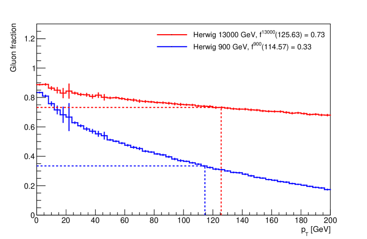
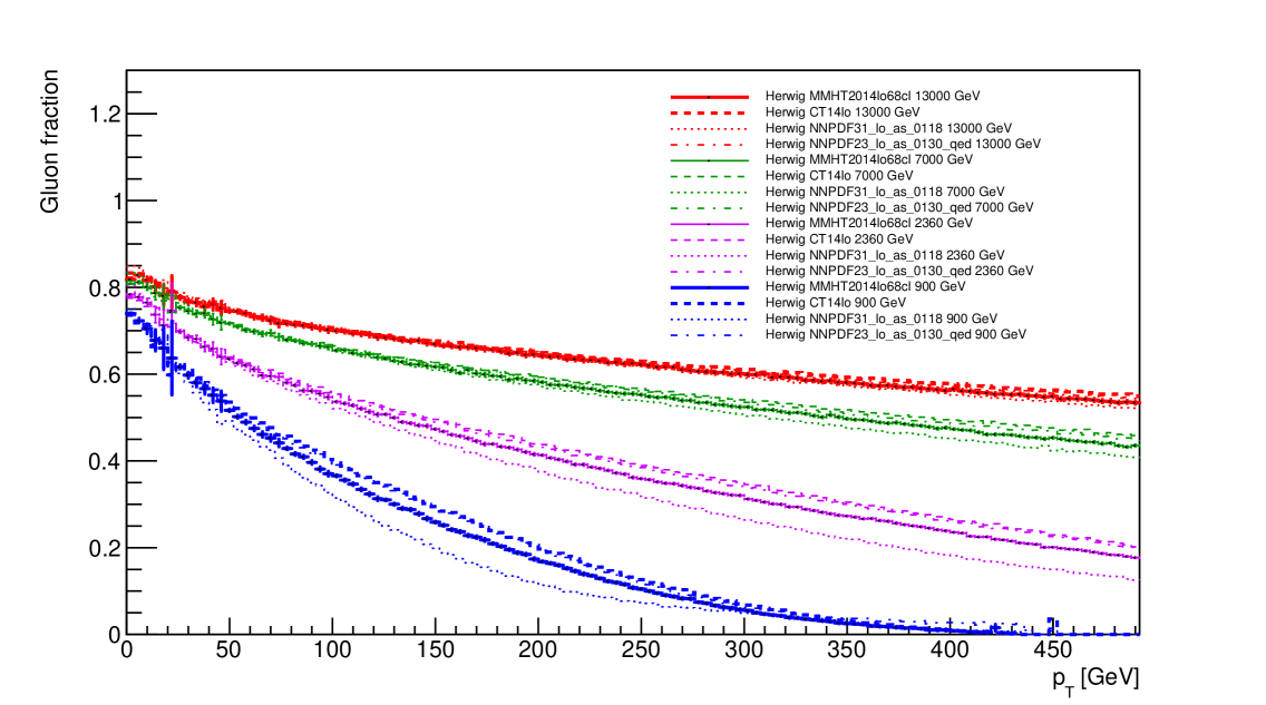
By disabling hadronization and parton showering in the Monte Carlo generators Herwig 7 and Pythia 8 the gluon fraction was defined as a function of
| (7) |
where represents the number of partons (quarks or gluons). In the left panel of Figure 1 we show examples of gluon fractions as a function of transverse momentum at GeV and GeV of Herwig (solid lines). We have also performed a more sophisticated approach with the distribution of gluon fractions as a 2D map in and pseudorapidity of a jet . However, no significant differences were observed in the resulting quark and gluon angularities. Therefore, for simplicity, the strategy of taking the mean of the jet distributions is used to obtain numerical results in the following sections.
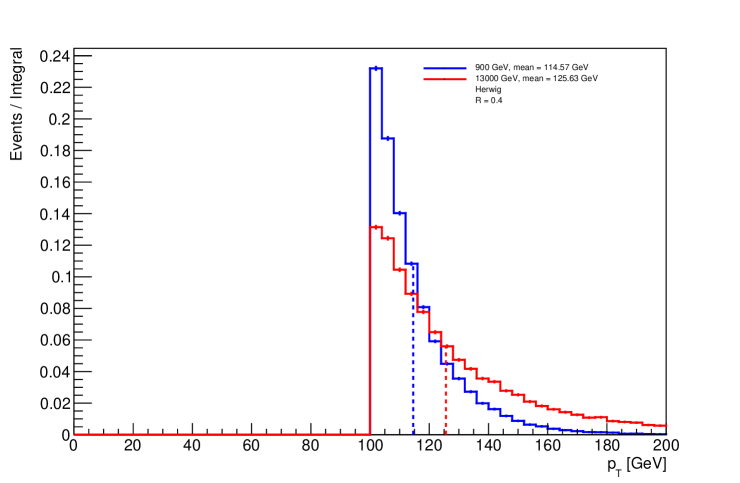
Step 2: Evaluate the scaling coefficients and
In the right panel of Figure 1 we show the distributions of jets () that passed the event selection cuts defined in Section 2.1 obtained by running a complete Monte Carlo simulation (including hadronization and parton shower) at two different collision energies and GeV. The transverse momentum mean of the jet distribution for the two energies is as follows:
-
•
jet ( GeV) GeV,
-
•
jet ( TeV) GeV.
The scaling coefficients and , as illustrated by the dashed lines in Fig. 1, are obtained using the gluon fractions of the left panel at the derived from the right panel of Figure 1:
| (8) | |||||
| (9) |
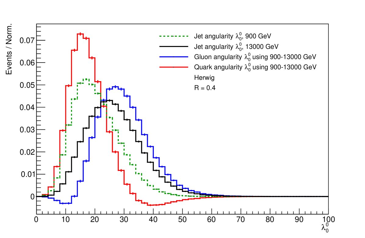
Step 3: Derive q/g angularities
Since jet angularities require the simulation of Monte Carlo events at the hadron level, we store them while generating the events needed to obtain the mean transverse momentum in Step 2. Then the jet angularities are normalised to the number of jets (entries of the distribution). An example of jet angularity (multiplicity) at 900 (green dashed line) and 13000 GeV (black solid line) is shown in Figure 2.
3 Robustness of observables to systematic effects
An important question to consider is whether the q/g angularities obtained in our study are robust to the impact of multiparton interactions (MPI) and initial state radiation (ISR). To address this, we performed supplementary Monte Carlo simulations for each observable examined, where we excluded the effects of MPI and ISR. This enabled us to evaluate the robustness of the q/g angularities obtained. Another crucial aspect to consider is the extent to which the q/g angularities remain independent of the energy. To test the energy independence, we use six possible energy combinations (, , , , , GeV) to derive angularities in the same way as described in the example 2.2. Therefore, there are in total 24 distributions (12 for quark and 12 for gluon jet angularities) that we need to analyse per plot.
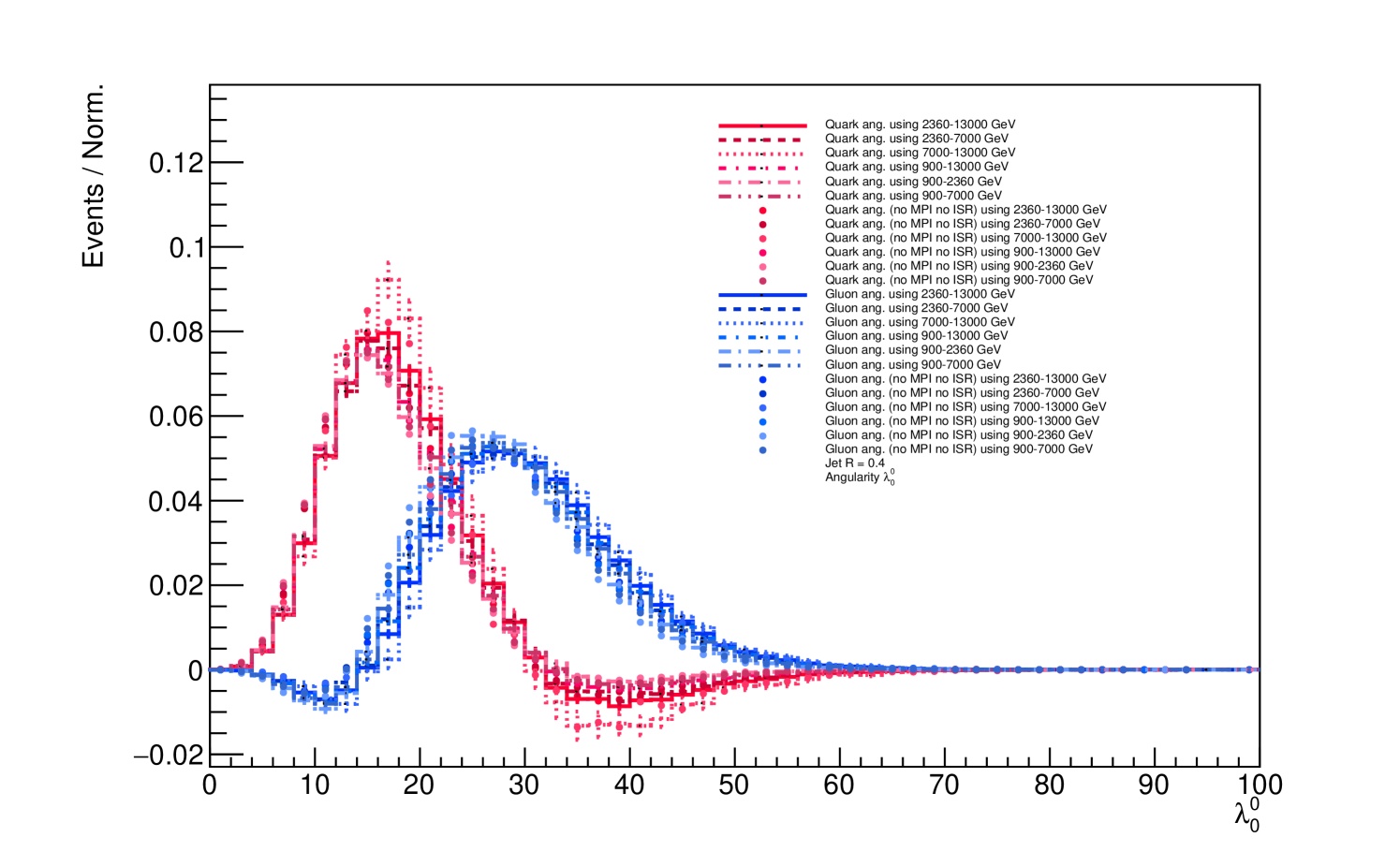
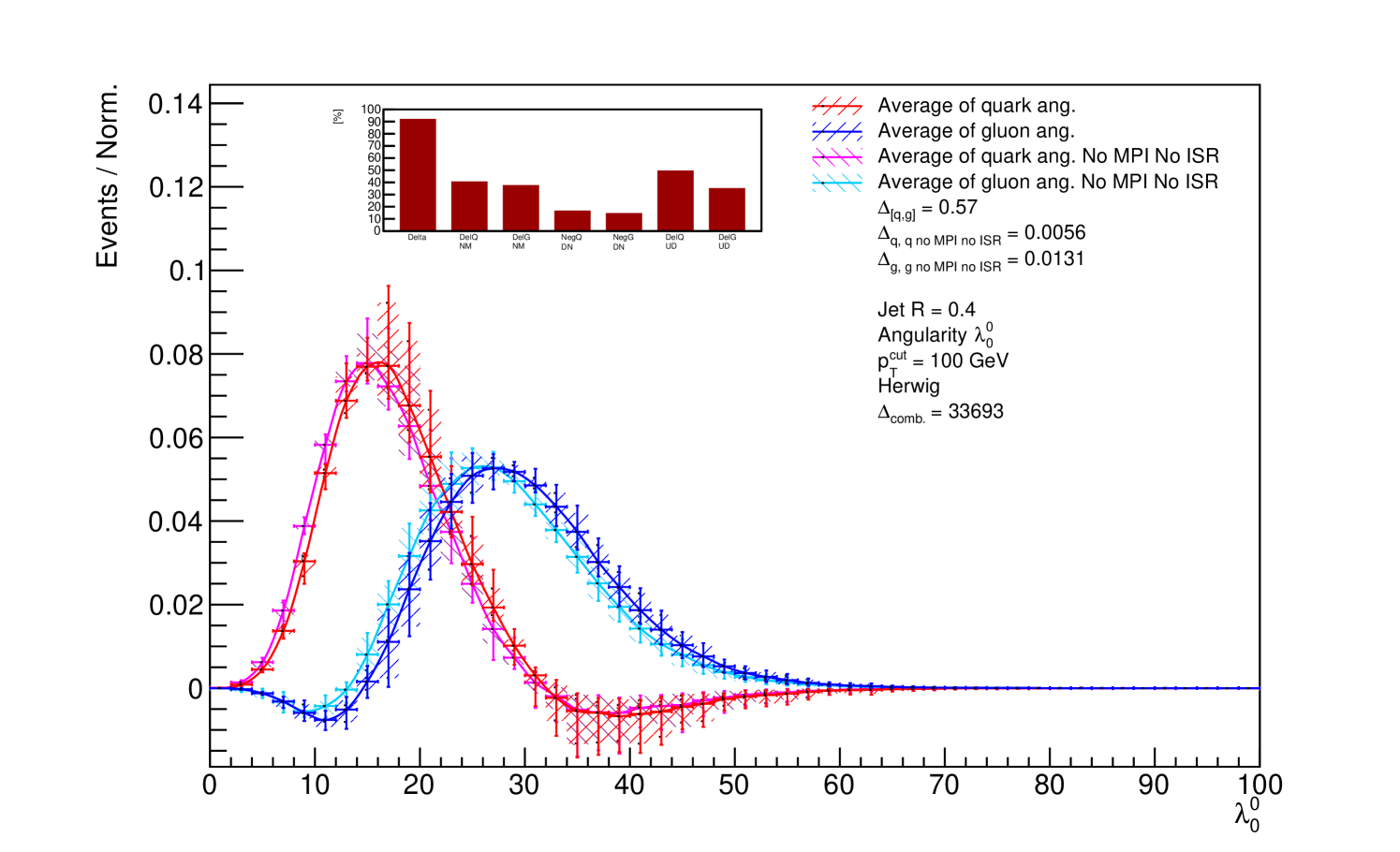
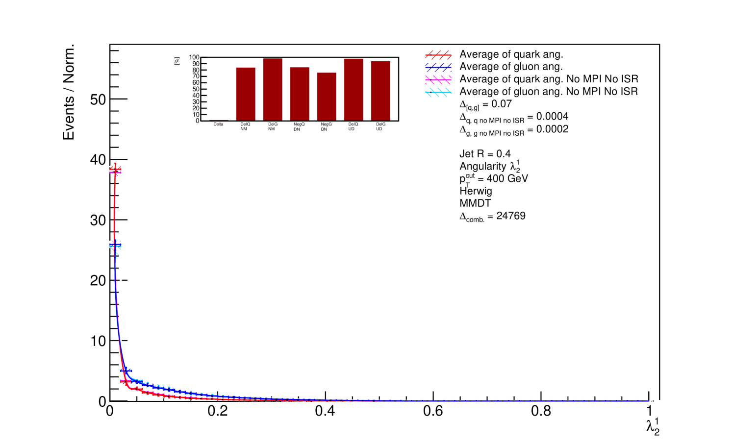
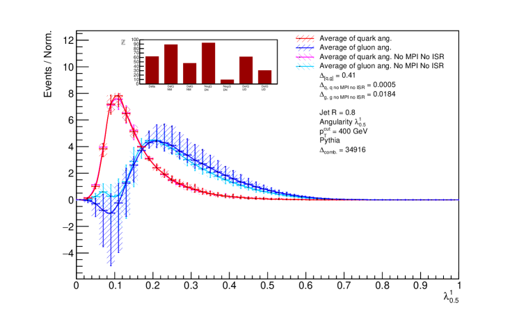
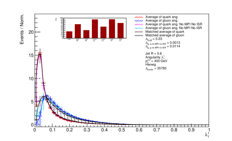
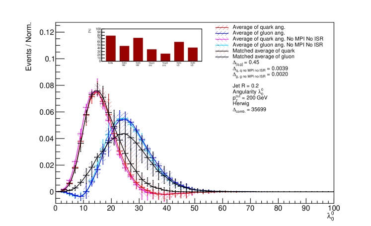
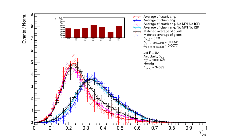
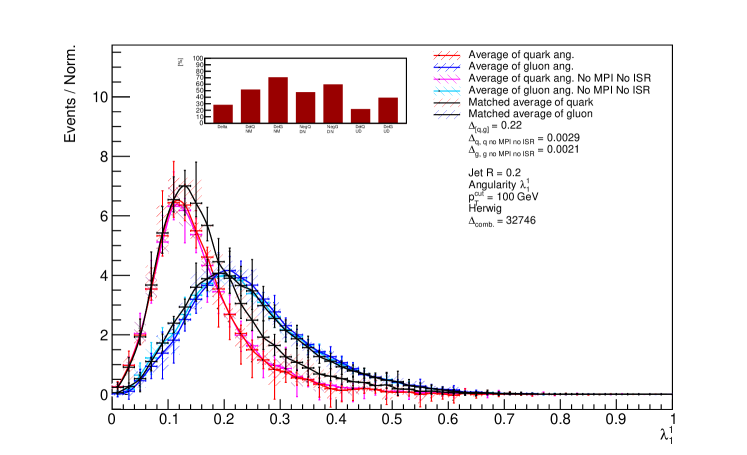
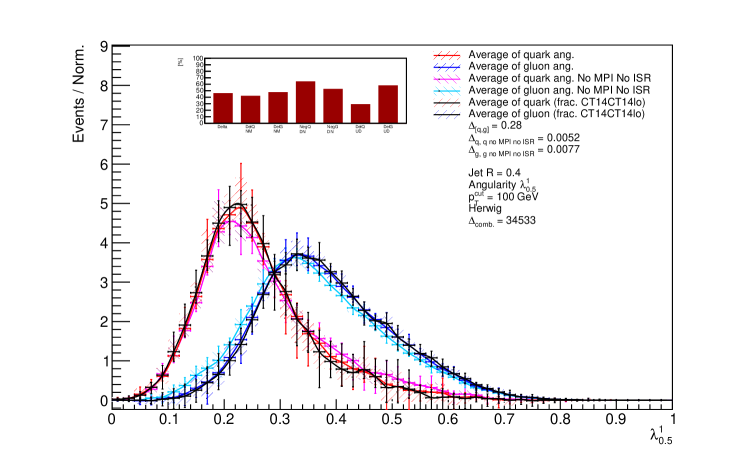
In the top panel of Figure 3 we present an example of this plot showing, similar to Figure 2, the multiplicity (, GeV) of the quark jets (red lines) and the gluon jets (blue lines). This time, the display includes angularities obtained from all energy combinations using full simulation, which are denoted by various types of lines. Additionally, the dots represent the angularities derived with MPI and ISR turned off. In order to simplify this plot, the bottom panel shows the same observable but this time solid lines represent the averaged q/g angularities across different energy combinations, while the filled area depicts the envelope of the different energy combinations, and the ticks represent the envelope of the statistical uncertainties of the angularities. By comparing this graph with Figure 2, we can gain additional insight into how the observables are robust to these important systematic effects. The averaging not only simplifies the detailed plots but also allows us to define measures (shown in the subhistogram with 7 bins), which help to sort angularities based on their performance. These measures are discussed in the next section.

4 Quantifying the quark/gluon separation power
Since we will be testing many variants of observables, we need a way to quantify the quark/gluon separation power in a robust way that can be easily summarised by a single number. For example, in Larkoski:2014pca , the authors quantify discrimination performance in the context of quark/gluon jets using classifier separation (a default output of the TMVA package 2007physics…3039H ):
| (12) |
Here denotes the number of bins, () is the -th bin content222As we saw earlier the resulting distributions can have negative bin values. This can lead to large values since the denominator can be equal to or close to zero. Therefore, in the case of negative bins in eq. 12, we set their value to zero. When the bin values for both quark and gluon angularities are equal to zero, these bins are neglected in the sum. of the probability distribution for the quark jet (gluon jet) sample as a function of the classifier . corresponds to no discrimination power (the distributions are exactly the same) while corresponds to perfect discrimination power.
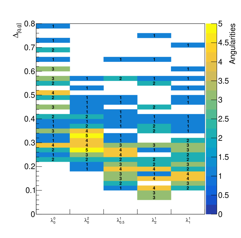
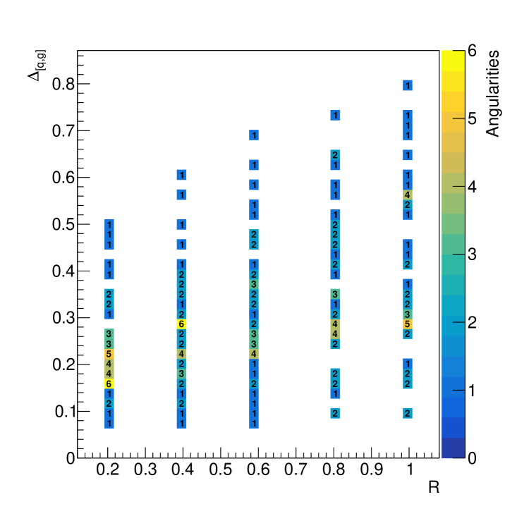
In Fig. 4 (left panel), we show the separation of the classifier as a function of the jet radius for all the energy-averaged angularities studied. We see that the separation power increases with increasing jet radius. This can be intuitively understood, since in larger jets more information about the radiation pattern is contained, which should be different for quark and gluon jets. Similarly, in Fig. 4 (right panel) we see that the separation power decreases with increasing . Finally, it is clear from Fig. 5 that although several individual cases of other angularities have high separation, it is multiplicity that scores the highest in most cases.
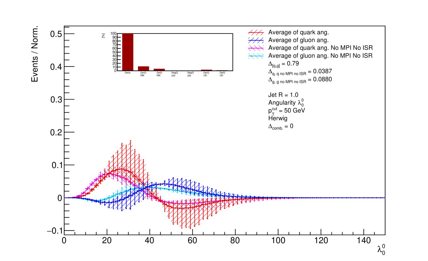
According to this measure, the best observable is the multiplicity with for GeV that is shown in Fig. 6.
As we can see from the figure, despite a large separation power, this observable suffers from various problems. First, it is not robust to MPI and ISR effects, and is also very energy dependent, which leads to unphysical negative bins of the probability distributions. For this reason, it is clear that this single measure is not suitable for our problem; therefore, we introduce additional measures to evaluate the robustness to the important systematic effects. To check the robustness of an observable to MPI and ISR effects, we calculated the separation power between the quark (gluon) angularity obtained with and without MPI and ISR i.e.: (). If these values are close to zero, then the observable is not sensitive to MPI and ISR effects. Similarly, to determine the extent to which the observable is energy independent, we calculated its separation power between the upper boundary and the lower boundary of the energy envelope of an angularity (see, for example, the energy envelope in Fig. 6). For quark (gluon) angularity, we denote this measure by () and its value close to zero means that the observable is energy independent. Finally, to measure whether the reconstructed observable suffers from the fact that part of it is negative, we calculate the percentage of negative area of down variation of the uncertainty band of quark (gluon) angularity and call it quark (gluon) negativity. We show the distributions of all of these measures in the Appendix (including repetition of Figs. 4 and 5 for completeness). We see that the MPI and ISR affect larger radius jets more than smaller (Fig. 41), as would be expected, and multiplicity much more than the other angularities (Fig. 42). Its effect gets somewhat less important at higher (Fig. 43). The energy-dependence shows a rather similar behaviour (Figs. 47–49), except that the smallest jet radius, 0.2, shows a strong dependence (Fig. 47). The energy-dependence of the multiplicity distributions is again strong (Fig. 48). A strong energy dependence or MPI and ISR dependence also leads to a significant amount of negativity in the distributions, and the negativity tends to follow these same patterns (Figs. 44–46).
Scores for a given observable of each metric, including , are shown as red columns in the subpad, see, for example, Figure 6. Each column represents the percentiles of a measure of angularities in all regions 50, 100, 200, and 400 GeV. The higher the column, the better the performance of the characteristic; for example, if the first column denoted by Delta in Figure 6 is the highest (100%) it means that no other angularity has a higher separation power . Similarly, if the other columns are high, it means that the corresponding measures are good, i.e. have low values. Successively, the columns from left to right show the percentiles of (1st column – Delta), the percentiles of and (2nd – DelQ NM and 3rd – DelG NM columns), the percentiles of quark and gluon negativity (4th – NegQ DN and 5th – NegG DN columns), the percentiles of and (6th - DelQ UD and 7th - DelG UD columns). From the subpanel of Fig. 6, we can read that the multiplicity with for GeV has the best separation power (1st column) but the fact that all other columns (2–7) are very low show that this is amongst the worst observables on these metrics. On the other hand, we can also have examples of observables that are very robust to all systematic effects, but have minimal separation power; see, for example, Fig.7. Therefore, in the next section, we will provide selections of plots which have strong robustness to systematic effects and have a high separation power.
5 Results
In studying these different observables, we have generated a huge number of distributions, since we consider all combinations of:
-
•
5 – angularities , , , ,
-
•
2 – using groomed (MMDT) / not groomed jets
-
•
5 – jet radii
-
•
4 – regions - dijet average GeV, 100, 200, and 400 GeV
-
•
2 – quark/gluon
-
•
2 – MPI and ISR switched on/off
-
•
6 – energy combinations: 900–2360, 900–7000, 900–13000, 2360–7000, 2360–13000, 7000–13000 GeV
-
•
2 – event generators Herwig and Pythia
This results in 200 plots for each of the two generators, each containing four distributions, each with an envelope of six different energy combinations, or 9600 distributions in total. Our aim is to sort through these to find the best performing combinations. Clearly to do so, we need a quantitative quality measure.
With the aim of picking the best candidates, maximising the separation power while also considering the other quality measures, we define the combined measure as:
| (13) |
where the power of three enhances the separation power . Each of the inputs into this formula is the percentile of the corresponding variable, i.e. the red bars in the inset. The addition of 1 is mainly only relevant to ensure that if a given observable is the worst on any single measure, it will be given an overall score of zero, and is otherwise unimportant. If there was one observable that was the best on every criterion, it would score the maximum possible value333Note that we do not ascribe any importance to the absolute value of , it is purely a means to rank the observables. of . We focus initially on the results from Herwig and return to the comparison with Pythia in the next section.
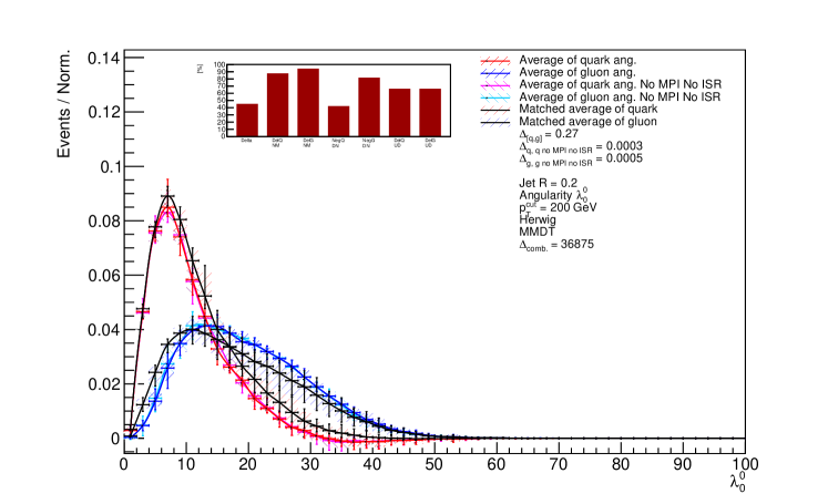
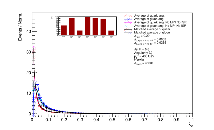
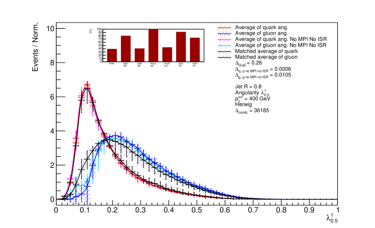
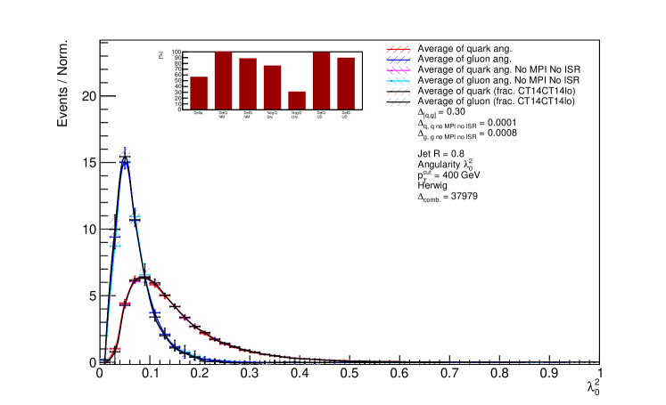
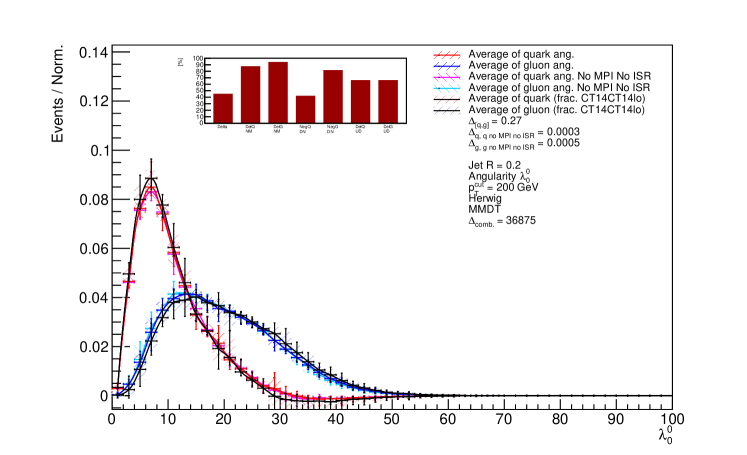
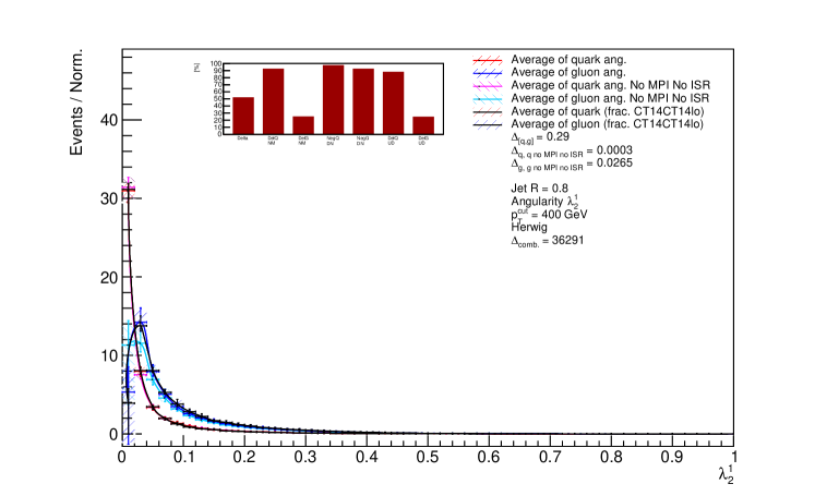
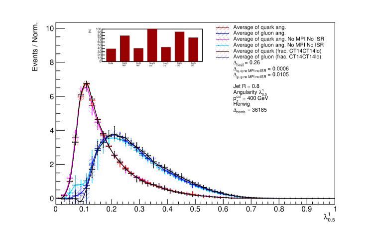
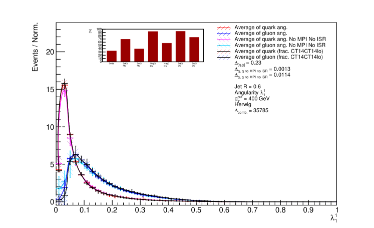
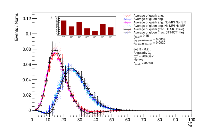
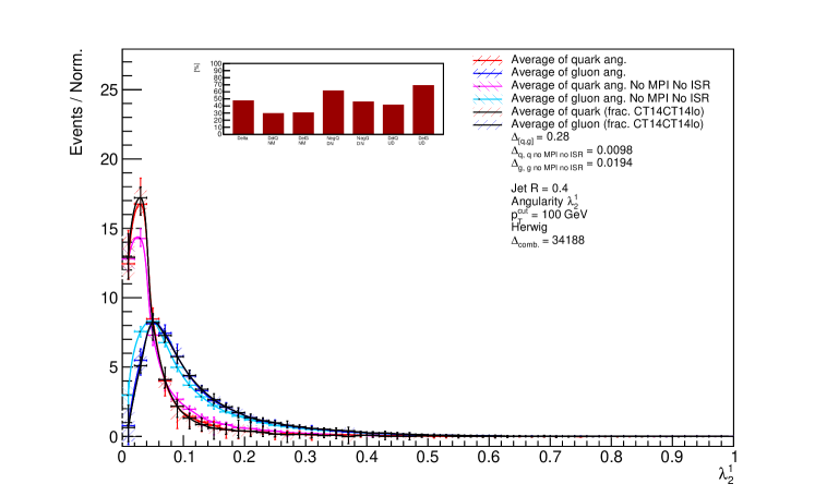
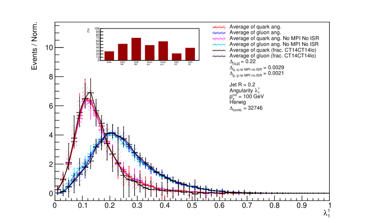
Figures 8, 9, 10, 11 and 12 represent the best selection based on score for each type of angularity.
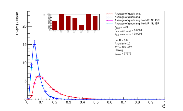
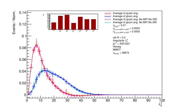
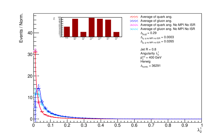
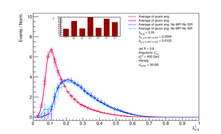
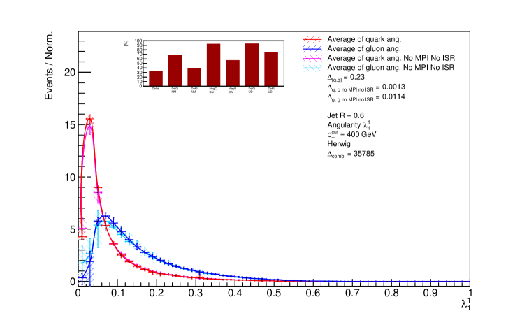
In addition to these best of each type, we have also selected four others, shown in Figures 13, 14, 15 and 16 based more on giving a representation of a typical range of good results, even though the score is not the highest. They generally show a good quark/gluon jet separation, even if they suffer from lower robustness to variations without MPI and ISR or negativity, etc.
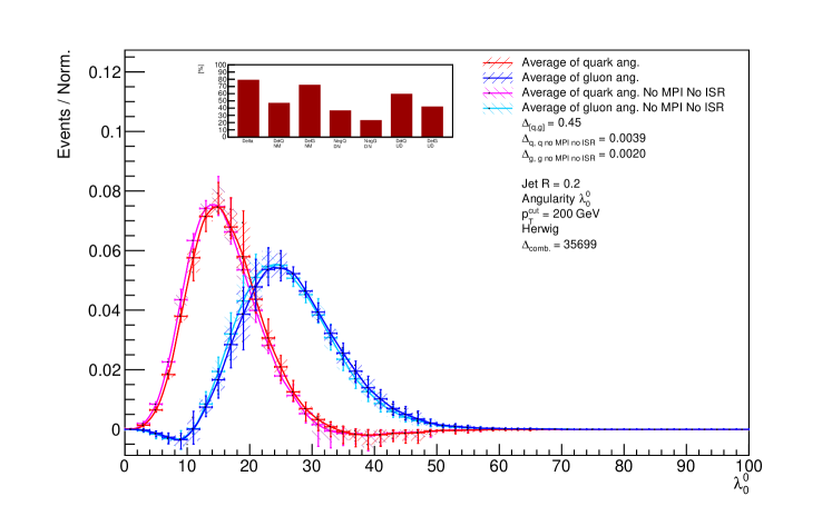
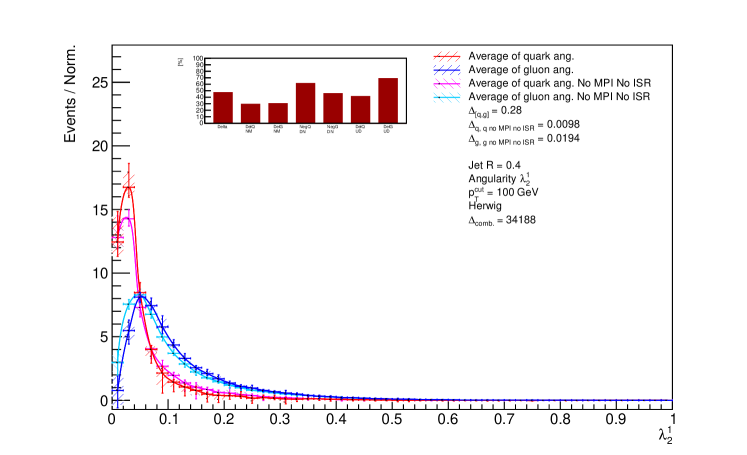
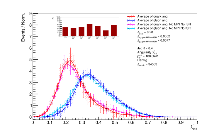
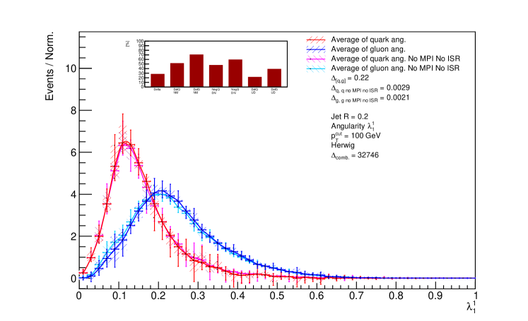
The high-scored angularities presented in the plots provide compelling evidence supporting the assumption that quark and gluon angularities remain independent of collision energy. This conclusion is drawn from the relatively narrow envelope of the filled area, which represents angularities derived at different energy combinations. The consistency observed across these plots strongly suggests that quark and gluon angularities are not significantly affected by changes in collision energy. However, it is essential to acknowledge that this assumption may not be entirely valid for all angularities, as shown in Figure 6 where the filled area is broader. Therefore, it is important to consider this uncertainty when interpreting the results.
5.1 Comparison with Pythia
We have rerun the preceding analysis using the Pythia event generator in place of Herwig. The results are very similar in almost all cases. As an example, we show the angularity that has the highest score in Figure 17.

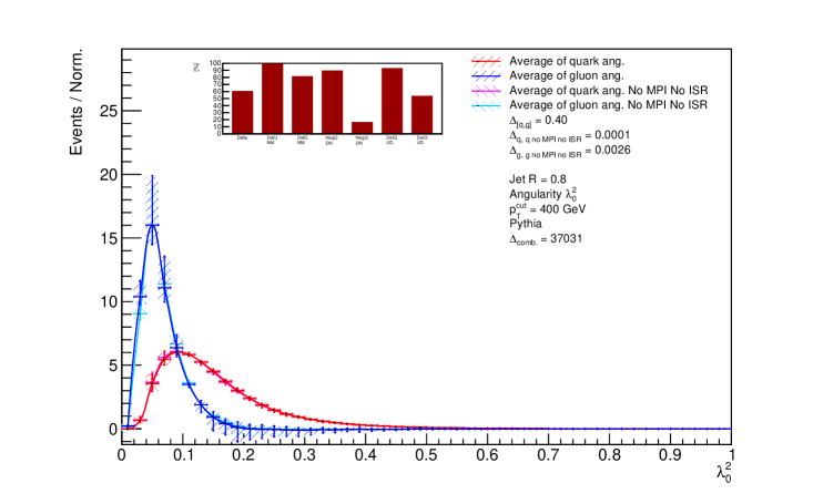
We also show, in Figure 18, the example from all those we have studied that shows the biggest difference between Herwig and Pythia.
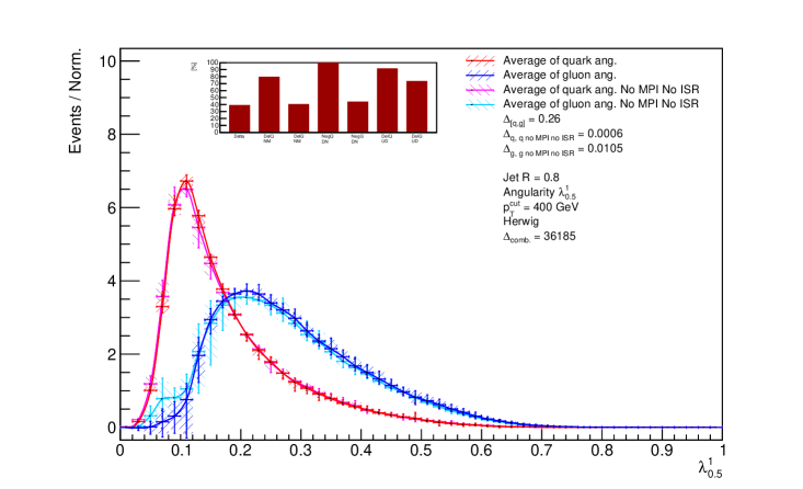
In general, and most noticeably in Fig. 18, Pythia shows slightly more energy- and MPI/ISR-dependence than Herwig, and as a result slightly more negativity. Although for most of the robust observables this is a small effect, it is possible that it could also be used to constrain the underlying models, by studying observables where it is significant.
6 Conclusion
We have shown that several jet angularity observables can be robust in measuring the properties of jets and successful in yielding significantly different distributions for quark and gluon jets. And, moreover, that the energy-dependence of the distributions can be used at the LHC to separate the two on a statistical basis. The method relies crucially on the assumption that the angularities for quark and gluon jets are separately independent of , and we have shown this to be the case, particularly for higher jets. Only for multiplicity in large-radius jets are the uncertainties too high to be useful.
Of course, the LHC will not make special runs at different energies only to conduct the proposed measurement. Therefore, we should use data already recorded, or data that will soon be measured at the LHC. During its early startup phase, CMS recorded some minimum-bias events of proton-proton collisions at energies GeV and GeV. In the publication CMS:2010bva , they presented properties of inclusive jets and dijet events measured in these samples. However, the number of events with jet GeV or GeV was less then or , at GeV and GeV respectively. Due to the low statistics and the low jet cut, these data samples are not optimal for using our method. For this reason, carrying out the proposed measurement at the LHC at energies of and TeV, where low statistics will not be an issue, would be a much better strategy. It is also worth mentioning that the ALICE experiment has also measured jets at energies GeV and TeV. Jet measurements at these energies and in particular at TeV where the number of jets measured is high could serve to check the energy independence of the quark/gluon jet measurement. Moreover, recently ALICE published results ALICE:2021njq ; Lesser:2022lpc of jet substructure including jet angularities carried out by the experiment using data recorded at the LHC from pp collisions at or TeV. It is possible that these data could be reanalysed to obtain the first results using the method proposed here. Another possibility could be to use CERN Open Data CERNopenData similarly to what was done for jet topics Komiske:2022vxg .
One interesting extension of this research would be to use the recently developed IRC-safe flavoured jet algorithms Caletti:2022glq ; Banfi:2006hf ; Caletti:2022hnc ; Czakon:2022wam ; Gauld:2022lem ; Caola:2023wpj . Knowing the flavour of jets could be used to construct the fraction of jets after the evolution of the parton shower, which could help to trace the origin of the jets through hadronisation and parton showering, and finally be used to develop a Machine Learning method to optimise the q/g classification strategy. Another interesting extension would be to study different jet production processes, such as vector boson plus jet, at different collision energies. Not only is the flavour mix different in these processes, but also the colour structure. Yet another intriguing possibility would be to apply the variable collision energy samples to the above-mentioned jet topics.
Acknowledgements
MS gratefully acknowledges funding from the UK Science and Technology Facilities Council (grant number ST/T001038/1). The work of AS and PB is funded by grant no. 2019/34/E/ST2/00457 of the National Science Centre, Poland. PB is also supported by the Priority Research Area Digiworld under the program Excellence Initiative – Research University at the Jagiellonian University in Cracow and by the Polish National Agency for Academic Exchange NAWA under the Programme STER Internationalisation of doctoral schools, Project no. PPI/STE/2020/1/00020.
7 Appendix
7.1 Comparison against “truth level” distributions
In this section, we compare the quark and gluon distributions we extract against “truth level” distributions, which are shown as the black lines. We obtain these by assigning each reconstructed jet the flavour of the hard parton to which it is closest in direction (smallest ). We see that for our most robust angularities, there is very good agreement, while for the distributions that have significant energy-dependence or negativity, the agreement is poorer.


7.2 Fractions using different PDF sets
We have studied the PDF dependence of our results by comparing the results extracted using the gluon fractions from the NNPDF23 LO QED with Ball:2013hta , NNPDF31 LO with NNPDF:2017mvq and CT14lo Dulat:2015mca sets and find generally very small differences. In this section, we illustrate this for the CT14lo PDF set, which gives the results plotted by black lines over our default results in red and blue.
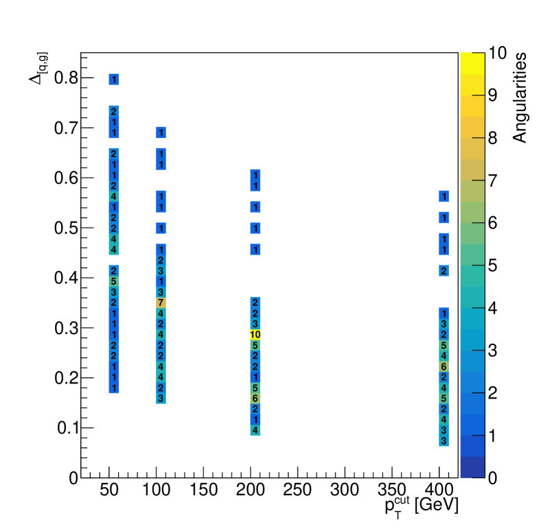
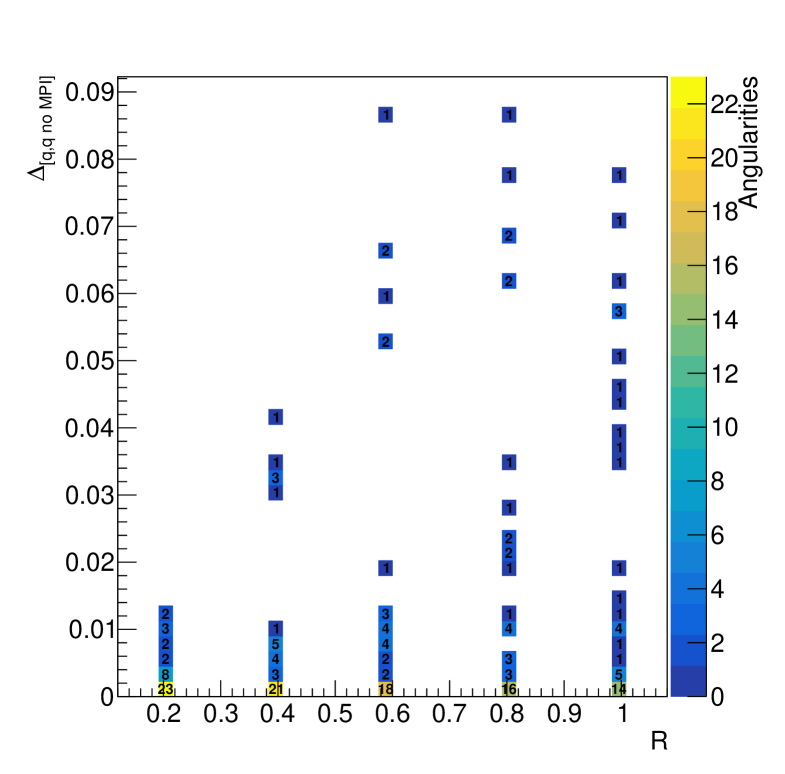
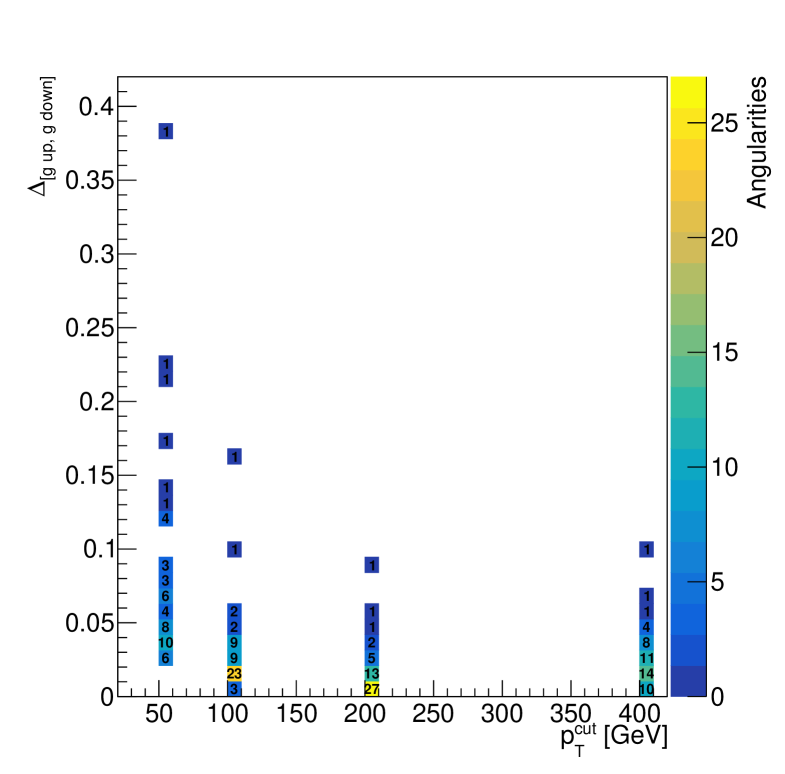
7.3 Scatter Plots
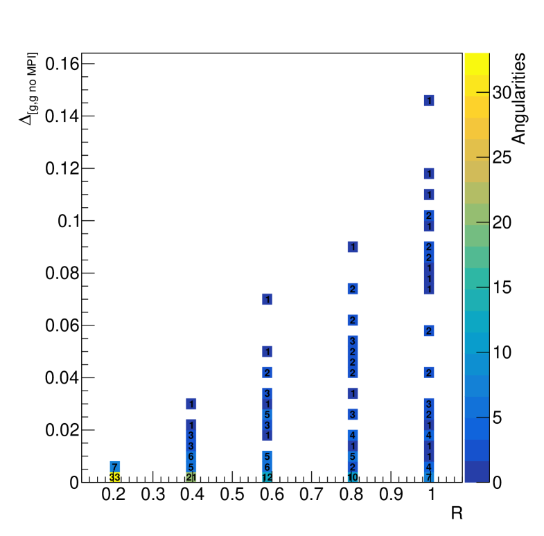
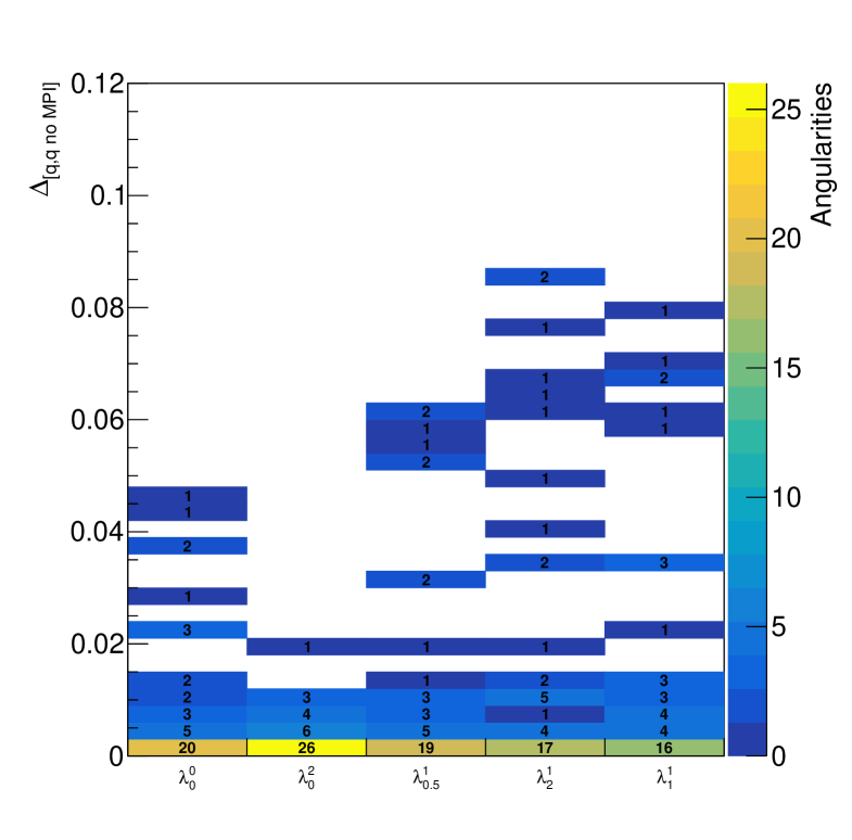
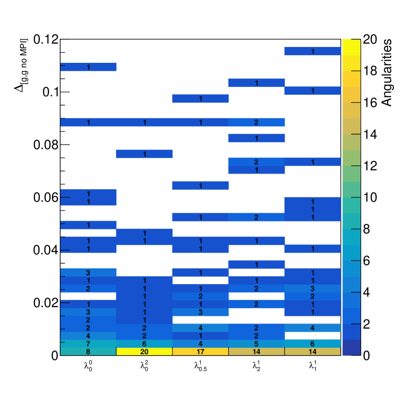
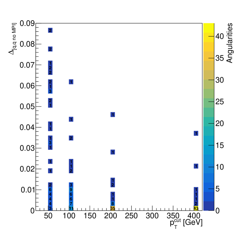
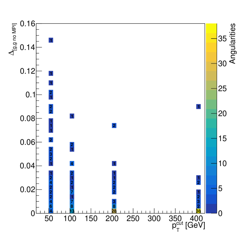
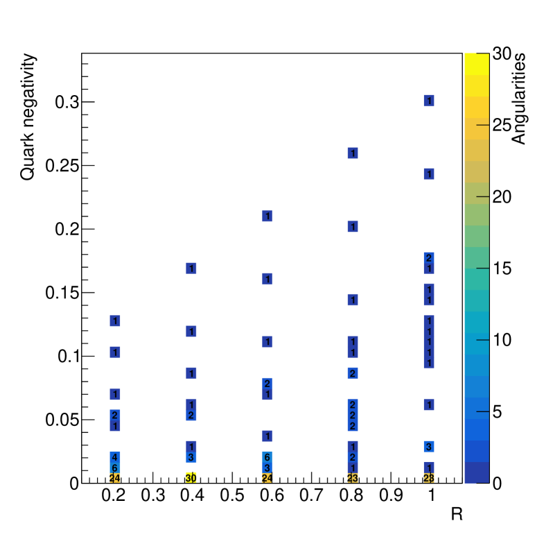
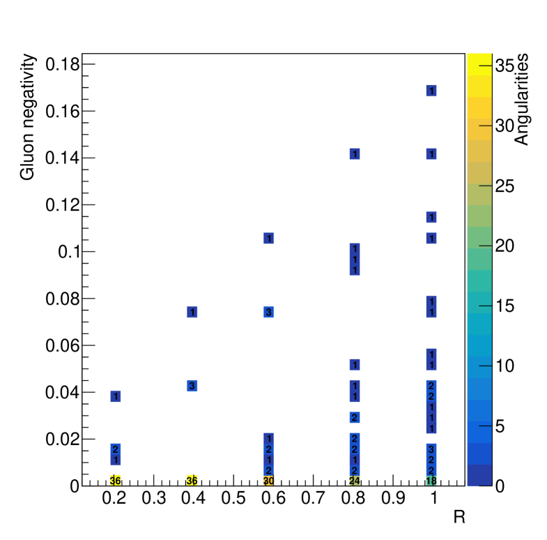
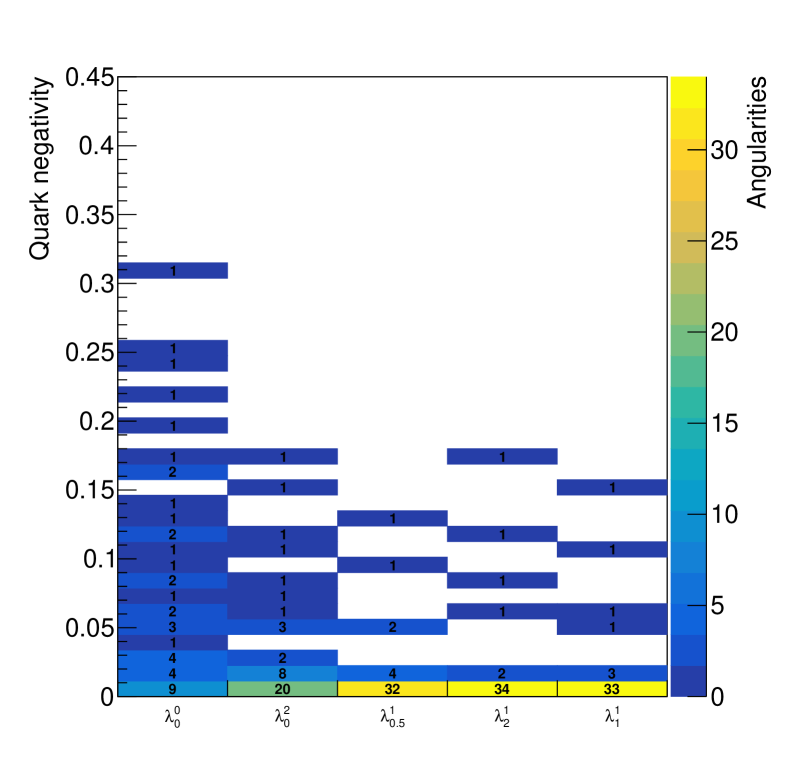
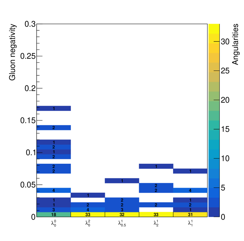
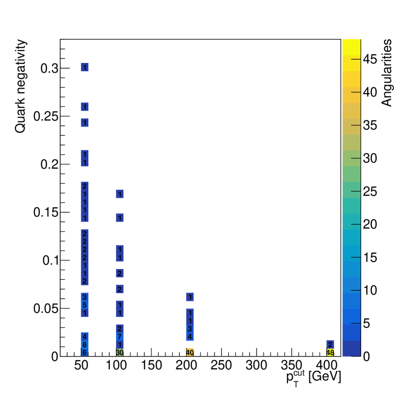
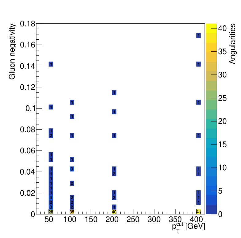
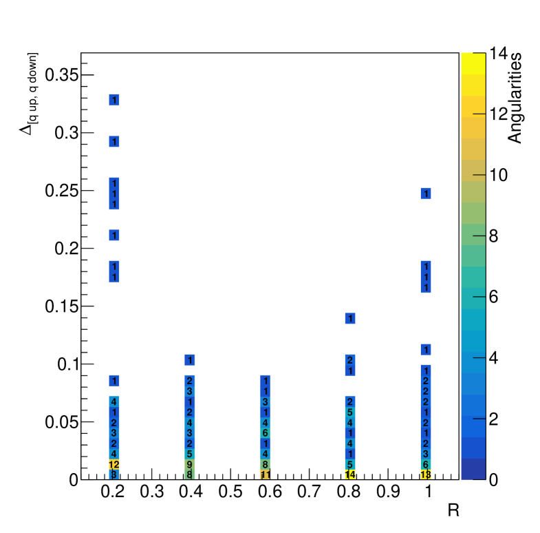
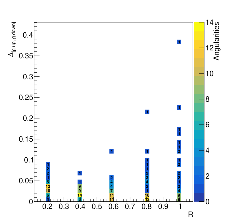
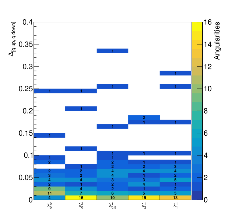
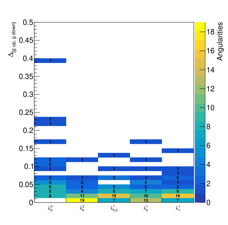
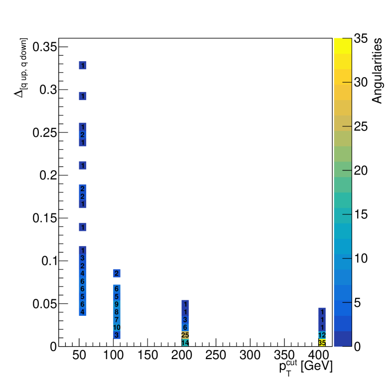
In this appendix, we show scatter plots of the absolute values of the measures , and , quark and gluon negativity, and as functions of radius , angularities, and jet . The columns in the subpad of the results plots of quark and gluon angularities are calculated as percentiles of these absolute values.


References
- (1) J. Gallicchio and M. D. Schwartz, Quark and Gluon Tagging at the LHC, Phys. Rev. Lett. 107 (2011) 172001, [1106.3076].
- (2) D. Ferreira de Lima, P. Petrov, D. Soper and M. Spannowsky, Quark-Gluon tagging with Shower Deconstruction: Unearthing dark matter and Higgs couplings, Phys. Rev. D 95 (2017) 034001, [1607.06031].
- (3) B. Whitmore, Search for Beyond the Standard Model signals in a quark-gluon tagged dijet final state with the ATLAS detector. PhD thesis, Lancaster U. (main), 2019. 10.17635/lancaster/thesis/738.
- (4) B. Bhattacherjee, S. Mukhopadhyay, M. M. Nojiri, Y. Sakaki and B. R. Webber, Quark-gluon discrimination in the search for gluino pair production at the LHC, JHEP 01 (2017) 044, [1609.08781].
- (5) H. T. Li, B. Yan and C. P. Yuan, Discriminating between Higgs Production Mechanisms via Jet Charge at the LHC, Phys. Rev. Lett. 131 (2023) 041802, [2301.07914].
- (6) X. Wong and B. Yan, Probing the coupling through the jet charge correlation in Higgs boson decay, 2302.02084.
- (7) J. Gallicchio and M. D. Schwartz, Quark and Gluon Jet Substructure, JHEP 04 (2013) 090, [1211.7038].
- (8) Y. Sakaki, Quark jet rates and quark-gluon discrimination in multijet final states, Phys. Rev. D 99 (2019) 114012, [1807.01421].
- (9) Z. Fodor, How to See the Differences Between Quark and Gluon Jets, Phys. Rev. D41 (1990) 1726.
- (10) J. Pumplin, How to tell quark jets from gluon jets, Phys. Rev. D44 (1991) 2025–2032.
- (11) I. W. Stewart and X. Yao, Pure quark and gluon observables in collinear drop, JHEP 09 (2022) 120, [2203.14980].
- (12) E. M. Metodiev and J. Thaler, Jet Topics: Disentangling Quarks and Gluons at Colliders, Phys. Rev. Lett. 120 (2018) 241602, [1802.00008].
- (13) C. Frye, A. J. Larkoski, J. Thaler and K. Zhou, Casimir Meets Poisson: Improved Quark/Gluon Discrimination with Counting Observables, JHEP 09 (2017) 083, [1704.06266].
- (14) J. Davighi and P. Harris, Fractal based observables to probe jet substructure of quarks and gluons, Eur. Phys. J. C 78 (2018) 334, [1703.00914].
- (15) D. Goncalves, F. Krauss and R. Linten, Distinguishing b-quark and gluon jets with a tagged b-hadron, Phys. Rev. D 93 (2016) 053013, [1512.05265].
- (16) F. A. Dreyer, G. Soyez and A. Takacs, Quarks and gluons in the Lund plane, JHEP 08 (2022) 177, [2112.09140].
- (17) S. Bright-Thonney and B. Nachman, Investigating the Topology Dependence of Quark and Gluon Jets, JHEP 03 (2019) 098, [1810.05653].
- (18) B. Bhattacherjee, S. Mukhopadhyay, M. M. Nojiri, Y. Sakaki and B. R. Webber, Associated jet and subjet rates in light-quark and gluon jet discrimination, JHEP 04 (2015) 131, [1501.04794].
- (19) P. T. Komiske, E. M. Metodiev and J. Thaler, An operational definition of quark and gluon jets, JHEP 11 (2018) 059, [1809.01140].
- (20) P. T. Komiske, S. Kryhin and J. Thaler, Disentangling quarks and gluons in CMS open data, Phys. Rev. D 106 (2022) 094021, [2205.04459].
- (21) P. Gras, S. Höche, D. Kar, A. Larkoski, L. Lönnblad, S. Plätzer et al., Systematics of quark/gluon tagging, JHEP 07 (2017) 091, [1704.03878].
- (22) D. Reichelt, P. Richardson and A. Siodmok, Improving the Simulation of Quark and Gluon Jets with Herwig 7, Eur. Phys. J. C77 (2017) 876, [1708.01491].
- (23) A. Siódmok, Quark/Gluon Jets Discrimination and Its Connection to Colour Reconnection, Acta Phys. Polon. B 48 (2017) 2341.
- (24) ATLAS collaboration, G. Aad et al., Light-quark and gluon jet discrimination in collisions at with the ATLAS detector, Eur. Phys. J. C 74 (2014) 3023, [1405.6583].
- (25) CMS, ATLAS collaboration, R. Aggleton, Measurements of jet substructure in quark and gluon jets, Nucl. Part. Phys. Proc. 312-317 (2021) 1–5.
- (26) M. H. Seymour, The Average number of subjets in a hadron collider jet, Nucl. Phys. B 421 (1994) 545–564.
- (27) M. W. Krasny, F. Fayette, W. Placzek and A. Siodmok, Z-boson as ’the standard candle’ for high precision W-boson physics at LHC, Eur. Phys. J. C51 (2007) 607–617, [hep-ph/0702251].
- (28) M. W. Krasny, F. Dydak, F. Fayette, W. Placzek and A. Siodmok, at the LHC: a forlorn hope?, Eur. Phys. J. C 69 (2010) 379–397, [1004.2597].
- (29) F. Fayette, M. W. Krasny, W. Placzek and A. Siodmok, Measurement of at LHC, Eur. Phys. J. C 63 (2009) 33–56, [0812.2571].
- (30) M. L. Mangano and J. Rojo, Cross Section Ratios between different CM energies at the LHC: opportunities for precision measurements and BSM sensitivity, JHEP 08 (2012) 010 [1206.3557].
- (31) D0 collaboration, Subjet multiplicity in quark and gluon jets at D0, in 20th International Symposium on Lepton and Photon Interactions at High Energies (LP 01), 6, 2001. hep-ex/0106040.
- (32) D0 collaboration, V. M. Abazov et al., Subjet Multiplicity of Gluon and Quark Jets Reconstructed with the Algorithm in Collisions, Phys. Rev. D 65 (2002) 052008, [hep-ex/0108054].
- (33) OPAL collaboration, G. Alexander et al., A Direct observation of quark - gluon jet differences at LEP, Phys. Lett. B 265 (1991) 462–474.
- (34) CMS collaboration, A. Tumasyan et al., Study of quark and gluon jet substructure in Z+jet and dijet events from pp collisions, JHEP 01 (2022) 188, [2109.03340].
- (35) J. R. Forshaw and M. H. Seymour, Subjet rates in hadron collider jets, JHEP 09 (1999) 009, [hep-ph/9908307].
- (36) A. J. Larkoski, J. Thaler and W. J. Waalewijn, Gaining (Mutual) Information about Quark/Gluon Discrimination, JHEP 11 (2014) 129, [1408.3122].
- (37) F. Pandolfi and D. Del Re, Search for the Standard Model Higgs Boson in the Decay Channel at CMS. PhD thesis, Zurich, ETH, 2012.
- (38) CMS collaboration, S. Chatrchyan et al., Search for a Higgs boson in the decay channel to ZZ(*) to qbar l+ in collisions at TeV, JHEP 04 (2012) 036, [1202.1416].
- (39) J. R. Andersen et al., Les Houches 2015: Physics at TeV Colliders Standard Model Working Group Report, in 9th Les Houches Workshop on Physics at TeV Colliders (PhysTeV 2015) Les Houches, France, June 1-19, 2015, 2016. 1605.04692.
- (40) S. Catani, G. Turnock and B. R. Webber, Jet broadening measures in annihilation, Phys. Lett. B295 (1992) 269–276.
- (41) P. E. L. Rakow and B. R. Webber, Transverse Momentum Moments of Hadron Distributions in QCD Jets, Nucl. Phys. B191 (1981) 63.
- (42) R. K. Ellis and B. R. Webber, QCD Jet Broadening in Hadron Hadron Collisions, Conf. Proc. C860623 (1986) 74.
- (43) E. Farhi, A QCD Test for Jets, Phys. Rev. Lett. 39 (1977) 1587–1588.
- (44) J. Bellm et al., Herwig 7.0/Herwig++ 3.0 release note, Eur. Phys. J. C76 (2016) 196, [1512.01178].
- (45) J. Bellm et al., Herwig 7.2 release note, Eur. Phys. J. C 80 (2020) 452, [1912.06509].
- (46) L. A. Harland-Lang, A. D. Martin, P. Motylinski and R. S. Thorne, Parton distributions in the LHC era: MMHT 2014 PDFs, Eur. Phys. J. C 75 (2015) no.5, 204, [1412.3989].
- (47) T. Sjöstrand, S. Ask, J. R. Christiansen, R. Corke, N. Desai, P. Ilten et al., An Introduction to PYTHIA 8.2, Comput. Phys. Commun. 191 (2015) 159–177, [1410.3012].
- (48) C. Bierlich et al., A comprehensive guide to the physics and usage of PYTHIA 8.3, 2203.11601.
- (49) R. D. Ball et al. [NNPDF], Parton distributions with QED corrections, Nucl. Phys. B 877 (2013) 290-320, 1308.0598.
- (50) M. Cacciari, G. P. Salam and G. Soyez, The Anti-k(t) jet clustering algorithm, JHEP 04 (2008) 063, [0802.1189].
- (51) M. Cacciari and G. P. Salam, Dispelling the myth for the jet-finder, Phys. Lett. B 641 (2006) 57–61, [hep-ph/0512210].
- (52) M. Cacciari, G. P. Salam and G. Soyez, FastJet User Manual, Eur. Phys. J. C72 (2012) 1896, [1111.6097].
- (53) J. M. Butterworth, A. R. Davison, M. Rubin and G. P. Salam, Jet substructure as a new Higgs search channel at the LHC, Phys. Rev. Lett. 100 (2008) 242001, [0802.2470].
- (54) S. D. Ellis, C. K. Vermilion and J. R. Walsh, Techniques for improved heavy particle searches with jet substructure, Phys. Rev. D80 (2009) 051501, [0903.5081].
- (55) S. D. Ellis, C. K. Vermilion and J. R. Walsh, Recombination Algorithms and Jet Substructure: Pruning as a Tool for Heavy Particle Searches, Phys. Rev. D81 (2010) 094023, [0912.0033].
- (56) D. Krohn, J. Thaler and L.-T. Wang, Jet Trimming, JHEP 02 (2010) 084, [0912.1342].
- (57) M. Dasgupta, A. Fregoso, S. Marzani and G. P. Salam, Towards an understanding of jet substructure, JHEP 09 (2013) 029, [1307.0007].
- (58) A. J. Larkoski, S. Marzani, G. Soyez and J. Thaler, Soft Drop, JHEP 05 (2014) 146, [1402.2657].
- (59) A. Hoecker, P. Speckmayer, J. Stelzer, J. Therhaag, E. von Toerne, H. Voss et al., TMVA - Toolkit for Multivariate Data Analysis, ArXiv Physics e-prints (Mar., 2007) , [physics/0703039].
- (60) CMS collaboration, Jets in 0.9 and 2.36 TeV pp Collisions, tech. rep., CERN, Geneva, 2010. https://cds.cern.ch/record/1248210.
- (61) S. Acharya et al., ALICE collaboration, Measurements of the groomed and ungroomed jet angularities in pp collisions at = 5.02 TeV, JHEP 05 (2022) 061, [2107.11303].
- (62) ALICE collaboration, E. Lesser, Jet substructure in pp collisions with ALICE, in 56th Rencontres de Moriond on QCD and High Energy Interactions , 5, 2022. 2205.11583.
- (63) CERN open data. https://opendata.cern.ch/.
- (64) S. Caletti, A. J. Larkoski, S. Marzani and D. Reichelt, A fragmentation approach to jet flavor, JHEP 10 (2022) 158, [2205.01117].
- (65) A. Banfi, G. P. Salam and G. Zanderighi, Infrared safe definition of jet flavor, Eur. Phys. J. C47 (2006) 113–124, [hep-ph/0601139].
- (66) S. Caletti, A. J. Larkoski, S. Marzani and D. Reichelt, Practical jet flavour through NNLO, Eur. Phys. J. C 82 (2022) 632, [2205.01109].
- (67) M. Czakon, A. Mitov and R. Poncelet, Infrared-safe flavoured anti-kT jets, JHEP 04 (2023) 138, [2205.11879].
- (68) R. Gauld, A. Huss and G. Stagnitto, Flavor Identification of Reconstructed Hadronic Jets, Phys. Rev. Lett. 130 (2023) 161901, [2208.11138].
- (69) F. Caola, R. Grabarczyk, M. L. Hutt, G. P. Salam, L. Scyboz and J. Thaler, Flavoured jets with exact anti- kinematics and tests of infrared and collinear safety, 2306.07314.
- (70) R. D. Ball et al. [NNPDF], Parton distributions from high-precision collider data, Eur. Phys. J. C 77 (2017) no.10, 663, [1706.00428].
- (71) S. Dulat, T. J. Hou, J. Gao, M. Guzzi, J. Huston, P. Nadolsky, J. Pumplin, C. Schmidt, D. Stump and C. P. Yuan, New parton distribution functions from a global analysis of quantum chromodynamics, Phys. Rev. D 93 (2016) no.3, 033006, [1506.07443].