Novel traversable wormhole in General Relativity and Einstein-Scalar-Gauss-Bonnet theory supported by nonlinear electrodynamics
Abstract
Several traversable wormholes (T-WHs) of the Morris-Thorne type have been presented as exact solutions of Einstein-nonlinear electrodynamics gravity (GR-NLED), e.g. Arellano ; Bronnikov2017 ; Bronnikov_Walia ; Canate_Breton ; Canate_Breton_Ortiz ; Canate_Magos_Breton . However, none of these solutions is support by a nonlinear electrodynamics model satisfying plausible conditions. In this work, we present the first traversable wormhole solution of Einstein-nonlinear electrodynamics gravity coupled to a self-interacting phantom scalar field (GR-NLED-SF) with a NLED model such that in the limit of weak field becomes the Maxwell electrodynamics, is presented. Furthermore, we show that this novel T-WH spacetime is also an exact solution of the Einstein-scalar-Gauss-Bonnet (EsGB) theory with a nonlinear electrodynamics source, but now with a real scalar field having a positive kinetic term.
pacs:
04.20.Jb, 04.50.Kd, 04.50.-h, 04.40.NrI Introduction
The wormholes are fascinating predictions arising from the geometrical description of gravity. They involve a topological spacetime configuration as a shortcut between distant points or regions in spacetime. The first wormhole interpretation originally came from the work of Einstein and Rosen in 1935, with their solution known as the Einstein-Rosen bridge einstein35 , which is, in essence, the maximally extended Schwarzschild black hole solution kruskal60 . However, the “throat” of this wormhole is dynamic and hence non-traversable, meaning that its radius expands to a maximum and quickly contracts to zero so fast that even a photon cannot pass through kruskal60 .
Further, in 1988, a solution to the wormhole traversability problem was established by Morris and Thorne morris88 . They obtained one type of wormhole metric and the necessary conditions (absence of horizons and the flare-out condition) that can guarantee the traversability of a wormhole spacetime.
Moreover, they showed that in the context of general relativity (GR), the throat of these types of wormholes only could be kept open by some form of “exotic” matter morris88-2 having negative energy density and whose energy-momentum tensor violates the null-energy condition (NEC).
This kind of exotic fields have been intensely discussed,
principally, in the context of electromagnetic and scalar fields
Gibbons1996 .
Although an explanation about the fundamental origin of phantom fields
is still in discussion, they are frequently used, for instance;
in the construction of novel
cosmological models known as Phantom Cosmologies Pha_Cos ; Ph_SF1 ; Ph_SF .
Also, they have been used to explain the current period of accelerated expansion
of the Universe.
Indeed, an accelerated expansion of the Universe can be accounted
by assuming
the existence of an effective field generating repulsive gravity between its
elements,
e.g., a repulsive field would correspond in Einstein gravity to a fluid with negative pressure,
like dark energy, which is an essential ingredient of the Standard Cosmological Model,
one of the most popular models in modern physics.
A source of repulsive gravity, in the context of exotic fields, would be represented
by a matter distribution with negative energy density, i.e. a phantom field. In fact, comparison with observational data suggests it as
a strong candidate for dark energy explanation
Hannenstadt2006 ; Dunkle2009 ; Caldwell2003 ; Dutta2009 ; Alestas2020 ; Cedeno2021 .
Phantom fields are also considered
in the astrophysics context. For instance, Ref. Galactic show
the possibility that galactic dark matter exists
in a scenario where a phantom field is responsible for the dark energy distribution.
Therefore, is very important to understand the physical properties of phantom fields in the
framework of gravity theories.
In particular, a phantom scalar field could be used to generate the negative kinetic energy density that allows traversable wormholes.
For instance, one of the first and simplest examples of traversable wormholes is the static, spherically symmetric and asymptotically flat (SSS-AF) Ellis wormhole Ellis whose energy-momentum tensor can be represented by a massless phantom scalar field. This solution has been extensively studied, and its properties like gravitational lensing EllisLensing , quasi-normal modes QNMEllis , shadows EllisShadows and stability EllisStability have been thoroughly investigated. Recently, bronnikov13 shows that the source of the Ellis wormhole as a perfect fluid with negative energy density and a source-free radial electric or magnetic field is also possible.
The construction of traversable wormholes has been studied using non-linear electrodynamics (NLED) as source. NLED theories are derived from Lagrangians that depend arbitrarily on the two electromagnetic invariants, and , where and are the electric and magnetic fields, respectively. Albeit this form is arbitrary, there exist two outstanding Lagrangians: the Born-Infeld theory (BI)
| (1) |
where is a constant which has the physical interpretation of a critical field strength BI ; and the Euler-Heisenberg theory (EH),
| (2) |
which corresponds to the weak field approximation of Heuler_35 ; Heisenberg_36 , and the coupling constant is written as , where is the mass of the electron and is the fine structure constant. Considering NLED Lagrangian of the form coupled to gravity, interesting solutions arise, like regular black holes or traversable wormholes, among others Ayon_Garcia ; Arellano ; Bronnikov2017 ; EH_BH ; Novello .
By using NLED as a source in the Einstein field equations, two kind of T-WH have been investigated: dynamic Arellano ; Bronnikov2017 and static Bronnikov_Walia . While, dynamic T-WHs are possible in the GR context by using NLED as the only source, the SSS T-WHs static wormholes are not possible in the NLED context Arellano2006 . To date, the SSS T-WHs studied requires an additional scalar field Bronnikov_Walia . Howerver, the common NLED models used for the construction of dynamical and static traversable wormholes do not satisfy plausible physical conditions, like how to reduce them to Maxwell electrodynamics in the weak field limit Bronnikov2017 ; Bronnikov_Walia ; Canate_Breton ; Canate_Breton_Ortiz ; Canate_Magos_Breton .
In this paper we will construct a SSS-AF T-WH, to do this we consider a Euler-Heisenberg-like electrodynamics model as the NLED source, with the Lagrangian density defined by:
| (3) |
where and are real parameters of the model. Moreover, we use a self-interacting scalar field, described by the potential,
| (4) |
being , whereas , and are real parameters. This power-law potential has interesting applications in cosmology Ramirez ; Senoguz ; Amit ; Takyi .
This paper is structured as follows: In Section II we derive the field equations for the GR-NLED-SF, in Section III we present the canonical metric of the traversable wormhole spacetime and discuss the Ellis wormhole solution, in Section IV we construct our novel traversable wormhole solution within the framework of GR-SF-NLED. Whereas, in Section V, we show that our T-WH spacetime is also a exact solution of EsGB-NLED, but now with a real scalar field having a positive kinetic term. In Section VI the null trajectories and the capture cross-section of massless (photon) by this T-WH spacetime, are analyzed. In the last section final conclusions are presented. Through this paper we will use the system of units where , and the metric signature .
II Einstein-nonlinear electrodynamics gravity coupled to a self-interacting scalar field
The GR-NLED-SF theory is defined by the following action,
| (5) |
where is the scalar curvature, is a scalar field coupled to gravity, and is the scalar potential; whereas is a function of the electromagnetic invariants , being the components of the electromagnetic field tensor and are the components of the electromagnetic potential.
Using the notation and , the GR-NLED-SF field equations arising from (5) takes the form,
| (6) |
where, are the components of the Einstein tensor, are the components of the energy-momentum tensor of self-interacting scalar field,
| (7) |
and are the components of the NLED energy-momentum tensor,
| (8) |
Our aim is to find a static, spherically symmetric, and asymptotically flat, charged wormhole solution for the set Eqs. (6) with a non-trivial scalar field. To do this, we assume the scalar field is static and spherically symmetric, , and also the metric has the static and spherically symmetric form,
| (9) |
with and unknown functions to be determined.
In terms of and , the non-vanishing components of the Einstein tensor are,
| (10) |
where ′ denotes the derivative respect to the radial coordinate , i.e. . Whereas, for the non-trivial components of the energy-momentum tensor of self-interacting scalar field we have,
| (11) |
Regarding the electromagnetic field tensor, since the spacetime is SSS, we can restrict ourselves to purely magnetic field, i.e., and .
With this restriction, the electromagnetic field tensor has the form, . In this way, for a static and spherically symmetric spacetime with line element (9), the general solution of the equations is,
| (12) |
This means , and therefore . This implies , where is an integration constant, which plays the role of the magnetic charge. Hence, the components of the electromagnetic field tensor and the invariant are given by;
| (13) |
Finally, the energy-momentum tensor components for NLED, assuming the SSS spacetime with metric (9), the purely magnetic field (13), and a generic Lagrangian density , are written as
| (14) |
Inserting the above components in the field equations , we obtain the GR-NLED-SF field equations for the metric ansatz (9) and the magnetic field (13):
| (15) | |||
| (16) | |||
| (17) |
whereas the scalar field must satisfies,
| (18) |
This ends the general treatment of the static, spherically symmetric and pure magnetic solutions. In what follows we will discuss the general properties of the wormhole spacetime solution we have obtained.
III The canonical metric of a wormhole spacetime and traversability
The canonical metric of a (3+1)-dimensional SSS-WH solution morris88 ; morris88-2 is given by,
| (19) |
where and are smooth functions, known as redshift and shape functions respectively. The domain for radial coordinate has a minimum at , where the WH throat is defined by , and is unbounded for . This coordinate has a special geometric interpretation, as is the area of a sphere centered on the WH throat. On the other hand, for the WH to be traversable, one must demand:
| (20) | |||
| (21) | |||
| (22) |
with ′ denoting derivative with respect to , are satisfied (see morris88 ; morris88-2 for details).
Traversability and violation of Null Energy Condition.
Let us consider the null vector , identify and in the spacetime (19). Using (10)
and assuming the flaring out condition is fulfilled, after contracting the Einstein tensor with and evaluating at , yields:
| (23) |
Thus, in GR, , from the balance between the matter and the curvature quantities, the fulfillment of the flaring out condition implies that the NEC (which states that for any null vector ) is violated, therefore, the presence of exotic matter is unavoidable for having a T-WH in GR.
III.1 Ultra-static spherically symmetric and asymtotically flat solution in GR-NLED-massless scalar field theory: The Ellis wormhole
A spacetime is called ultra-static if it admits an atlas of charts in which the metric tensor takes the form,
| (24) |
where the metric coefficients are independent of the time coordinate , and in where the Latin indices running over the spatial coordinates only.
These spacetimes have interesting properties Fulling ; Fulling81 ; DonPage .
Setting in (9) one arrive to the canonical metric for the ultra-static spherical symmetric spacetime.
Now, if we consider GR-NLED-SF with and with and see Appendix C,
the equation of motion for the scalar field (18) yields,
| (25) |
Subtracting (100) from (99), yields,
| (26) |
Now, equating (25) with (26), gives,
| (27) |
Identifying (9) with (19), yields , and substituting them in (27) yields,
| (28) |
Evaluating in the WH throat yields,
| (29) |
Replacing in (28) and solving for , gives
| (30) |
Hence, in this case the metric (19) has the form,
| (31) |
In order to this metric be asymptotically flat is necessary , and then we arrive to the ultra-static SS-AF metric given by,
| (32) |
Then, for this spacetime metric the solution of (18) is
| (33) |
where is a integration constant which can be fixed to zero without loss generality. By substituting (31) and (33) in (99), (100) and (101) with , yields and , these equations imply.
| (34) |
On the other hand we can calculate the quantities and , obtaining in the spacetime region ,
| (35) |
Then, the equation (34) is valid only if , this means the electromagnetic field and the associated Lagrangian energy density must be both zero.
The metric (32), originally introduced in Ellis , admits a T-WH interpretation since satisfies the properties (20)-(22), and is known as the Ellis wormhole metric.
IV Pure-magnetic T-WH supported by NLED in Einstein-scalar gravity: A non-ultra-static modification of Ellis wormhole
In this section we will study the NLED-SF theory defined by NLED model and a scalar potential, given respectively by,
| (38) | |||||
| (39) |
admits the following metric,
| (40) |
for , , , , together with the scalar field,
| (41) |
as a pure magnetic exact solution of the GR-NLED-SF field equations (15)-(18). The metric (40) admits a T-WH interpretation since satisfies the properties (20)-(22), because this metric has the form (32) but with non vanishing redshift function given by , can be interpreted as a non-trivial redshift modification of the Ellis WH metric, with WH throat at . In other words, the line element (40) is not of type (24), therefore it describes a non-ultra-static spherically symmetric asymptotically flat traversable wormhole.
The absence of curvature singularities in the WH domain, , can be deduced from the analytical expressions of its curvature invariants,
| (42) | |||
| (43) |
which are all regular in the whole WH domain .
Here, it is important to emphasise that the Lagrangian density (38) reduces to Maxwell theory in the limit of weak field, i.e. and (being a constant) as .
Besides the Maxwell limit condition, another important physical requirement is desired for the electromagnetic Lagrangian (38) to fulfill, it is the WEC. We can guarantee the validity of WEC in a limited region of the spacetime determined by,
| (44) |
which includes the wormhole throat . See Appendix B for details.
V Einstein-scalar-Gauss-Bonnet theory
Einstein-scalar-Gauss-Bonnet (EsGB) theories belong to a class of alternative theories of gravity, in which the Einstein-Hilbert action with scalar field, , that is (5), is modified by including a quadratic curvature correction given by the product of a function of the scalar field, , and the Gauss-Bonnet term . Thus, the dynamical equations of EsGB theory minimally coupled to matter fields are derived from the following action,
| (48) |
where stands for the scalar field non-minimally coupled to the Gauss-Bonnet invariant, or Scalar field-Gauss-Bonnet (SFGB) term, is the matter fields Lagrangian and describes any matter field included in the EsGB theory. Although the Gauss-Bonnet term includes quadratic curvature components, the resulting field equations arising from it are of second order, and therefore avoid the Ostrogradski instability and ghosts. Various aspects of the EsGB theory have been studied in detail lately. To name just a few applications in cosmology, it was shown in cosmic_acceleration that the theory can describe the present stage of cosmic acceleration, and can provide an exit from a scaling matter-dominated epoch to a late-time accelerated expansion Tsujikawa2006 . The possible reconstruction of the coupling and potential functions for a given scale factor was considered in recon , and the consequences of the EsGB in an inflationary setting have been considered in Odintsov2020 . In our case the coupling between the scalar field and the Gauss-Bonnet term allows the violation of the null-energy condition required for the traversable Ellis wormhole, and so in a sense the effective negative energy density comes from the geometry itself instead of the matter source as in GR. Recently, in antoniou19 various novel wormhole solutions in EsGB theory have been obtained, numerically, for several coupling functions. Other numerical traversable wormhole solutions have been obtained earlier kanti11 in Einstein-dilaton-Gauss-Bonnet theory kanti96 , which involve an exponential coupling between the scalar field representing the dilaton and the Gauss-Bonnet term. Exact traversable wormhole solutions have been discussed within EsGB, however, at present only ultra-static are available canate19 ; canate19b . From now on, we will consider the EsGB theory in the presence of NELD described by . The EsGB-NLED field equations arising from the action (48) with , are given by,
| (49) |
where , denotes the components of tensor,
| (50) |
with , and . We shall refer to as the Scalar field-Gauss-Bonnet (SFGB) tensor, since it represents the contribution to the spacetime curvature due to the effects of the SFGB term. In fact, can be written as, where is given by (7) whereas The structure of the field equations (49) motives the definition of the effective energy-momentum tensor, , as , thus, the EsGB-NLED theory can be written in a GR-like form, . Therefore, by taking the divergence of Eq.(49), and taking into account that , and , from Bianchi identities, it follows that . Our aim here, is to introduce the SSS-AF metric (40) as a pure-magnetic exact solution in EsGB-NLED gravity with a real scalar field in the whole T-WH spacetime, i.e. for all .
V.1 EsGB-NLED field equations for the SSS pure-magnetic configuration
For the line element (9), the non-null components of the Einstein tensor are given by (10), The non-vanishing components of the SFGB tensor with arbitrary coupling function and potential are
| (51) | |||
| (52) | |||
| (53) |
Finally, the energy-momentum tensor components for NLED, assuming the SSS spacetime with metric (9), the pure-magnetic field (13), and a Lagrangian density , are given by (14). After replacing the components (51-53) in the field equations (49), we obtain:
| (54) | |||
| (55) | |||
| (56) |
Whereas the equation of motion for the scalar field can be written as
| (57) |
In the case with ==constant, and =, the system of equations (54), (55), (56) and (57), reduces to that for EsGB gravity with a nonminimally coupled massless scalar field in the presence of a cosmological constant, see for instance Kanti2018 .
V.2 Pure-magnetic T-WH supported by NLED in Einstein-scalar-Gauss-Bonnet gravity
Let us present now a specific EsGB-NLED model that leads to the T-WH (40) be a exact pure magnetic solution of the modified gravity field equations. The following set of characteristic functions , and , given respectively by
| (58) | |||||
| (59) | |||||
| (60) |
where we use the auxiliary functions , and , defines a EsGB-NLED model for the which the metric (40) together with the scalar field,
| (61) |
is a pure magnetic exact solution of the EsGB-NLED field equations (54)-(57). For this solution, the scalar field (61), in contrast to (41), is a real valued function over the entire T-WH (40) domain , and therefore satisfies the NEC (79).
VI Behavior of null geodesics and capture cross-section for light
Now, we study the behaviour of the null geodesics in the T-WH geometry (40), using as a guide the equivalent problem of a particle in a potential well. We work with the metric written in terms of a new radial coordinate defined by , where the plus (minus) sign is related to the upper (lower) part of the wormhole. According to Rindler , the geodesic motion of a test particle in this geometry is described by the following Lagrangian density,
| (62) |
where represents an affine parameter of the geodesic.
The equations of motion for the test particle can be derived from the Euler-Lagrange equations, where . Additionally, for geodesic motion of photons, the Lagrangian has to fulfill the condition .
The Lagrangian density (62) does not depend explicitly on the variables and , then, there exists two conserved quantities associated to them:
, and , we can call them the energy and the angular momentum, respectively.
To study the motion of test particles in the spacetime geometry (40) it is convenient to use the fact that the geodesic motion is always confined to a single plane, because the spherical symmetry. Without loss of generality we will restrict ourselves to the study of equatorial trajectories
in the plane.
With this choice, the equation of motion for photons
reduces to,
| (63) |
which can be written as , with the effective potential given by,
| (64) |
The last potential goes to zero as , and we can verify it has three extreme points , such that , with given by,
| (65) |
However, become real only if,
| (66) |
On the other hand, the images of the extreme points of the effective potential are,
| (67) |
In order to determinate if are minimum or maximum of the effective potential, we must study the behavior of the signs of , finding,
| (68) | |||
| (69) |
Depending on the energy of the photon, we have three cases for the values of :
-
i)
If where , according to (66) the only real critical point is , which from (68) yields , implying is a minimum value of the potential. This, together with the fact as imply the potential is negative everywhere. For the photon energy we are dealing with the relation holds, this means all of them can pass above this effective potential. See Fig. 1.
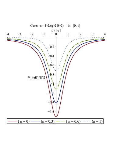
Figure 1: Effective potential for a massless test particle with , in the spacetime geometry (40) with . The ordinate is ; the abscissa is . -
ii)
If being , according to (66) we have three real critical points in this case, because . From (69) we have then are local maximum values of the potential, i.e. . On the other hand from (68) we have , implying is a local minimum value of the potential. By looking at the asymptotic behavior as , we can conclude is the global maximum value of the potential, whereas is the global minimum value. Now, using (67), for with and , we have,
(70) From the last relation we conclude that for this photon . because , and it always can pass above this effective potential. See Fig. 2.
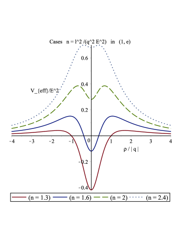
Figure 2: Effective potential for a massless test particle with , in the spacetime geometry (40) with . The ordinate is ; the abscissa is . -
iii)
Finally, if where , according to (68) we have this implies the potential has a local maximum located at . Moreover, since as we conclude that is the maximum value of the effective potential. Now, using (67), for , with , we obtain,
(71) The equation can only be satisfied for photons with , this corresponds to an unstable circular orbit. Whereas, photons with cannot pass through this effective potential because for them . See Fig. 3.
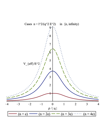
Figure 3: Effective potential for a massless test particle with , in the spacetime geometry (40) with . The ordinate is ; the abscissa is . 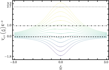
Figure 4: Effective potential curves for several values of , horizontal lines represent important values of the parameter .
Photon sphere: We have shown that in the spacetime geometry (40) is possible that some photons to follow circular orbits. Specifically, according to (71), a photon with feel a potential so that , which implies that this could follow a circular geodesic. This orbit is called the photon circle (for details seepho_orb ). Due to the spherical symmetry, the condition defines a collection of infinitely many such orbits, therefore the last photon orbit is also called photon sphere pho_orb . According to Wald , the impact parameter will be , and hence the capture cross-section for a light beam is , or in terms of the WH throat, , this becomes . The photon sphere can cast a wormhole shadow for an observer at infinity. This shadow is a disk specified by its radius and it gives an apparent size and shape of WH throat. For a static spherically symmetric asymptotically flat wormhole is just the impact parameter . So for example, for the Ellis WH which in terms of the Ellis WH throat , becomes , see EllisShadows for details. In our case for the WH geometry (40) we get which is bigger that of the Ellis WH.
Asymptotically behavior of the metric (40) at infinity: Expanding the metric in powers of around give us
| (72) |
This allow us to write the line element as,
| (73) |
which behaves asymptotically as the exterior region of the Reissner-Nordström black hole: , without Arnowitt-Deser-Misner (ADM) mass () and with imaginary charge (). The latter is a immediate consequence of the violation of the null and weak energy conditions in the region of weak field by the NLED Lagrangian density (38).
VII Conclusions
In this work, in the Einstein’s gravity context, we have constructed a new SSS-AF T-WH solution which can be interpreted as a non-trivial redshift modification of the Ellis WH. The sources are; a self-interacting phantom scalar field, which was introduced to satisfy the flare-out condition; and a nonlinear electrodynamics field which becomes the Maxwell theory in the limit of weak field. Moreover, this nonlinear electrodynamics satisfying the WEC in a limited region of the spacetime which contains the WH throat. We also study the source of the T-WH from the perspective of modified gravity, using a Gauss-Bonnet correction term, wich provide the necessary conditions for the existence of such solution without claiming the existence of a panthom field. Our T-WH metric is determined by only one parameter , which can be associated to the magnetic charged, and defines the WH throat as . Thus, in the limit of zero magnetic charge, the Minkowski metric is recovered. Moreover, we found that this solution has a WH shadow of radius which is bigger than the shadow radius of the Ellis WH.
To a better characterization of the wormhole we have just presented is necessary the study of their quasinormal modes, its corresponding Penrose diagram and its stability. This last behavior is essential in order to guarantee the traversability of this wormhole. We hope to return to these issues in a future work.
Appendix A Null and weak energy conditions in GR
For a energy-momentum tensor , the null energy condition (NEC), stipulates that for every null vector, , yields . Following WEC , for a diagonal energy-momentum tensor , which can be conveniently written as,
| (74) |
where may be interpreted as the rest energy density of the matter, whereas , and are respectively the pressures along the , and directions. In terms of (74) the NEC implies:
| (75) |
The weak energy condition (WEC) states that for any timelike vector , (i.e., ), the energy-momentum tensor obeys the inequality , which means that the local energy density as measured by any observer with timelike vector is a non-negative quantity. For an energy-momentum tensor of the form (74), the WEC will be satisfied if and only if,
| (76) |
-
•
NEC and WEC for a self-interacting scalar field
-
•
NEC and WEC for the nonlinear electrodynamics field ; pure-magnetic case
- •
Appendix B Domain of validity of the WEC and NEC for the NLED model
To find the region where the WEC and the NEC are valid, let’s notice the following:
| (90) |
then,
| (91) |
Whereas,
| (92) |
hence,
| (93) |
Thus, according to (82), (83) and given that for the pure-magnetic is positive defined (13), the NLED model holds the WEC (i.e. and ) only if,
| (94) |
However, since in the WH domain , or in terms of the electromagnetic invariant , then in the wormhole spacetime (40) the NLED holds the WEC only if,
| (95) |
Appendix C Field equations of GR-NLED-SF theory
In this appendix we include the more general form of the equations of motion for GR-NLED-SF theory that are satisfied by a SSS metric.
Since the spacetime is static and spherically symmetric, the more general form of the electromagnetic field tensor is given by,
| (96) |
Hence, for an arbitrary NLED Lagrangian density , the non-vanishing components of the NLED energy-momentum tensor, assuming the SSS metric (9) and the more general SSS electromagnetic field tensor (96), are given by,
| (97) | |||
| (98) |
Inserting the above components in the Einstein field equations , for the metric ansatz (9) and scalar field energy-momentum tensor (11), yield,
| (99) | |||
| (100) | |||
| (101) |
Bibliography
References
- (1) A. Einstein and N. Rosen, The Particle Problem in the General Theory of Relativity, Phys. Rev. 48, 73 (1935).
- (2) M. D. Kruskal, Maximal Extension of Schwarzschild Metric, Phys. Rev. 119, 1743 (1960); R. W. Fuller and J. A. Wheeler, Causality and Multiply Connected Space-Time Phys. Rev. 128, 919 (1962).
- (3) M. S. Morris, K. S. Thorne, Wormholes in Spacetime and their use for Interstellar Travel: A Tool for Teaching General Relativity, Am. J. Phys 56, 395 (1988).
- (4) M. S. Morris, K. S. Thorne, and U. Yurtsever, Wormholes, Time Machines, and the Weak Energy Condition, Phys. Rev. Lett 61, 1446 (1988).
- (5) G. W. Gibbons, D.A. Rasheed, Dyson pairs and zero mass black holes, Nucl. Phys. B 476, 515 (1996).
- (6) L. P. Chimento and R. Lazkoz, Constructing Phantom Cosmologies from Standard Scalar Field Universes, Phys.Rev.Lett. 91 (2003) 211301.
- (7) A. Paliathanasis and G. Leon, Dynamics of a two scalar field cosmological model with phantom terms, Class. Quantum Grav. 38 075013 (2021).
- (8) M. Cataldo, F. Arevalo, and P. Mella, Canonical and phantom scalar fields as an interaction of two perfect fluids, Astrophys.Space Sci. 344 (2013) 495-503.
- (9) S. Hannenstadt, Dark energy and dark matter from cosmological observations, Int. J. Mod. Phys. A 21, 1938 (2006)
- (10) J. Dunkle et al., Five-Year Wilkinson Microwave Anisotropy Probe (WMAP) Observations: Likelihoods and Parameters from the WMAP data Astrophys. J. Suppl. Ser. 180, 306 (2009)
- (11) R. R. Caldwell, M. Kamionkowski, and N. N. Weinberg, Phantom energy and cosmic doomsday, Phys. Rev. Lett. 91, 071301 (2003).
- (12) S. Dutta and R. J. Scherrer, Dark Energy from a Phantom Field Near a Local Potential Minimum, Phys. Lett. B 676, 12 (2009).
- (13) G. Alestas, L. Kazantzidis, and L. Perivolaropoulos, tension, phantom dark energy, and cosmological parameter degeneracies, Phys. Rev. D 101, 123516 (2020).
- (14) F. X. Linares Cedeño, N. Roy, and L. A. Ureña-López, Tracker phantom field and a cosmological constant: Dynamics of a composite dark energy model, Phys. Rev. D 104, 123502 (2021).
- (15) Ming-Hsun Li and Kwei-Chou Yang, Galactic Dark Matter in the Phantom Field, Phys. Rev. D 86, 123015.
- (16) K. A. Bronnikov and J. C. Fabris, Regular phantom black holes, Phys. Rev. Lett. 96, 251101 (2006).
- (17) L. Zhang, X. Zeng and Z. Li, AdS black hole with Phantom scalar field, Adv. High Energy Phys. 2017, 4940187 (2017).
- (18) H. G. Ellis, Ether flow through a drainhole: A particle model in general relativity, J. Math. Phys 14, 104 (1973); K. A. Bronnikov, Scalar-tensor theory and scalar charge, Acta Phys. Pol. B 4, 251 (1973).
- (19) K. K. Nandi, Y.-Z. Zhang, A. V. Zakharov, Gravitational lensing by wormholes, Phys. Rev. D. 74, 024020 (2006); F. Abe, Gravitational microlensing by the Ellis wormhole, Astrophys. J. 725, 787 (2010); K. Nakajima and H. Asada, Deflection angle of light in an Ellis wormhole geometry, Phys. Rev. D 85, 107501 (2012); N. Tsukamoto, Strong deflection limit analysis and gravitational lensing of an Ellis wormhole, Phys. Rev. D 94, 124001 (2016); B. Amrita and A. A. Potapov, On strong field deflection angle by the massless Ellis-Bronnikov wormhole, Mod. Phys. Lett. A 34, 1950040 (2019).
- (20) J. L. Blázquez Salcedo, X. Y. Chew, and J. Kunz, Scalar and axial quasinormal modes of massive static phantom wormholes, Phys. Rev. D. 98, 044035 (2018).
- (21) T. Ohgami and N. Sakai, Wormhole shadows, Phys. Rev. D. 91, 124020 (2015).
- (22) C. Armendariz-Picon, On a class of stable, traversable Lorentzian wormholes in classical general relativity, Phys, Rev. D. 65, 104010 (2002); H. Shinkai and S. A. Hayward, Fate of the first traversible wormhole: black-hole collapse or inflationary expansion, Phys. Rev. D 66, 044005 (2002); J. A. Gonzalez, F. S. Guzman, and O. Sarbach, Instability of wormholes supported by a ghost scalar field. II. Nonlinear evolution, Class. Quantum Grav. 26, 015011 (2009); A. Doroshkevich, J. Hansen, I. Novikov, and A. Shatskiy, Passage of radiation through wormholes, Int. J. Mod. Phys. D 18, 1665 (2009); K. A. Bronnikov, J. C. Fabris, and A. Zhidenko, On the stability of scalar-vacuum space-times, EuroPhys J. C 71, 1791 (2011); K. K. Nandi et al., Stability and instability of Ellis and phantom wormholes: Are there ghosts?, Phys. Rev. D 93, 104044 (2016); F. Cremona, F. Pirotta, and L. Pizzocchero, On the linear instability of the Ellis-Bronnikov-Morris-Thorne wormhole, Gen. Relativ. Grav. 51, 19 (2019).
- (23) A. A. Shatskii, I. D. Novikov, and N. S. Kardashev, A dynamic model of the wormhole and the Multiverse model, Physics-Uspekhi 51, 457 (2008); K. A. Bronnikov, L. N. Lipatova, I. D. Novikov, and A. A. Shatskiy, Example of a stable wormhole in general relativity, Grav. Cosmo. 19, 269 (2013).
- (24) M. Born, L. Infeld: Foundations of the New Field Theory, Proc. Roy. Soc. A144 (1934) 425–451.
- (25) H. Euler and B. Kockel, The scattering of light by light in the Dirac theory, Naturwiss. 23, 246 (1935).
- (26) W. Heisenberg and H. Euler, Folgerungen aus der Diracschen Theorie des Positrons. Z. Phys 98 (11-12), 714–732 (1936); English translation: Consequences of Dirac’s Theory of Positrons, arXiv: physics/0605038.
- (27) E. Ayón-Beato and A. García, Regular Black Hole in General Relativity Coupled to Nonlinear Electrodynamics, Phys. Rev. Lett. 80, 5056 (1998); Non-Singular Charged Black Hole Solution for Non-Linear Source, Gen. Rel. Gravit., 31, 629 (1999); New Regular Black Hole Solution from Nonlinear Electrodynamics, Phys. Lett., B 464, 25 (1999); The Bardeen Model as a Nonlinear Magnetic Monopole, Phys. Lett. B 493, 149 (2000); Four Parametric Regular Black Hole Solution, Gen. Rel. Grav. 37, 635 (2005).
- (28) A. V. B. Arellano, N. Bretón and R. Garcia-Salcedo, Some properties of evolving wormhole geometries within nonlinear electrodynamics, Gen. Relativ. Gravit. 41 (2009) 2561.
- (29) K. A. Bronnikov, Nonlinear electrodynamics, regular black holes and wormholes, Int. J. Mod. Phys. D 27, 1841005 (2018).
- (30) H. Yajima and T. Tamaki, Black hole solutions in Euler-Heisenberg theory, Phys. Rev. D 63 064007 (2001); M. Guerrero, D. Rubiera-Garcia. Nonsingular black holes in nonlinear gravity coupled to Euler-Heisenberg electrodynamics. Physics Letters B 788, 446-452 (2019).
- (31) M. Novello, S. E. Perez Bergliaffa, and J. M. Salim, Singularities in General Relativity coupled to nonlinear electrodynamics, Class. Quant. Grav. 17 (2000) 3821-3832.
- (32) K. A. Bronnikov, R. K. Walia, Field sources for Simpson-Visser space-times, arXiv: 2112.13198.
- (33) A. V. B. Arellano and F. S. N. Lobo, Non-existence of static, spherically symmetric and stationary, axisymmetric traversable wormholes coupled to nonlinear electrodynamics, Class. Quantum Grav. 23 7229 (2006).
- (34) P. Cañate, N. Breton, Black Hole-Wormhole transition in (2+1) Einstein -anti- de Sitter Gravity Coupled to Nonlinear Electrodynamics, Phys. Rev. D 98 104012 (2018).
- (35) P. Cañate, N. Breton, L. Ortiz, -dimensional Static Cyclic Symmetric Traversable Wormhole: Quasinormal Modes and Causality, Class. Quant. Grav. 37 055007 (2020).
- (36) P. Cañate, D. Magos, N. Breton, Nonlinear electrodynamics generalization of the rotating BTZ black hole, Phys. Rev. D 101 064010 (2020).
- (37) E. Ramirez, D. J. Schwarz, inflation is not excluded, Phys. Rev. D 80 023525 (2009).
- (38) V. N. Senoguz, Q. Shafi, Chaotic inflation, radiative corrections and precision cosmology, Phys. Lett. B 668: 6 (2008).
- (39) D. J. Amit, E. Rabinovici, Breaking of Scale Invariance in Theory: Tricriticality and Critical End Points, Nucl. Phys. B 257 371-382 (1985).
- (40) I. Takyi, M. K. Matfunjwa, H. Weigel, Quantum corrections to solitons in the model, Phys. Rev. D 102, 116004 (2020).
- (41) S A Fulling, Alternative vacuum states in static space-times with horizons, J. Phys. A: Math. Gen. 10 917 (1977).
- (42) S. A. Fulling, F. J. Narcowich and R. M. Wald, Singularity structure of the two-point function in quantum field theory in curved spacetime, II. Ann. Physics 136, 243-272 (1981).
- (43) D. N. Page, Thermal stress tensors in static Einstein spaces, Phys. Rev. D 25, 1499 (1982).
- (44) W. Rindler, Relativity-Special, General and Cosmology (Oxford University Press, New York, 2001).
- (45) M. Visser, Lorentzian Wormholes: from Einstein to Hawking, AIP Press, New York, 1995; H. Stephani, D. Kramer, M. MacCallum, C. Honselaers, and E. Herlt, Exact solutions to Einstein’s Field Equations, Second Edition, Cambridge University Press, Cambridge, U.K., 2003.
- (46) C. R. Cramer, Using the Uncharged Kerr Black Hole as a Gravitational Mirror, General Relativity and Gravitation. 29, 445–454 (1997); C. M. Claudel, K. S. Virbhadra, and G. F. R. Ellis, The Geometry of Photon Surfaces, J. Math. Phys. 42, (2001); T. Edward, Spherical Photon Orbits Around a Kerr Black Hole, General Relativity and Gravitation 35, 1909–1926 (2003); P. V. P. Cunha, C. A. R. Herdeiro, and E. Radu, Fundamental photon orbits: black hole shadows and spacetime instabilities, Phys. Rev. D 96, 024039 (2017).
- (47) R. M. Wald, General Relativity, University of Chicago Press (1984).
- (48) G. Antoniou, A. Bakopoulos, P. Kanti, B. Kleihaus, and J. Kunz, Novel Wormhole Solutions in Einstein-Scalar-Gauss-Bonnet Theories, arXiv:1904.13091 (2019)
- (49) P. Kanti, B. Kleihaus, and J. Kunz, Wormholes in Dilatonic Einstein-Gauss-Bonnet Theory, Phys. Rev. Lett. 107, 271101 (2011)
- (50) P. Kanti, N. E. Mavromatos, J. Rizos, K. Tamvakis, and E. Winstanley, Dilatonic Black Holes in Higher Curvature String Gravity, Phys. Rev. D 54, 5049 (1996)
- (51) P. Cañate, J. Sultana, D. Kazanas, Ellis wormhole without a phantom scalar field, Phys. Rev. D 100, (2019) 064007
- (52) P. Cañate, N. Breton, New exact traversable wormhole solution to the Einstein-scalar-Gauss-Bonnet equations coupled to power-Maxwell electrodynamics, Phys. Rev. D 100, (2019) 064067
- (53) S. Nojiri, S.D. Odintsov, M. Sasaki, Gauss-Bonnet dark energy, Phys. Rev. D 71, 123509 (2005); M. Heydari-Fard, H. Razmi, M. Yousefi, Scalar-Gauss-Bonnet gravity and cosmic acceleration: Comparison with quintessence dark energy, Int. J. Mod. Phys. D 26 1750008 (2017); Koivisto, Tomi and Mota, David F., Cosmology and Astrophysical Constraints of Gauss-Bonnet Dark Energy, Phys. Lett. B, 644, 104-108, (2007); T. Kolvisto, D. Mota, Gauss-Bonnet quintessence: Background evolution, large scale structure, and cosmological constraints, Phys. Rev. D 75, 023518 (2007).
- (54) Tsujikawa, Shinji and Sami, M., String-inspired cosmology: Late time transition from scaling matter era to dark energy universe caused by a Gauss-Bonnet coupling, JCAP 01, 006 (2007).
- (55) Nojiri, Shin’ichi and Odintsov, Sergei D. and Sami, M., Dark energy cosmology from higher-order, string-inspired gravity and its reconstruction, Phys. Rev. D, 74, 046004, (2006); Cognola, Guido and Elizalde, Emilio and Nojiri, Shin’ichi and Odintsov, Sergei and Zerbini, Sergio, String-inspired Gauss-Bonnet gravity reconstructed from the universe expansion history and yielding the transition from matter dominance to dark energy, Phys. Rev. D, 75, 086002, (2007).
- (56) Odintsov, S.D. and Oikonomou, V.K. and Fronimos, F.P., Non-Minimally Coupled Einstein Gauss Bonnet Inflation Phenomenology in View of GW170817, Annals Phys. 420, 168250, (2020).
- (57) G. Antoniou, A. Bakopoulos, P. Kanti, Black hole solutions with scalar hair in the Einstein-scalar-Gauss-Bonnet theories, Phys. Rev. D 97, 084037 (2018); A. Bakopoulos, G. Antoniou, P. Kanti, Novel Black-Hole Solutions in Einstein-Scalar-Gauss-Bonnet Theories with a Cosmological Constant, Phys. Rev. D 99, 064003 (2019).