NT@UW-09-18
Electromagnetic Form Factors and
Charge Densities From Hadrons to Nuclei
Abstract
A simple exact covariant model in which a scalar particle is modeled as a bound state of two different particles is used to elucidate relativistic aspects of electromagnetic form factors . The model form factor is computed using an exact covariant calculation of the lowest-order triangle diagram. The light-front technique of integrating over the minus-component of the virtual momentum gives the same result and is the same as the one obtained originally by Gunion et al. by using time-ordered perturbation theory in the infinite-momentum-frame. The meaning of the transverse density is explained by providing a general derivation, using three spatial-coordinates, of its relationship with the form factor. This allows us to identify a mean-square transverse size . The quantity is a true measure of hadronic size because of its direct relationship with the transverse density. We show that the rest-frame charge distribution is generally not observable by studying the explicit failure to uphold current conservation. Neutral systems of two charged constituents are shown to obey the conventional lore that the heavier one is generally closer to the transverse origin than the lighter one. It is argued that the negative central charge density of the neutron arises, in pion-cloud models, from pions of high longitudinal momentum that reside at the center. The non-relativistic limit is defined precisely, and the ratio of the binding energy to the mass of the lightest constituent is shown to govern the influence of relativistic effects. We show that the exact relativistic formula for is the same as the familiar one of the three-dimensional Fourier transform of a square of a wave function for very small values of , but this only occurs values of less than about 0.001. For masses that mimic the quark-di-quark model of the nucleon we find that there are substantial relativistic corrections to the form factor for any value of . A schematic model of the lowest -states of nuclei is developed. Relativistic effects are found to decrease the form factor for light nuclei but to increase the form factor for heavy nuclei. Furthermore, these lowest -states are likely to be strongly influenced by relativistic effects that are order 15-20%.
pacs:
11.80.-m, 12.39.Ki,13.40.Gp,25.30.BfI Introduction
The text-book interpretation of nucleon electromagnetic form factors is that their three-dimensional Fourier transforms are measurements of the charge and magnetization densities. This interpretation is deeply buried in our thinking and continues to guide intuition as it has since the days of the Nobel prize-winning work of HofstadterHofstadter:1956qs . Nevertheless, the relativistic motion of the constituents of the system causes the text-book interpretation to be incorrect.
The preceding statement leads to a number of questions, the first being: Is the statement correct? If correct, how relativistic does the motion of the constituents have to be? Why is it that the relativistic motion of the constituents and not that of the entire system that causes the non-relativistic approach to fail? It is probably true that the answers to these questions are displayed within the existing literature. However, obtaining general clear answers has been sufficiently difficult that posing even the first question of this paragraph would not lead to a unanimous answer by all professionals in the field.
This paper offers the strategy of using a simple model, a generalization of the model used by Weinberg Weinberg:1966jm to illustrate advantages of using the infinite momentum by choosing frame that was used by Gunion et al. Gunion:1973ex to explore form factors and hadronic interactions at high-momentum transfer. We take the interaction Lagrangian density to be of the form in which all of the fields are bosons.The particle of mass represents the bound state of the two different constituents of masses respectively. Thus the represents the hadron or nucleus with the representing the quark or nucleonic constituents. Mass renormalization effects are ignored. We can choose either or both of the constituents to be charged and thus discuss charged and neutral particles.
The motivation to pose questions regarding the meaning of electromagnetic form factors at this point in time arises from recent experimental work, especially the discovery that the ratio of the proton’s electric to magnetic Sachs form factors drops rapidly (please see the reviews reviews ) and from our recent finding Miller:2007uy , based on measurements and the use of the transverse density that the charge density at the neutron’s center is negative. The nucleon transverse density , the two-dimensional Fourier transform of is the infinite momentum frame charge densitynotation located at a transverse separation from the center of transverse momentumsoper1 ; mbimpact ; diehl2 ; Carlson:2008zc . This quantity has a direct relationship to matrix element of a density operator. The usual three-dimensional Fourier transforms of and do not because the initial- and final-state nucleons have different momentum, and therefore different wave functions. This is because the relativistic boost operator that transforms a nucleon at rest into a moving one changes the wave function in a manner that depends on the momentum of the nucleon. However, we expect that there are non-relativistic conditions for which the text-book interpretation is correct. We aim to explore those conditions by choosing appropriate values of the masses .
Here is the outline we follow. The form factor for the situation in which the and carry a single unit of charge, but the is neutral, is computed using an exact covariant calculation of the lowest-order triangle diagram in Sect. II. This is followed by a another derivation using the light-front technique of integrating over the minus-component of the virtual momentum in Sect. III that obtains the same form factor. This is also the result obtained originally by Gunion:1973ex by using time-ordered perturbation theory in the infinite-momentum-frame IMF. Thus three different approaches yield the same exact result for this model problem. Any approximation that does not yield the same form factor is simply not correct. The asymptotic limit of very high momentum transfer is also studied. The next section (IV) explains the transverse density of the model, its central value, a general derivation of its relationship with the form factor using three dimensional spatial coordinates and the meaning of hadronic radii. Section V displays the spatial wave function in terms of three spatial coordinates. Section VI shows that the rest-frame charge distribution is generally not observable. Section VII is concerned with the question of whether neutral systems of two constituents obey the conventional lore that the heavier one is generally closer to the origin than the lighter one. The non-relativistic limit is defined and applied to a variety of examples in Section VIII. The exact formula for the form factor morphs into the familiar one of the three-dimensional Fourier transform for sufficiently large values of the constituent mass divided by the binding energy of the system. Examples that are motivated by the pion, deuterium, nucleon and heavy nuclei are provided. This work is summarized in Section IX.
II Exact form factors using a simple model
The model Lagrangian density is given by where and represent three scalar fields of masses and respectively and is a coupling constant. One can take two or three of these fields to carry charge to make up a system of definite charge (including the case when the hadron is neutral). The effects of mass renormalization are not considered here because we aim to use a simple model to provide easily calculable examples and illustrate specific points. The condition is used to insure that the hadron is stable.
We start with the situation in which the each carry a single positive charge and is neutral. The form factor for a space-like incident photon of four-momentum , incident on a target of four-momentum interacting with the of mass is given, to lowest order in , by the single Feynman diagram of Fig. 1. We take the model electromagnetic current (in units of the proton charge) as given by
| (1) |
and find
| (3) | |||||
Proceed by combining the denominators using the Feynman procedure and shifting the origin of the convergent integral to find
| (4) |
where Use
| (5) |
to find
| (6) |
The integral over can be done in closed form with the result
| (7) |
The above expression shows that current conservation is satisfied and that the form factor can be obtained from any component of the current operator . The final result for the form factor is
| (8) |
This closed form expression is the key result of this paper. It can be modified to describe a variety of different physical situations.
III Infinite momentum frame/Light Front Representation
We derive the light front representation by starting with the form factor of Eq. (3) and integrating over . This procedure is simplified by choosing , so that notation and evaluating the component of the electromagnetic current operator. In the present Section the convention is that for the four-vector . Then Eq. (3) becomes
| (9) | |||
| (10) |
If we integrate over the upper half of the complex plane we find a non-zero contribution only for the case . Carrying out the integral leads to
| (11) |
Next change variables by defining
| (12) |
so that
| (13) |
Further define the relative transverse momentum
| (14) |
so that the form factor can be re-expressed as
| (15) |
This is the expression obtained in Ref. Gunion:1973ex , by using time-order-perturbation theory in the infinite momentum frame. Integration over leads to the same result for this example.
It is useful to re-express the result Eq. (15) in terms of a wave function with
| (16) |
In that case
| (17) |
as found in Ref. Gunion:1973ex .
The integration over is convergent so we carry out the integration over by combining the propagators and shifting the origin. This gives
| (18) |
The integral over can be done with the result that
| (19) |
This is the same as our previous exactly computed result, Eq. (8). Thus evaluation in the infinite momentum frame or the equivalent (for this model) light front technique of integration over yields the exact result.
III.1 Asymptotic Behavior of the Form Factor
The limit of very high is of considerable interest. One wants to see how the quark counting rules emerge from an exact calculation, even if the model is very simple. To this end we note, that the integral Eq. (19) can be evaluated exactly in the limit that with . Then measuring in units of () we find
| (20) |
so that
| (21) |
Thus the leading asymptotic behavior is
| (22) |
Thus the power-law fall-off expected from the quark-counting rules appears, but it is modified by the presence of the logarithms. This behavior is not associated with taking to zero because in all cases we have as required for the particle to be stable. Thus the asymptotic behavior () associated with Eq. (22) is expected to be universal for this model. Note however, from Eq. (21) that the approach to this asymptotic form is very slow.
IV Electromagnetic form factors measure transverse densities and transverse radii
The expression Eq. (17) is noteworthy because the form factor is expressed as a three-dimensional integration that involves momentum-space wave functions evaluated at different initial and final momenta. If the factor multiplying were replaced by a constant Eq. (17) would be similar to the usual expression for the form factor. We clarify this comparison by expressing the wave function of Eq. (16) and Eq. (17) in transverse position space, with canonically conjugate to the transverse momentum variable :
| (23) | |||
| (24) |
with the phase space factor incorporated in the wave function. Then the form factor Eq. (17) can be re-expressed as
| (25) |
Further simplify by replacing the relative transverse position variable by the transverse position variable of the charged parton . We have
| (26) | |||
| (27) | |||
| (28) |
where the middle equation sets the transverse center of momentum to zero. Use Eq. (28) in Eq. (25) to find
| (29) |
which can be re-written as
| (30) |
with the transverse density given by
| (31) |
The transverse density has been derived previously mbimpact ; diehl2 as the integral of the impact parameter generalized parton distributions GPD over all values of . The quantity gives the probability that a quark of longitudinal momentum fraction resides at a transverse position mbimpact ; diehl2 . For the present model
| (32) |
The transverse density is also the integral of the three-dimensional infinite momentum frame density over all values of the longitudinal position coordinate miller:2009qu .
The transverse density is directly obtainable from experiment via the inverse Fourier transform of Eq. (30) provided the electromagnetic form factor is measured for sufficiently large values of . The momentum transfer is transverse in direction so that information about the longitudinal position or momentum is not available. There is no way to use only measured values of to determine .
IV.1 Singular central density
Before proceeding it is worthwhile to point out that the model central density is singular. This arises as a consequence of the zero range nature of the coupling. The transverse density is an integral involving the singular function which varies as for . The question of the singularity of the central transverse density is interesting to the present author because of recent work miller:2009qu showing that for the pion is likely to approach infinity as approaches zero. We may study the limit as approaches 0 by using the asymptotic limit of the form factor Eq. (22). The density for near zero is controlled by the form factor at large values of . We use the inverse of Eq. (29) to write
| (33) |
where is a momentum transfer large enough so that so that Eq. (22) is valid, and is a fixed positive number small enough so that to any desired precision. Changing variables to shows that
| (34) |
which is the central singular charge density arising from the behavior of the asymptotic form factor.
IV.2 Transverse Charge Density from a more general perspective
For a spin-0 system, the form factor , Eq. (3) may be computed, in the Drell-Yan DY frame , by using
| (35) |
The spatial structure of a nucleon can be examined if one uses soper1 ; mbimpact ; diehl2 . The state with transverse center of mass set to 0 is formed by taking a linear superposition of states of transverse momentum:
| (36) |
where are plane wave states and is a normalization factor satisfying . The normalization of the states is given by
| (37) |
References mb1 ; diehl use wave packet treatments that avoid states normalized to functions, but this leads to the same results as using Eq. (36). Note however, the relevant range of integration in Eq. (36) must be restricted to to maintain the interpretation of a nucleon moving with well-defined longitudinal momentummb1 . Thus we use a frame with very large . It is in just such a frame that the interpretation of a nucleon as a set of a large number of partons is valid.
We evaluate the density operator in the infinite momentum frame in which the spatial coordinates are , and time is . We therefore do not write the dependence in any function below. The infinite momentum frame charge density operator (in units of the proton charge) is given by
| (38) |
and the density itself by
| (39) |
IV.3 Mean-squared transverse radii and mean-squared effective radii
The two-dimensional Fourier transform of Eq. (30) may be expanded as a power series in as
| (41) |
where the mean-squared transverse radius is given in terms of the transverse density as
| (42) |
and a direct relation with the transverse density is evident. In contrast, the usual procedure is to write
| (43) |
where we denote the effective mean-squared radiusMiller:2007kt . The quantity has no direct relationship with a density unless the system is non-relativistic. Thus we maintain that is the basic quantity related to an underlying density. However, once the effective mean-squared radius is determined, the fundamental is known immediately because a comparison of Eq. (41) and Eq. (43) reveals that
| (44) |
V Wave function as a function of three position variables
The previous section shows that the form factor is simply related to the three-dimensional coordinate-space density that depends on in the infinite momentum frame. Given the simplicity of our model, we should be able to identify a wave function and density.
The basic idea is that the position variable of a particle is canonically conjugate to the plus-component of the momentum. The momentum of the charged constituent is , and its canonical longitudinal position variable is with Pirner:2009zz . The canonical longitudinal position variable for the other particle can be taken as . So we can convert the wave function of Eq. (24) to one expressed entirely in coordinate space. We find
| (45) |
which preserves the normalization condition that . Note that is a relative variable and that is the variable for the position of the charged constituent. This wave function displays no spherical symmetry–the longitudinal and transverse position dependence are not related. Another point is that the wave function Eq. (45) explicitly depends on the momentum . As approaches infinity, the value of must be very small to prevent from being very large and causing the integral on Eq. (45) to vanish. This means that the system can be thought of as having a pancake or disc shape. For this reason, the position really does correspond to the center of the hadron. We shall show below, that in the non-relativistic limit, rotational symmetry emerges.
The wave function can be computed in closed form for the special case . Using Eq. (24) in Eq. (45) with the stated parameters leads to the result
| (46) | |||
| (47) |
For this simple example, the and dependence factorizes, showing the explicit violation of rotational symmetry. The formula Eq. (47) shows also how the spatial extent contracts with the increase in value . We note that it is not useful to use the spatial wave function to compute the form factor because of the appearance of the factor in the exponential of Eq. (25).
VI The Rest Frame Charge Distribution is Generally Not Observable
The concept of a charge density that depends on three spatial variables, but not on the time, is inherently non-relativistic. This is because the use of only three variables involves replacing a four-dimensional quantity by one involving only three dimensions. One procedure, discussed above in Sect. II, is to evaluate the Feynman diagram of Fig. 1 by integrating over the component of the virtual momentum . This leads to a formalism in which the form factor depends on a Fourier transform of the square of a wave function that depends both on position and momentum variables.
One can try to recover the more familiar three-spatial dimension formalism by evaluating the Feynman diagram of Fig. 1 using the time-ordered-perturbation theory TOPT formalism in the rest frame. One proceeds by integrating over all times, with the exponential oscillating factors converted into energy denominators. In the TOPT formalism any given Feynman diagram is the sum of several TOPT diagrams. In the present case, the sum of the two TOPT diagrams of Fig. 2 leads to the Feynman diagram of Fig. 1. Only Fig. 2a corresponds to measuring a density. The term of Fig. 2b corresponds to the hadronic part of the incident photon wave function interacting with the target.
One can examine the contribution of the term of Fig. 2a, . It is given Gunion:1973ex by
| (48) |
an expression that leads to the correct result in the infinite momentum frame () Gunion:1973ex . This expression can be interpreted as involving an initial and a final state wave function if one interprets the energy denominators (multiplied by phase space factors) as wave function expressed in momentum space. The symbol used above refers to the approximation of keeping only a single TOPT diagram. For simplicity we take the example, and also work in the target rest frame: to isolate the rest frame charge distribution. Then . The four vector . There are three integrals appearing on the right-hand-side of Eq. (48):
| (49) | |||
| (50) | |||
| (51) |
Thus we arrive at the four-vector equality
| (52) |
Maintaining current conservation requires that the matrix element of vanishes. Taking the scalar product of Eq. (52) with leads to the requirement:
| (53) |
where . The right-hand-side of Eq. (53) is defined as so that comparing to unity provides a reasonable measure of the failure of this approximation to uphold current conservation. We express all momenta and mass in units of the target mass (=1), take as an examples and 0.6 and plot the numerical results in Fig. 3. Both and are measured in units of the target mass , taken as unity. Thus the natural scale of any quantity is unity. We see that current conservation is massively violated in the rest frame for systems in which is not very small. In that case, the expression that potentially depends on the square of the wave function or density has no independent physical reality.
VII Neutral Systems
Previous work Miller:2007uy showed that the central transverse density of the neutron is negative. This contrasts with the long held view that there must be positive charge density at the center to neutralize the effects of a negatively charged pionic cloud that occupies the exterior. This result demands interpretation Miller:2008jc -Rinehimer:2009sz .
One relevant question is whether or not the intuition that a neutral system consisting of a heavy charge positively charged particle and a negatively charged lighter particle disobeys the standard intuition that the averaged squared charged radius is negative, when the charge density is evaluated in the infinite momentum frame. We examine this question in our model by taking the (of mass ) to be positively charged and the (of mass to be negatively charged.
The form factor of this model can be obtained by using Eq. (8) by including a second term obtained by interchanging and and putting a minus sign in front. That operation gives the result
| (54) |
The results of a numerical evaluation using and are shown in Fig. 4. One observes the rise of from zero, which is the effect expected from non-relativistic, rest-frame considerations. The effective squared radius, defined in Eq. (43) is indeed negative. This is the same as expected from the intuition that the negatively charged light particle resides on the outside edge of the system.
One obtains the analytic result for the charge radius by taking the limit of very low in the expression for the form factor Eq. (54). The expression is simplified if one uses the (relevant for nucleon)assum case of . Then one finds:
| (55) |
A very accurate approximation (better than 1% for ) is
| (56) |
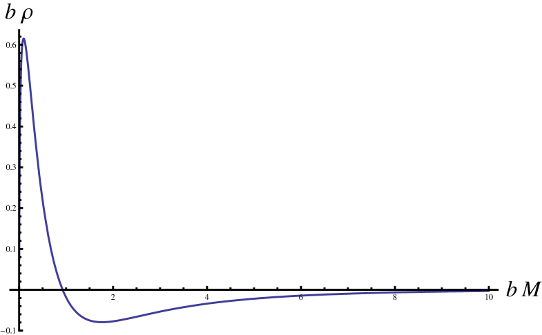
The radius is dominated by a singular term proportional to . Thus as expected the lighter constituent drifts to the edge of the nucleon. The conventional expectation is borne out on the light front. This is shown in more detail by plotting , as shown in Fig. 5. The positive charge density is concentrated at the center and the negative at the edge. This finding does not contradict the explanations offered in Refs. Miller:2008jc -Rinehimer:2009sz . Ref.Miller:2008jc argues that negative charge at high corresponds to negative charge at small values of . The model of Ref. Rinehimer:2009sz shows that one must include the finite size of the nucleon to obtain a computed that looks like the measured function. Thus the point-like nature of the constituents used here is unsurprisingly not relatistic. Moreover, in that model negatively charged pions reside both at the edge and at the center of the nucleon. The implication of Miller:2008jc is that the pions may have large values of longitudinal momentum fraction. This expectation is borne out by the model calculation Strikman:2009bd . Thus in pion cloud models of the nucleon pions that have a large longitudinal momentum tend to reside near the center of the nucleon.
VIII Non-relativistic Limit
The conventional lore is that the electromagnetic form factor is the Fourier transform of the charge density. In this section we see how this idea emerges by taking the non-relativistic limit.
Our starting point is the wave function Eq. (16) and the form factor Eq. (17). Recall that the quantity . We work in the rest frame and take the non-relativistic limit in which the energy , and , where is the third-component of the relative longitudinal momentum. Then Brodsky:1989pv ; Frankfurt:1981mk
| (57) |
where in conformation with non-relativistic notation, we define the positive binding energy so that
| (58) |
To obtain the non-relativistic expression we express the denominator appearing in Eq. (16) in terms of . This gives
| (59) | |||
| (60) | |||
| (61) | |||
| (62) | |||
| (63) |
where
| (64) |
In going from Eq. (59) to Eq. (63) we have ignored terms in of order three and higher. The result is that Eq. (63) is recognizable as times the inverse of the non-relativistic propagator.
The next step is to determine the coordinate form of the non-relativistic wave function (where is canonically conjugate to ) and to show that the non-relativistic form factor is a three-dimensional Fourier transform of . First use the non-relativistic approximation Eq. (63) in Eq. (16) to find
| (65) |
The coordinate-space wave function is given by
| (66) |
The expression Eq. (66) is seen as the standard result obtained for the bound state of a two-particle system interacting via an attractive delta function potential.
The wave functions Eq. (65) and Eq. (66) enable us to examine the condition needed for the approximations Eq. (57) to be valid. For Eq. (57) to work we need , but from the wave functions so that we require
| (67) |
for the non-relativistic approximation to be valid. More specifically let be the lighter of , then we may write the approximate condition as
| (68) |
The non-relativistic form factor is obtained by using Eq. (65) in the expression for the form factor Eq. (17), and taking the non-relativistic limit defined by the expressions:
| (69) | |||
| (70) | |||
| (71) |
The result is
| (72) |
This is the usual expectation that the form factor is a three-dimensional Fourier transform of the wave function. We may evaluate the integral immediately to find
| (73) |
where and the coupling constants and other constants enter in such a manner as to make .
In the remainder of this section we study the accuracy of the non-relativistic approximation by comparing the results of using Eq. (73) with the model-exact results of using Eq. (8) for several examples.
VIII.1 Bound state of two equal mass particles
With equal masses the bound state can be thought of as a toy meson or a deuteron. Use in Eq. (65) leads to the non-relativistic wave function with
| (74) |
with
| (75) |
The coordinate space wave function is then
| (76) |
Thus the wave function is the usual bound state wave function one obtains with a delta function binding interaction. We obtain the non-relativistic version of the form factor by using in Eq. (73) to find
| (77) |
where and the coupling constants and other constants enter in such a manner as to make .
We study the non-relativistic approximation numerically by comparing the exact model results Eq. (17) with those of the non-relativistic approximation Eq. (77). See Fig. 6. The figure shows two sets of results. In the upper panel the binding energy . This corresponds roughly to deuteron kinematics, in which the binding energy is of the order of a 0.004 of the deuteron mass. We see that the non-relativistic approximation is not accurate for values of greater than about 1. If one increases the binding energy to 0.1 , one sees that the non-relativistic approximation is not accurate for any value of . If one approximates a nucleon by taking 1 GeV, then GeV, which is much larger than a constituent quark mass. Thus the range of masses for which the non-relativistic approximation is valid is very narrow indeed.
We can gain some insight into the nature of the relativistic corrections to the charge radius by studying the low limit of the form factor of Eq. (8). One finds
| (78) |
where we use the notation to denote an effective radius squared that is not generally associated with the expectation of the square of a radius operator weighted by a density. The explicit evaluation gives
| (79) |
and
| (80) |
The non-relativistic limit corresponds to the limit of small values of , which corresponds to a small value of . So we expand the previous result to order to find
| (81) |
The non-relativistic value of the mean square radius, (which is a true mean square radius) is obtained by expanding the form factor for small values of :
| (82) |
which corresponds to the leading term of Eq. (81) in the limit that approaches 0. Comparing Eq. (81) with Eq. (82) shows that the former contains a series of terms that represent the boost corrections to the non-relativistic result. Each correction is positive and can be substantial. The figure 7 shows the ratio of the exact of the mean square radius to the non-relativistic approximation as a function of . We see that the non-relativistic approximation works well only for very small values of . Indeed, the ratio of the leading correction to the non-relativistic result is given by
| (83) |
For this ratio to be less than 10 %, must be less than one part in a thousand! Thus, within the framework of our toy model, the relativistic corrections can generally expected to be very substantial.
VIII.2 Quark-diquark model of the nucleon
Another interesting example is motivated by recent quark-diquark models of the nucleon Oettel:2000jj ; Horikawa:2005dh ; Cloet:2008re . We take . Then from Eq. (58) we have . In these, models current quarks acquire a large constituent mass due to the effects of dynamical chiral symmetry breaking. Therefore we take MeV, and MeV which corresponds via Eq. (58) to MeV and = 0.276. The non-relativistic expression for the form factor, for this case is obtain using the appropriate reduced mass as
| (84) | |||
| (85) |
Results comparing the exact form factor computed from Eq. (8) with that of Eq. (84) are shown in Fig. 8. The non-relativistic version gives a poor approximation to the exact form factor for all values of . This can be understood by considering the effective squared radius for this case. We find
| (86) |
The right-hand-side is evaluated as 0.887 for the present case, so that there is a substantial relativistic correction to the quantity for any non-zero value of . This means that one can not take a three-dimensional Fourier transform of the form factor to get a charge density even if the constituent masses are large.
VIII.3 Nuclear Physics and
We consider masses that correspond to electron scattering from a charged nucleon of mass (which is the free nucleon mass minus the average binding energy per nucleon of 8 MeV) bound in a nucleus of mass , with a spectator system of mass , where is the orbital separation energy. We measure all momenta in terms of MeV, and take the separation energy or about 46 MeV. The results for and are shown in Figs. 9 and 10
The startling finding is that the relativistic effects reduce the form factor for light nuclei, but increase it for heavy nuclei. Furthermore, the relativistic effects are larger for heavy nuclei than for light nuclei (for a fixed value of .)
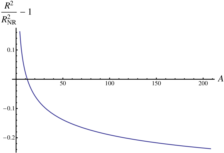
We obtain some analytic understanding by expanding the effective squared radius (defined in Eq. (78) in powers of . We find
| (87) |
We see that the first term is indeed the non-relativistic result, and that the second term changes sign for the value of that satisfies the equation or . This displayed in Fig. 11. It is also seen that the relativity causes very significant effects on the effective radii. Except for values of near 12, the changes are of the order of 10-15%. I expect that the specific values shown in Fig. 11 are highly model-dependent. Covariant models other than the model used here probably have have effects of different sizes. However, the large effects shown here cause one to wonder if relativity really may cause the true nuclear radii extracted from elastic electron scattering to differ by 10-20% from those appearing in tables. As noted above, we can expect that the model employed here is a reasonable representation of the lowest -state of heavy nuclei for which the range of the binding interactions is much less than the size of the system as a whole. For such states, the results of Fig. 11 should be a reasonably accurate guide, so that significant effects of relativity should be expected.
.
IX Summary
A relativistic model of a scalar particle is a bound state of two scalar particles and is used to elucidate relativistic aspects of electromagnetic form factors. First, the form factor for the situation in which the and carry a single unit of charge, but the is neutral is computed using an exact covariant calculation of the lowest-order triangle diagram. This is followed by a another derivation using the light-front technique of integrating over the minus-component of the virtual momentum in Sect. III that obtains the same form factor. This is also the result obtained originally by Gunion:1973ex by using time-ordered perturbation theory in the infinite-momentum-frame IMF. Thus three different approaches yield the same exact result for this model problem. The asymptotic limit of asymptotically high momentum transfer is also studied with the result that The next section (IV) explains the meaning of transverse density of the model. Its central value varies singularly as . A general derivation of the relationship of with the form factor using three dimensional spatial coordinates is presented. This allows us to identify a mean-square transverse size that is given by . The quantity is a true measure of hadronic size because of its direct relationship with the transverse density. Using this model it is possible to display the spatial wave function in terms of three spatial coordinates (Section V), but this is not very useful. Section VI shows that the rest-frame charge distribution is generally not observable by studying the explicit failure to uphold current conservation. Section VII shows that neutral systems of two constituents obey the conventional lore that the heavier one is generally closer to the transverse origin than the lighter one. It is also argued that the negative central charge density of the neutron arises in pion-cloud models from pions residing at the center of the nucleon. The non-relativistic limit is defined and applied to a variety of examples in Section VIII. By varying the masses one can study a continuum of examples in which the constituents move at a wide range of average velocities. The relevant quantity is the ratio of the binding energy to that of the mass of the lightest constituent ( or ). For small values of the exact relativistic formula is shown to be the same as the familiar one of the three-dimensional Fourier transform of a square of a wave function. If the and have equal masses we find that must be less than 0.001 for the relativistic corrections to mean-square radii to be be less than 10%, see Eq. (83). For the case when which mimics the quark-di-quark model of the nucleon we find that there are substantial relativistic corrections to the form factor for any value of . This means that one can not take a three-dimensional Fourier transform of the form factor to get a charge density even if the constituent masses are large. A schematic model of the lowest -states of nuclei is developed by choosing , where is the nucleon number. Relativistic effects are found to decrease the form factor for light nuclei but to increase the form factor for heavy nuclei. Furthermore, these lowest -states are likely to be strongly influenced by relativistic effects that are order 15-20%.
I thank the USDOE (FG02-97ER41014) for partial support of this work, S. Brodsky for advocating the use of the model as a pedagogic tool, and J. Arrington, A. Bernstein, M. Burkardt, I. Cloët, B. Jennings, E. Henley, and W. Polyzou for useful discussions.
References
- (1) R. Hofstadter, Rev. Mod. Phys. 28, 214 (1956).
- (2) S. Weinberg, Phys. Rev. 150, 1313 (1966).
- (3) J. F. Gunion, S. J. Brodsky and R. Blankenbecler, Phys. Rev. D 8, 287 (1973).
- (4) H. y. Gao, Int. J. Mod. Phys. E 12, 1 (2003) [Erratum-ibid. E 12, 567 (2003)]; C. E. Hyde-Wright and K. de Jager, Ann. Rev. Nucl. Part. Sci. 54, 217 (2004); C. F. Perdrisat, V. Punjabi and M. Vanderhaeghen, Prog. Part. Nucl. Phys. 59, 694 (2007); J. Arrington, C. D. Roberts and J. M. Zanotti, J. Phys. G 34, S23 (2007).
- (5) G. A. Miller, Phys. Rev. Lett. 99, 112001 (2007).
- (6) Our notation, except for Sect. III, is that , and . In Sect. III we use . The coordinates perpendicular to the 0 and 3 directions are denoted as and .
- (7) D.E. Soper, Phys. Rev. D 5, 1956 (1972).
- (8) M. Burkardt, Int. J. Mod. Phys. A 18, 173 (2003).
- (9) M. Diehl, Eur. Phys. J. C 25, 223 (2002) [Erratum-ibid. C 31, 277 (2003)].
- (10) C. E. Carlson and M. Vanderhaeghen, Phys. Rev. Lett. 100, 032004 (2008)
- (11) G. A. Miller, Phys. Rev. C 79, 055204 (2009)
- (12) M. Burkardt, Phys. Rev. D 62, 071503 (R) (2000).
- (13) M. Diehl et al., Nucl. Phys. B 596, 33 (2001).
- (14) G. A. Miller, E. Piasetzky and G. Ron, Phys. Rev. Lett. 101, 082002 (2008)
- (15) H. J. Pirner, B. Galow and O. Schlaudt, Nucl. Phys. A 819, 135 (2009). H. J. Pirner and N. Nurpeissov, Phys. Lett. B 595, 379 (2004.)
- (16) G. A. Miller and J. Arrington, Phys. Rev. C 78, 032201 (2008).
- (17) J. A. Rinehimer and G. A. Miller, Phys. Rev. C 80, 015201 (2009)
- (18) J. A. Rinehimer and G. A. Miller, arXiv:0906.5020 [nucl-th].
- (19) The use of involves neglecting the effect of the pion cloud in shifting the nucleon mass.
- (20) M. Strikman and C. Weiss, arXiv:0906.3267 [hep-ph].
- (21) M. Oettel, R. Alkofer and L. von Smekal, Eur. Phys. J. A 8, 553 (2000).
- (22) T. Horikawa and W. Bentz, Nucl. Phys. A 762, 102 (2005).
- (23) I. C. Cloët, G. Eichmann, B. El-Bennich, T. Klahn and C. D. Roberts, Few Body Syst. 46, 1 (2009).
- (24) S. J. Brodsky and G. P. Lepage, Adv. Ser. Direct. High Energy Phys. 5, 93 (1989).
- (25) L. L. Frankfurt and M. I. Strikman, Phys. Rept. 76, 215 (1981).