Nuclear penalized multinomial regression with an application to predicting at bat outcomes in baseball
Abstract
We propose the nuclear norm penalty as an alternative to the ridge penalty for regularized multinomial regression. This convex relaxation of reduced-rank multinomial regression has the advantage of leveraging underlying structure among the response categories to make better predictions. We apply our method, nuclear penalized multinomial regression (NPMR), to Major League Baseball play-by-play data to predict outcome probabilities based on batter-pitcher matchups. The interpretation of the results meshes well with subject-area expertise and also suggests a novel understanding of what differentiates players.
1 Introduction
A baseball game comprises a sequence of matchups between one batter and one pitcher. Each matchup, or plate appearance (PA), results in one of several outcomes. Disregarding some obscure possibilities, we consider nine categories for PA outcomes: flyout (F), groundout (G), strikeout (K), base on balls (BB), hit by pitch (HBP), single (1B), double (2B), triple (3B) and home run (HR).
A problem which has received a prodigious amount of attention in sabermetric (the study of baseball statistics) literature is determining the value of each of the above outcomes, as it leads to scoring runs and winning games. But that is only half the battle. Much less work in this field focuses on an equally important problem: optimally estimating the probabilities with which each batter and pitcher will produce each PA outcome. Even for “advanced metrics” this second task is usually done by taking simple empirical proportions, perhaps shrinking them toward a population mean using a Bayesian prior.
In statistics literature, on the other hand, many have developed shrinkage estimators for a set of probabilities with application to batting averages, starting with Stein’s estimator (Efron and Morris,, 1975). Since then, Bayesian approaches to this problem have been popular. Morris, (1983) and Brown, (2008) used empirical Bayes for estimating batting averages, which are binomial probabilities. We are interested in estimating multinomial probabilities, like the nested Dirichlet model of Null, (2009) and the hierarchical Bayesian model of Albert, (2016). What all of the above works have in common is that they do not account for the “strength of schedule” faced by each player: How skilled were his opponents?
The state-of-the-art approach, Deserved Run Average (Judge and BP Stats Team,, 2015, DRA), is similar to the adjusted plus-minus model from basketball and the Rasch model used in psychometrics. The latter models the probability (on the logistic scale) that a student correctly answers an exam question as the difference between the student’s skill and the difficulty of the question. DRA models players’ skills as random effects and also includes fixed effects like the identity of the ballpark where the PA took place. Each category of the response has its own binomial regression model. Taking HR as an example, each batter has a propensity for hitting home runs, and each pitcher has a propensity for allowing home runs. Distilling the model to its elemental form, if denotes the outcome of a PA between batter and pitcher ,
(Actually, in detail DRA uses the probit rather than the logit link function.)
One bothersome aspect of DRA is that the probability estimates do not sum to one; a natural solution is to use a single multinomial regression model instead of several independent binomial regression models. Making this adjustment would result in a model very similar to ridge multinomial regression (described in Section 3.3), and we will compare the results of our model with the results of ridge regression as a proxy for DRA. Ridge multinomial regression applied to this problem has about 8,000 parameters to estimate (one for each outcome for each player) on the basis of about 160,000 PAs in a season, bound together only by the restriction that probability estimates sum to one. One may seek to exploit the structure of the problem to obtain better estimates, as in ordinal regression. The categories have an ordering, from least to most valuable to the batting team:
K G F BB HBP 1B 2B 3B HR,
with the ordering of the first three categories depending on the game situation. But the proportional odds model used for ordinal regression assumes that when one outcome is more likely to occur, the outcomes close to it in the ordering are also more likely to occur. That assumption is woefully off-base in this setting because as we show below, players who hit a lot of home runs tend to strike out often, and they tend not to hit many triples. The proportional odds model is better suited for response variables on the Likert scale (Likert,, 1932), for example.
The actual relationships among the outcome categories are more similar to the hierarchical structure illustrated by Figure 1. The outcomes fall into two categories: balls in play (BIP) and the “three true outcomes” (TTO). The three true outcomes, as they have become traditionally known in sabermetric literature, include home runs, strikeouts and walks (which itself includes BB and HBP). The distinction between BIP and TTO is important because the former category involves all eight position players in the field on defense whereas the latter category involves only the batter and the pitcher. Figure 1 has been designed (roughly) by baseball experts so that terminal nodes close to each other (by the number of edges separating them) are likely to co-occur. Players who hit a lot of home runs tend to strike out a lot, and the outcomes K and HR are only two edges away from each other. Hence the graph reveals something of the underlying structure in the outcome categories.
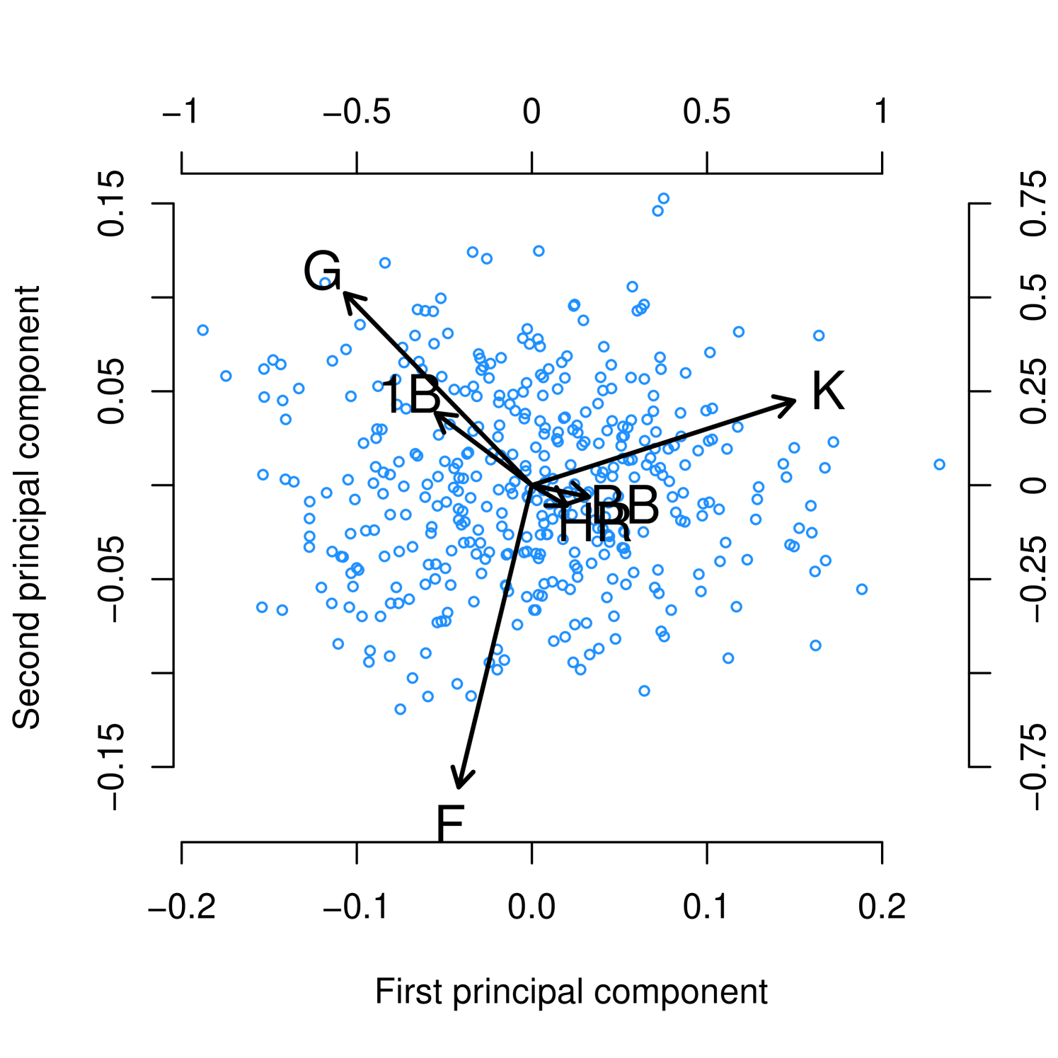
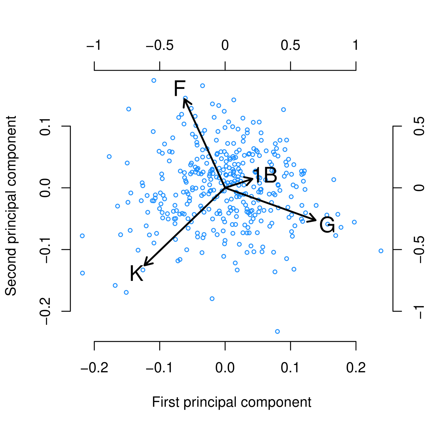
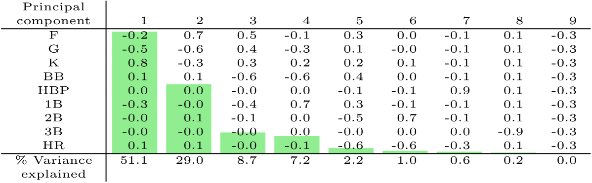
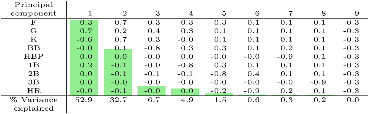
This structure is further evidenced by principal component analysis of the player-outcome matrix, illustrated in Figures 2 and 3. For batters, the principal component (PC) which describes most of the variance in observed outcome probabilities has negative loadings on all of the BIP outcomes and positive loadings on all of the TTO outcomes. For both batters and pitchers, the percentage of variance explained after two PCs drops off precipitously.
Principal component analysis is useful for illustrating the relationships between the outcome categories. For example Figure 3(a) suggests that batters who tend to hit singles (1B) more than average also tend to ground out (G) more than average. So an estimator of a batter’s groundout rate could benefit from taking into account the batter’s single rate, and vice versa. This is an example of the type of structure in outcome categories that motivates our proposal, which aims to leverage this structure to obtain better regression coefficient estimates in multinomial regression.
In Section 2 we review reduced-rank multinomial regression, a first attempt at leveraging this structure. We improve on this in Section 3 by proposing nuclear penalized multinomial regression, a convex relaxation of the reduced rank problem. We compare our method with ridge regression in a simulation study in Section 4. In Section 5 we apply our method and intepret the results on the baseball data, as well as another application. The manuscript concludes with a discussion in Section 6.
2 Multinomial logistic regression and reduced rank
Suppose that we observe data and for . We use to denote the matrix with rows , specifically . The multinomial logistic regression model assumes that the are, conditional on , independent, and that for
| (1) |
were and are fixed, unknown parameters. The model (1) is not identifiable because an equal increase in the same element of each of the (or in each of the ) does not the change the estimated probabilities. That is, for each choice of parameter values there is an infinite set of choices which have the same likelihood as the original choice, for any observed data. This problem may readily be resolved by adopting the restriction for some that and . However, depending on the method used to fit the model, this identifiability issue may not interfere with the existence of a unique solution; in such a case, we do not adopt this restriction. See the appendix for a detailed discussion.
In contrast with logistic regression, multinomial regression involves estimating not a vector but a matrix of regression coefficients: one for each independent variable, for each class. We denote this matrix by . Motivated by the principal component analysis from Section 1, instead of learning a coefficient vector for each class, we might do better by learning a coefficient vector for each of a smaller number of latent variables, each having a loading on the classes. For , this is the stereotype model originally proposed by Anderson, (1984), who observed its applicability to multinomial regression problems with structure between the response categories, including ordinal structure. Greenland, (1994) argued for the stereotype model as an alternative in medical applications to the standard techniques for ordinal categorical regression: the cumulative-odds and continuation-ratio models.
Yee and Hastie, (2003) generalized the model to reduced-rank vector generalized linear models. In detail, the reduced-rank multinomial logistic model (RR-MLM) fits (1) by solving, for some , the optimization problem:
| (2) | ||||
If rank, then there exist , such that . Under this factorization, the columns of can be interpreted as defining latent outcome variables, each with a loading on each of the outcome classes. The columns of give regression coefficient vectors for these latent outcome variables, rather than the outcome classes.
The optimization problem (2) is not convex because rank is not a convex function. Yee, (2010) implemented an alternating algorithm to solve it in the R (R Core Team,, 2016) package VGAM. However this algorithm is too slow for feasible application to datasets as large as the one motivating Section 1 (, , ).
3 Nuclear penalized multinomial regression
Because of the computational difficulty of solving (2), we propose replacing the rank restriction with a restriction on the nuclear norm (defined below) of the regression coefficient matrix. For some , this convex optimization problem is:
| (3) | ||||
We prefer to frame the problem in its equivalent Lagrangian form: For some ,
| (4) | ||||
This optimization problem (4) is what we call nuclear penalized multinomial regression (NPMR). We use to denote the log-likelihood of the regression coefficients and given the data and . The nuclear norm of a matrix is defined as the sum of its singular values, that is, the -norm of its vector of singular values. Explicitly, consider the singular value decomposition of given by , with and orthogonal and having values along the main diagonal and zeros elsewhere. Then
In the same way that the lasso induces sparsity of the estimated coefficients in a regression, solving (4) drives some of the singular values to exactly zero. Because the number of nonzero singular values is the rank of a matrix, the result is that the estimated coefficient matrix tends to have less than full rank. Thus (4) is a convex relaxation of the reduced-rank multiomial logistic regression problem, in much the same way as the lasso is a convex relaxation of best subset regression (Tibshirani,, 1996). The convexity of (4) makes it easier to solve than (2), and we discuss algorithms for solving it in Sections 3.1 and 3.2. In practice, we recommend using standard cross-validation techniques for selecting the regularization parameter , which controls the rank of the solution.
Consider the singular value decomposition of the estimated coefficient matrix . Each column of the orthogonal matrix represents a latent variable as a linear combination of the outcome categories. Meanwhile, each row of specifies for each predictor variable a coefficient for each latent variable, rather than for each outcome category. By estimating some of the singular values of (the entries of the diagonal matrix ) to be zero, we reduce the number of coefficients to be estimated for each predictor variable from (a) one for each of outcome categories; to (b) one for each of some smaller number of latent variables. These latent variables learned by the model express relationships between the outcomes because two categories for which a latent variable has both large positive coefficients are both likely to occur for large values of that latent variable. Similarly, if a latent variable has a large positive coefficient for one category and a large negative coefficient for another, those two categories oppose each other diametrically with respect to that latent variable.
3.1 Proximal gradient descent
NPMR relies on solving (4). The objective is convex but non-differentiable where any singular values of are zero, so we cannot use gradient descent. Generally, when minimizing a function of a vector , the gradient descent update of step size takes the form
or equivalently,
Still, if is non-differentiable, as it is in (4), then is undefined. However, if is the sum of two convex functions and , with differentiable, we can instead apply the generalized gradient update step (Hastie et al.,, 2015):
| (5) |
Repeatedly applying this update is known as proximal gradient descent (PGD). In (4), we have , and . So the PGD update step is:
where is the matrix containing the response variable and is the matrix containing the fitted values. That is, for , and ,
| (6) |
The problem is separable in and :
| (7) | ||||
| (8) | ||||
where is the soft-thresholding operator on the singular values of a matrix. Explicitly, if a matrix has singular value decomposition , then , where
is called the proximal operator of the nuclear norm, and in general solving (5) involves the proximal operator of , hence the name proximal gradient descent.
So to solve (4), initialize and , and iteratively apply the updates (7) and (8). Due to Nesterov, (2007), this procedure converges with step size if the log-likelihood is continuously differentiable and has Lipschitz gradient with Lipschitz constant . The appendix includes a proof that the gradient of is Lipschitz with constant , but in practice we recommend starting with step size and halving the step size if any proximal gradient descent step would result in an increase of the objective function (4).
3.2 Accelerated PGD
In practice, we find that it helps to speed things up considerably to use an accelerated PGD method, also due to Nesterov, (2007). Specifically, we iteratively apply the following updates:
-
1.
-
2.
-
3.
-
4.
The function in Step 3 returns the matrix of fitted probabilities based on the regression coefficients as described in (6). Step 2 is the key to the acceleration because it uses the “momentum” in to push it further in the same direction it is heading. We strongly recommend using this accelerated version of PGD, and our implementation of NPMR is available on the Comprehensive R Archive Network as the R package npmr.
3.3 Related work
The idea of using a nuclear norm penalty as a convex relaxation to reduced-rank regression has previously been proposed in the Gaussian regression setting (Chen et al.,, 2013), but we are not aware of any attempt to do so in the multinomial setting.
The nearest competitor to NPMR that can feasibly be applied to the baseball matchup dataset is multinomial ridge regression, which penalizes the squared Frobenius norm (the sum of the squares of the entries) of the coefficient matrix, instead of the nuclear norm. In detail, ridge regression estimates the regression coefficients by solving the optimization problem
| (9) |
This model is very similar to the state of the art in public sabermetric literature for evaluating pitchers on the basis of outcomes while simultaneously controlling for sample size, opponent strength and ballpark effects (Judge and BP Stats Team,, 2015). Software is available to solve this problem very quickly in the R package glmnet (Friedman et al.,, 2010). This is the standard approach used for regularized multinomial regression problems, so we use it as the benchmark against which to compare the performance of NPMR in Sections 4 and 5.
4 Simulation study
In this section we present the results of two different simulations, one using a full-rank coefficient matrix and the other using a low-rank coefficient matrix. In both settings we vary the training sample size from 600 to 2000, and we fix the number of predictor variables to be 12 and the number of levels of the response variable to be 8. Given design matrix and coefficient matrix , we simulate the response according to the multinomial regression model. Explicity, for , and ,
For both simulations the entries of are i.i.d. standard normal:
for . However the simulations differ in the generation of the coefficient matrix . In the full rank setting, the entries of follow an i.i.d. standard normal distribution: For ,
| (10) |
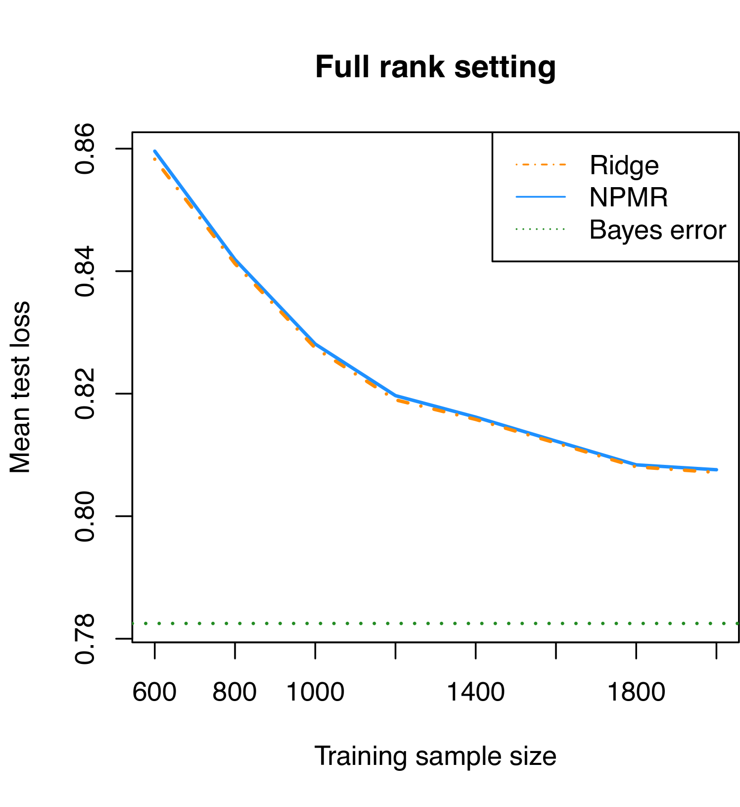
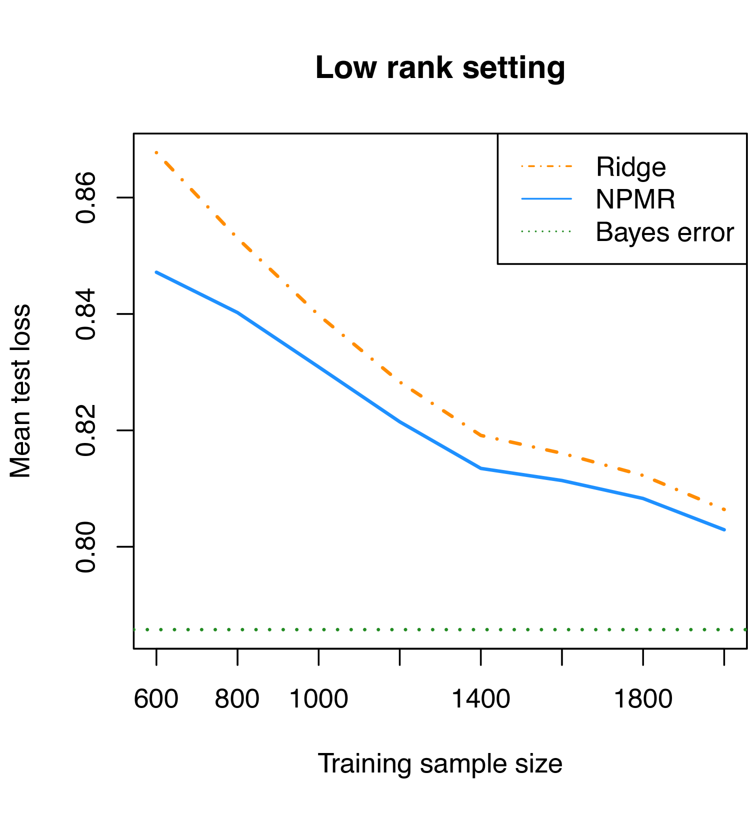
In the low rank setting we first simulate two intermediary matrices and with i.i.d. standard normal entries, and we then define so that the rank of is 2. In each simulation we fit ridge regression and NPMR to the training sample of size and estimate the out-of-sample error by simulating 10,000 test observations, comparing the model’s predictions on those test observations with the simulated response. The results of 3,500 simulations in each setting, for each training sample size , are presented in Figure 4.
In the full rank setting we expect ridge regression to out-perform NPMR because ridge regression shrinks all coefficient estimates toward zero, which is the mean of the generating distribution for the coefficients in the simulation. If this were a Gaussian regression problem instead of a multinomial regression problem, then the ridge regression coefficient estimates would correspond (Hastie et al.,, 2009) to the posterior mean estimate under a Bayesian prior of (10). In fact ridge regression does beat NPMR in this simulation (for all training sample sizes ), but NPMR’s performance is surprisingly close to that of ridge regression.
The low rank setting is one in which NPMR should lead to a lower test error than does ridge regression. NPMR bets on sparsity in the singular values of the coefficient matrix, and in this setting the bet pays off. The simulation results verify that this intuition is correct. NPMR beats ridge regression for all training sample sizes but especially for smaller sample sizes. By betting (correctly in this case) on the coefficient matrix having less than full rank, NPMR learns more accurate estimates of the coefficient matrix. As the training sample size increases, learning the coefficient matrix becomes easier, and the performance gap between the two methods shrinks but remains evident.
In summary, this simulation demonstrates that each of NPMR and ridge regression is superior in a simulation tailored to its strengths, confirming our intuition. Furthermore, in a simulation constructed in favor of ridge regression, NPMR performs nearly as well. Meanwhile NPMR leads to more significant gains over ridge regression in the low rank setting.
5 Results
5.1 Implementation details
The 2015 MLB play-by-play dataset from Retrosheet includes an entry for every plate appearance during the six-month regular season. For the purposes of fitting NPMR to predict the outcomes of PAs, the following relevant variables are recorded for the PA: the identity () of the batter; the identity () of the pitcher; the identity () of the stadium where the PA took place; an indicator () of whether the batter’s team is the home team; and finally an indicator () of whether the batter’s handedness (left or right) is opposite that of the pitcher.
For each outcome , the multinomial model fit by both NPMR and ridge regression is specified by
The parameters introduced have the following interpretation: is an intercept corresponding to the league-wide frequency of outcome ; corresponds to the tendency of batter to produce outcome ; corresponds to the tendency of pitcher to produce outcome ; corresponds to the tendency of stadium to produce outcome ; corresponds to the increase in likelihood of outcome due to home field advantage; and corresponds to the increase in likelihood of outcome due to the batter having the opposite handedness of the pitcher’s.
NPMR and ridge regression fit the same multinomial regression model and differ only in the regularizations used in their objective functions, yielding different results. See Section 3 for details. However there is a minor tweak to NPMR for application to these data. Instead of adding to the objective a penalty on the nuclear norm of the whole coefficient matrix, we add penalties on the nuclear norms of the three coefficient sub-matrices corresponding to batters, pitchers and stadiums. The coefficients for home-field advantage and opposite handedness remain unpenalized. The result is that NPMR learns different latent variables for batters than it does for pitchers, instead of learning one set of latent variables for both groups.
We process the PA data before applying NPMR and ridge regression. First, we define a minimum PA threshold separately for batters and pitchers. For batters the threshold is the -largest number of PAs among all batters. This corresponds roughly to the number of rostered batters at any given time during the MLB regular season. Batters who fall below the PA threshold are labelled “replacement level” and within each defensive position are grouped together into a single identity. For example, “replacement-level catcher” is a batter in the dataset just like Mike Trout is, and the former label includes all PAs by a catcher who does not meet the PA threshold. Similarly we define the PA threshold for pitchers to be the -largest number of PAs among all pitchers, and we group all pitchers who fall below that threshold under the “replacement-level pitcher” label. Additionally, we discard all PAs in which a pitcher is batting, and we discard PAs which result in a catcher’s interference or an intentional walk. The result is a set of 176,559 PAs featuring 401 unique batters and 362 unique pitchers in 30 unique stadiums.
5.2 Validation
We fit NPMR and ridge regression to the baseball data, using a training sample that varied from 5% (roughly 9,000 PAs) to 75% (roughly 135,000 PAs) of the data. In each case we used the remaining data to test the models, with multinomial deviance (twice the negative log-likelihood) as the loss function. For comparison we also include the null model, which predicts for each plate appearance the league average probabilities of each outcome. Figure 5 gives the results.
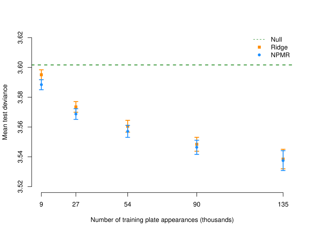
For each training sample size, NPMR outperforms ridge regression though the difference is not statistically significant. At the smallest sample size NPMR, unlike ridge regression, achieves a significanly lower error than the null estimator. There is value in improved estimation of players’ skills in small sample sizes because this can inform early-season decision-making. For all other sample sizes, both NPMR and ridge regression achieves errors which are statistically significantly less than the null error. The primary benefit of NPMR relative to ridge regression is the interpretation, as described in the next section.
5.3 Interpretation
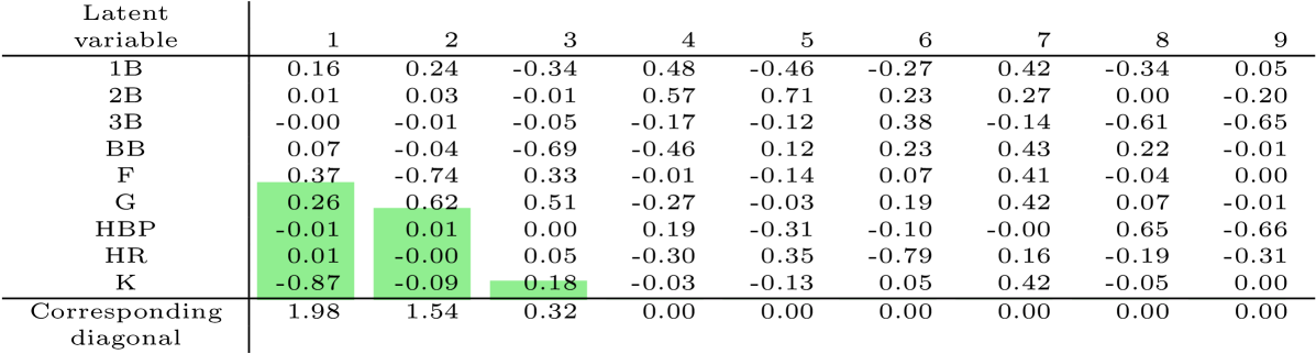
We focus on the results of fitting NPMR on 5 percent of the training data because there the difference between NPMR and ridge regression is greatest (Figure 5). As the sample size increases, the need for a low-rank regression coefficient matrix is reduced, and the NPMR solution becomes more similar to the ridge solution. Figure 6 visualizes the singular value decomposition of the fitted regression coefficient submatrices corresponding to batters and pitchers.
We observe that for both batters and pitchers, NPMR identifies three latent variables which differentiate players from one another. By construction, these latent variables are measuring separate aspects of players’ skills; across players, expression in each latent skill is uncorrelated with expression in each other latent skill. In that sense, we have identified three separate skills which characterize hitters and three separate skills which characterize pitchers. In baseball scouting parlance, these skills are called “tools”, but unlike the five traditional baseball tools (hitting for power, hitting for contact, running, fielding and throwing), the tools we identify are uncorrelated with one another.
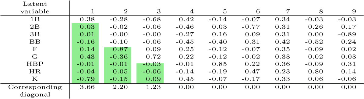
The interpretation of Figure 6 is very attractive in the context of domain knowledge. In reading the columns of , note that they are unique only up to a change in sign, so we can taken positive expression of each skill to mean positive or negative values of the corresponding latent variable. We suggest the following interpretation of the first three latent skills for batters:
-
•
Skill 1: Patience. The loadings of the first latent variable discriminate perfectly between the TTO outcomes and the BIP outcomes described in Section 1. We label this skill as “patience” because when a batter swings at fewer pitches, he is less likely to hit the ball in play.
-
•
Skill 2: Trajectory. The second latent variable distinguishes primarily between F and G, corresponding to the vertical launch angle of the ball off the bat.
-
•
Skill 3: Speed. The third latent variable distinguishes primarily between 1B and G. Examining the players with strong positive expression of this skill, we find fast players who are more difficult to throw out at first base on a ground ball.
From this interpretation we learn that the primary skill which distinguishes betwen batters is how often they hit the ball into the field of play. One outcome over which batters have relatively large control is how often they swing at pitches. Among balls that are put into play, batters have less but still subtantial control over whether those are ground balls or fly balls. It is the vertical angle of the batter’s swing plane, along with whether he tends to contact the top half or the bottom half of the ball, that determines his trajectory tendency. Finally, given the trajectory of the ball off the bat, the batter has relatively little control over the outcome of the PA. But to the extent that he can influence this outcome, fast runners tend to hit more singles and fewer groundouts.
Based on Figure 6, we interpret the pitchers’ skills as follows:
-
•
Skill 1: Power. The first latent variable distinguishes primarily between K and F (and G), thus identifying how the pitcher gets outs. Pitchers who tend to get their outs via the strikeout are known in baseball as “power pitchers”.
-
•
Skill 2: Trajectory. As with batters, the second latent variable distinguishes primarily between F and G, corresponding to the trajectory of the ball off the bat.
-
•
Skill 3: Command. The third latent variable distinguishes primarily between positive outcomes for the pitcher (F, G and K) and negative outcomes for the pitcher (BB and 1B), reflecting how well is able to control the location of his pitches.
The interpretation of the first two skills for pitchers is very similar to the interpretation of the first two skills for batters. Primarily, pitchers can influence how often balls are hit into play against them, but they exhibit less control over this than batters do. Secondarily, as with hitters, pitchers exhibit some control over the vertical launch angle of the ball off the bat. This is based on the location and movement of their pitches. The third skill, distinguishing between positive and negative outcomes, has a relatively very small magnitude.
| Skill | Patience | Trajectory | Speed |
|---|---|---|---|
| More K, BB | More F | More 1B | |
| Peter Bourjos | Ian Kinsler | Yoenis Cespedes | |
| Top | Eddie Rosario | Freddie Freeman | Lorenzo Cain |
| 5 | Carlos Santana | Omar Infante | José Iglesias |
| George Springer | Kolten Wong | Kevin Kiermaier | |
| Mike Napoli | José Altuve | Delino DeShields Jr | |
| Josh Reddick | Dee Gordon | Evan Longoria | |
| Bottom | JT Realmuto | Alex Rodriguez | Ryan Howard |
| 5 | AJ Pollock | Cameron Maybin | Odubel Herrera |
| Kevin Pillar | Shin-Soo Choo | Seth Smith | |
| Eric Aybar | Francisco Cervelli | Jake Lamb | |
| More F, G, 1B | More G, 1B | More G |
Table 1 lists the top five and bottom five players in each of the three latent batting skills learned by NPMR. These results largely match intuition for the players listed, and to the extent that they do not, it is worth a reminder that they are based on roughly nine days’ worth of data from a six-month season. The median number of PAs per batter in the training set is 21.
| Tool | Power | Trajectory | Command |
|---|---|---|---|
| More K | More F | More F, G, K | |
| José Quintana | Jesse Chavez | Max Scherzer | |
| Top | Corey Kluber | Justin Verlander | Masahiro Tanaka |
| 5 | Madison Bumgarner | Jake Peavy | Jacob deGrom |
| Max Scherzer | Johnny Cueto | Rubby de la Rosa | |
| Clayton Kershaw | Chris Young | Matt Harvey | |
| John Danks | Dallas Keuchel | Mike Pelfrey | |
| Bottom | Dan Haren | Garrett Richards | Chris Tillman |
| 5 | Cole Hamels | Sam Dyson | Eddie Butler |
| Alfredo Simón | Brett Anderson | Gio Gonzalez | |
| RA Dickey | Michael Pineda | Jeff Samardzija | |
| More F, G | More G | More BB, 1B |
The results in Table 2, listing the top and bottom players in each of the three latent pitching skills, are more interesting. The top five power pitchers are all among to top starting pitchers in the game. All the way on the other side of the spectrum is knuckleball pitcher RA Dickey. The knuckleball is a unique pitch in baseball thrown relatively softly with as little spin as possible to create unpredictable movement. Its goal is not to overpower the opposing batter but to induce weak contact. Another interesting pitcher low on power is Cole Hamels. Two of the leading sabermetric websites, Baseball Prospectus and FanGraphs, disagree greatly on Hamels’ value. The discrepancy stems from Baseball Prospectus giving full weight to BIP outcomes while FanGraphs ignores them. Because Hamels tends to get outs via fly balls and ground balls rather than strikeouts, FanGraphs estimates a much lower value for Hamels than Baseball Prospectus does.
5.4 Another application: Vowel data
Consider the problem of vowel classification from Robinson, (1989). The data set comprises 528 training samples and 462 test samples, each classified as one of the 11 vowels listed in Table 3, with 10 features extracted from an audio file. The data are grouped by speaker, with 8 subjects in the training set and 7 different subjects in the test set. Each audio clip is split into 6 frames during a duration of steady audio, yielding 6 pseudo-replicates.
| Vowel | Word | Vowel | Word | Vowel | Word | Vowel | Word |
|---|---|---|---|---|---|---|---|
| i | heed | A | had | O | hod | u: | who’d |
| I | hid | a: | hard | C: | hoard | 3: | heard |
| E | head | Y | hud | U | hood |
We fit NPMR and ridge regression to the training data over a wide range of regularization parameters, with the training and test loss (negative log-likelihood) reported in Figure 7. As the regularization parameter increases for each method, the training loss increases. The test loss initially decreases and then increases as the model is overfit. We observe that over the whole solution path, for the same training error NPMR consistently yields a lower test error than ridge regression.
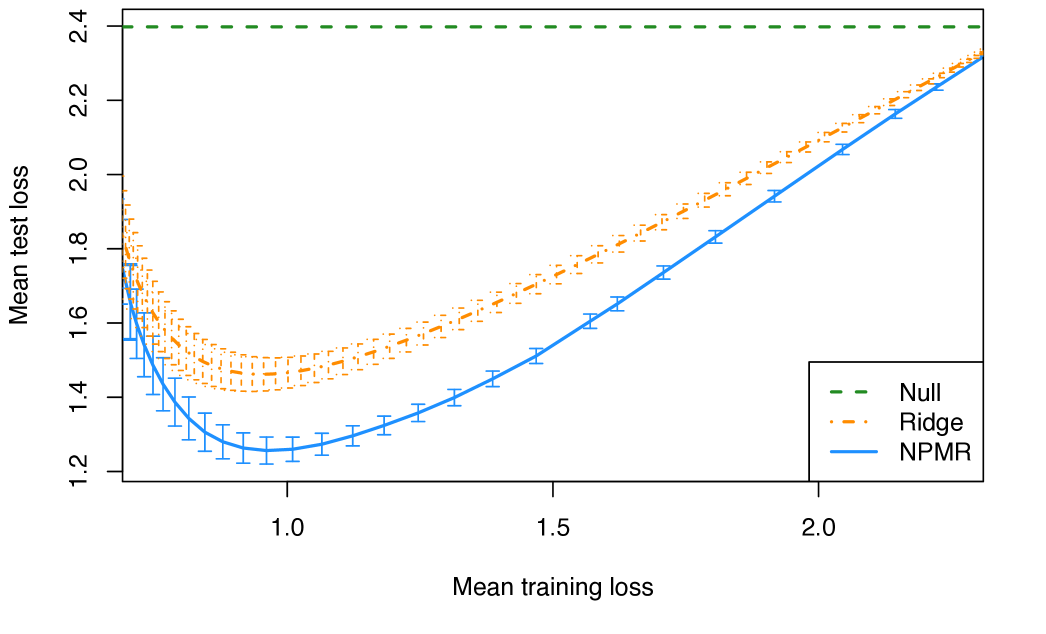
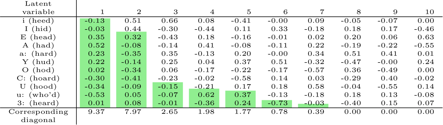
Figure 8 reveals a possible explanation why NPMR outperforms ridge regression on the vowel data. For example the results show that when the vowel i is a likely label, the vowel I is also a likely label. The first two latent variables explain a significant portion of the variance in the regression coefficients for the vowels. The first latent variable distinguishes between two groups of vowels, with C:, U and u: having the most negative values and E, A, a: and Y having the most positive values. NPMR has beaten ridge regression here by leveraging a hidden structure among response categories.
6 Discussion
The potential for reduced-rank multinomial regression to leverage the underlying structure among response categories has been recognized in the past. But the computational cost for the state-of-the-art algorithm for fitting such a model is so great as to make it infeasible to apply to a dataset as large as the baseball play-by-play data in the present work. Using a convex relaxation of the problem, by penalizing the nuclear norm of the coefficient matrix instead of its rank, leads to better results.
The interpretation of the results on the baseball data is promising in how it coalesces with modern baseball understanding. Specifically, the NPMR model has quantitative implications on leveraging the structure in PA outcomes to better jointly estimate outcome probabilities. Additional application to vowel recognition in speech shows improved out-of-sample predictive performance, relative to ridge regression. This matches the intuition that NPMR is well-suited to multinomial regression in the presence of a generic structure among the response categories. We recommend the use of NPMR for any multinomial regression problem for which there is some nonordinal structure among the outcome categories.
Acknowledgments
The authors would like to thank Hristo Paskov, Reza Takapoui and Lucas Janson for helpful discussions, as well as Balasubramanian Narasimhan for computational assistance.
References
- Albert, (2016) Albert, J. (2016). Improved component predictions of batting and pitching measures. Journal of Quantitative Analysis in Sports, 12(2):73–85.
- Anderson, (1984) Anderson, J. A. (1984). Regression and ordered categorical variables. Journal of the Royal Statistical Society B, 46(1):1–30.
- Baumer and Zimbalist, (2014) Baumer, B. and Zimbalist, A. (2014). The Sabermetric Revolution. University of Pennsylvania Press, Philadelphia.
- Bhatia, (1997) Bhatia, R. (1997). Matix Analysis. Springer, New York.
- Brown, (2008) Brown, L. D. (2008). In-season prediction of batting averages: A field test of empirical Bayes and Bayes methodologies. The Annals of Applied Statistics, 2(1):113–152.
- Chen et al., (2013) Chen, K., Dong, H., and Chan, K.-S. (2013). Reduced rank regression via adaptive nuclear norm penalization. Biometrika, 100(4):901–920.
- Efron and Morris, (1975) Efron, B. and Morris, C. N. (1975). Data Analysis Using Stein’s Estimator and its Generalizations. Journal of the American Statistical Association, 70(350):311–319.
- Friedman et al., (2010) Friedman, J., Hastie, T. J., and Tibshirani, R. J. (2010). Regularization paths for generalized linear models via coordinate descent. Journal of Statistical Software, 33(1):1–22.
- Grant et al., (2008) Grant, M., Boyd, S., and Ye, Y. (2008). CVX: A Language and Environment fo Statistical Computing. CVX Research.
- Greenland, (1994) Greenland, S. (1994). Alternative models for ordinal logistic regression. Statistics in Medicine, 13(16):1665–1677.
- Hastie et al., (2009) Hastie, T. J., Tibshirani, R., and Friedman, J. (2009). The Elements of Statistical Learning: Data mining, inference and prediction. Springer Series in Statistics. Springer, 2nd edition.
- Hastie et al., (2015) Hastie, T. J., Tibshirani, R. J., and Wainwright, M. (2015). Statistical Learning with Sparsity: The Lasso and its Generalizations. Monographs on Statistics and Applied Probability. CRC Press, 1st edition.
- Judge and BP Stats Team, (2015) Judge, J. and BP Stats Team (2015). DRA: An in-depth discussion. http://www.baseballprospectus.com/article.php?articleid=26196.
- Likert, (1932) Likert, R. (1932). A technique for the measurement of attitudes. Archives of Psychology, 140(22):1–55.
- Morris, (1983) Morris, C. N. (1983). Parametric Empirical Bayes Inference: Theory and Applications. Journal of the American Statistical Association, 78(381):47–55.
- Nesterov, (2007) Nesterov, Y. (2007). Gradient methods for minimizing composite objective function. Technical Report 2007076, Université Catholique de Louvain, Center for Operations Research and Econometrics (CORE).
- Null, (2009) Null, B. (2009). Modeling baseball player ability with a nested Dirichlet distribution. Journal of Quantitative Analysis in Sports, 5(2).
- R Core Team, (2016) R Core Team (2016). R: A Language and Environment fo Statistical Computing. R Foundation for Statistical Computing, Vienna, Austria.
- Robinson, (1989) Robinson, A. J. (1989). Dynamic error propagation networks. PhD dissertation, University of Cambridge.
- Tibshirani, (1996) Tibshirani, R. (1996). Regression shrinkage and selection via the lasso. Journal of the Royal Statistical Society B, 58(1):267–288.
- Yee, (2010) Yee, T. W. (2010). The VGAM package for categorical data analysis. Journal of Statistical Software, 32(10):1–34.
- Yee and Hastie, (2003) Yee, T. W. and Hastie, T. J. (2003). Reduced-rank vector generalized linear models. Statistical Modelling, 3(1):15–41.
Appendix A Appendix
Identifiability of multinomial logistic regression model
Hence and have the same likelihood. The ridge penalty in (9) provides a natural resolution. Any solution to this problem must satisfy
| (11) |
because otherwise can be replaced by with a smaller norm but the same likelihood and hence a lesser objective. Note that the optimization problem on the right-hand side of (11) is separable in the entries of and has the unique solution , meaning that the rows of in the solution must have mean zero. The unpenalized intercept stil lacks identifiability, but we may take it to have mean zero as well.
Similarly, the NPMR solution must satisfy
| (12) |
Whether this optimization problem always (for any ) has a unique solution is an open question. We speculate that it does and that the unique solution is . As evidence, each fit of NPMR in the present manuscript has a solution with zero-mean rows. As further evidence, we have used the MATLAB software CVX (Grant et al.,, 2008) to solve (12) for several randomly generated matrices , and each time the solution has been .
Note that must always be a solution to (12). To see this, note that
where is a projection matrix. Hence is also a projection matrix and has spectral norm (maximum singular value) . By Hölder’s inequality for Schatten -norms (Bhatia,, 1997),
so for any ,
In order words, the nuclear norm can always be decreased, or at least not increased, by centering the rows to have mean zero.
The problem with a lack of identifiability in the multimonial regression model comes in the interpretation of the regression coefficients. When comparing coefficients across variables for the same outcome class, it is concerning that an arbitrary increase in either coefficient can corresond to the same fitted probabilities (if that same increase applys to all other coefficients for the same variable). This does not apply to any of the interpretation in Section 5.3, but in the absence of certainty that there is a unique solution to (12), we take the NPMR solution to be the one for which the mean of and the row means of are zero.
Proof of Lipschitz condition for multinomial log likelihood
We prove that the multinomial log-likelihood from (4) has Lipschitz gradient with constant . Assume (without loss of generality) that the covariate matrix has a column of 1s encoding the intercept, so . The gradient of with respect to is given by , where and are defined as in (6). What we must show is that, for any :
| (13) |
Recall that is a function of , so corresponds to .
Consider a single entry of . Note that the gradient of with respect to is given by , where and
For any ,
This implies that the norm of the gradient of is bounded above by the inequality . So for any :
| (14) |
Now we are ready to prove (13).