Numerical approximation of a linear elasticity model
Abstract
We consider a nonlocal linear elastic wave model. We approximate the model using a spectral Galerkin method in space and analyze error in such an approximation. We perform some numerical experiments to demonstrate the scheme.
keywords: convolution integral; polynomial approximation; error estimate.
1 Introduction
Integro-differential equations arise while modeling many problems in physics, biology and other areas which involve non-local diffusion/dispersal mechanisms [2, 10, 11]. A nonlocal elastic wave model can be written as [11]
| (1) |
where
, is the time interval under consideration, is a time-independent coefficient and is an inhomogeneity. Here we consider , and , , where denotes the displacement field and represents velocity. Here the kernel satisfies (symmetry).
We assume that is a constant given by and for simplicity we consider a normalized kernel function (). Then (1) can be written as
| (2) |
where
Here we restrict ourself by (nonnegative) as well.
Now let , then . Considering [3] in (2) we have
Expanding in terms of Taylor series around we have
Thus we have
| (3) |
As is symmetric, integrals with odd powers of are zero. So (3) takes the form where ; for each Ignoring the higher order terms we have
| (4) |
The above equation is the familiar non-homogeneous wave equation, and is a first order approximation of the non-local equation (2). A comparison between the operators and is well presented in [3, 8]. Now following [3] it is well understood that is bounded and is negative semi-definite, if the kernel function is considered non-negative, symmetric and normalized. These properties are important for the analysis we performed in this study.
Emmrich et. al. [11] consider the non-local elastic model (2). They analyze mathematical and numerical solutions of the model. They compare the non-local model with that of a local continuum model. They claim two advantages of using this non-local model. They propose and implement a quadrature based numerical scheme considering infinite spatial domain.
It is well understood from [4, 9] that an integro-differential equation of type (2) defined in the infinite domain can also be defined in a truncated finite domain where and depend on the decay of the kernel function . It is to note that a closed form formula to find suitable and is well presented in [9]. Thus the analysis and the approximation in a periodic spatial domain can also be applied in any bounded interval (and vice-versa). Considering the kernel of the convolution integral as the author in [9] formulate and where considered so that .
One can consider the model in a spatial periodic domain [3] as well. If we consider a spatially one-periodic initial function , then for all and Then (2) can be written as
| (5) |
where for all , . We are interested to consider both periodic and non-periodic domain for spatial approximations of the model.
Convolution models have been extensively investigated both theoretically and numerically [5, 11], but a lot more yet to be done to get a highly accurate solver. Since an analytic solution can not be obtained always, an efficient and highly accurate numerical scheme has to be developed. Spatial approximation of this type of convolution models are interesting as well as challenging. The unknown function under integral sign and the nonlinearity involved in the model make the approximation more challenging. There are various ways to handle such problems. In most cases scientists use some lower order schemes (with midpoint quadrature rules for integration [3, 6]) to serve their purpose. Thus there is much room for improvement and we find an interest of presenting and analyzing a higher order technique for space integration. To the best of our knowledge, Legendre spectral Galerkin method has not been performed for this model problem yet and we find an interest to investigate such a scheme.
In this article, we start with numerical accuracy analysis of a spectral galerkin approximation in section 2 followed by numerical implementations of the scheme in section 3. We present several computer generated solutions with relevent discussion in section 4. We implement the schemes in MATLAB.
2 Accuracy of spectral Galerkin approximation
In this section, we look for spectral Galerkin scheme for space approximation and investigate convergence of such a scheme. Here we consider Legendre spectral polynomials. It is our goal to find , such that
and we seek for weak form to find such that
| (6) |
We denote be the set of all nonnegative integers. For any , denotes the set of all algebraic polynomials of degree at most in . We define Legendre spectral Galerkin approximation of (2) as: Find
| (7) |
We define projection operator such that
where
and
and
and denotes a nonnegative constant which is independent of .
Let be the error in spectral Galerkin approximation to the Legendre spectral Galerkin solution of (6). Now from (6) and (7) we have
| (8) |
Theorem 1.
We need the following results to prove Theorem 1.
Theorem 2.
[6] If , for all and with then is negative semi-definite.
Theorem 3.
[6] If , and then for any , is bounded and
3 Numerical implementation
Here we implement spectral Galerkin schemes considering Legendre spectral polynomials. The Legendre polynomials satisfy three term recurrence relation:
and
with
Here we consider for numerical implementations and one may extend the scheme to any interval , . We define
Replacing by in (6) we have
| (10) |
Now
and
where are Gauss weights and are Gauss quadrature points. We define
Now
where
and
Since we consider such that
we have
Adding all these integrals (10) can be written as
| (11) | |||||
for all . Thus (11) can be written as
with , and , and elements of are defined from the continuous operator as well as the elements of are defined from the continuous operator of . Since is a nonsingular diagonal matrix, the above second order ordinary differential equation can be written as
| (12) |
We approximate the integrals by Gaussian quadrature formula
and
where are quadrature points, and are quadrature weights. (11) is a system of second order time dependent ordinary differential equations which can be solved using a simple finite difference scheme to approximate the coefficients .
Depending on the nature of the kernel function, it is also wise to divide the integral domain into pieces. Then one can use small number of quadrature points to compute the integrals, since over each subinterval/subdomain will be flatter (if is a smooth function over .) We discuss the quadrature approximations in Section A.
4 Numerical experiments and discussion
In this section, we exhibit several numerical results to illustrate the scheme. Here we use a simple scheme for time integration. We use MATLAB to serve our purpose. We approximate the time dependent system of equations (12) using a central difference scheme 111Mathematica and MATLAB builtin functions can also be used to solve the time dependent system of equations (12).. For simplicity we consider and the scheme can be extended to , for any . We approximate (12) by
| (13) |
where This scheme is accurate [1] of order .
We know that for any matrix where stands for condition number of . Also Now
since
is a normalized function and . We have
and
Thus
and , shows that which is a bounded quantity for any finite . So as . Hence
and thus by the definition of condition number of a matrix
Thus the scheme (13) is unconditionally stable.
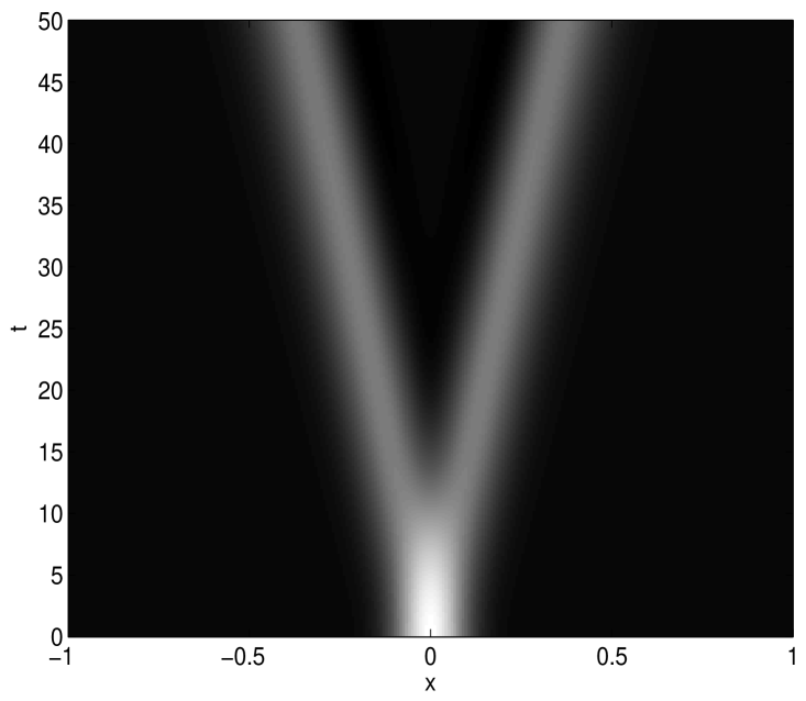
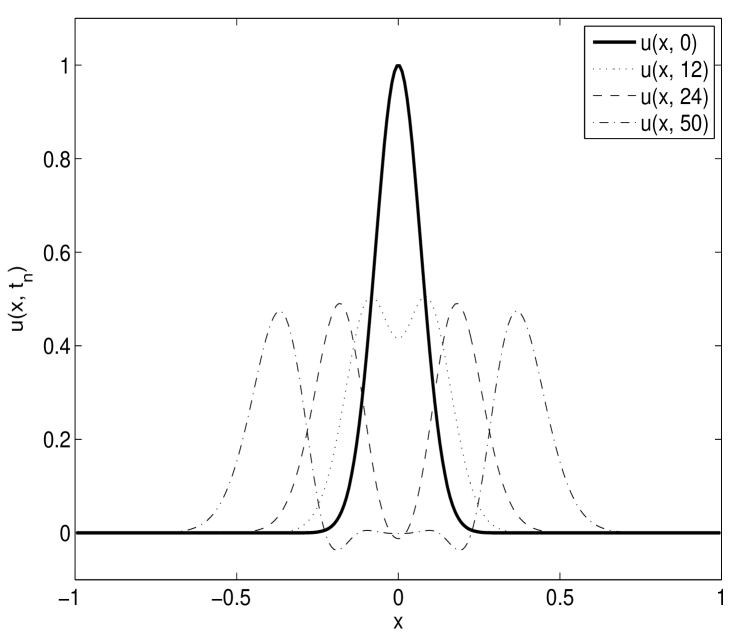
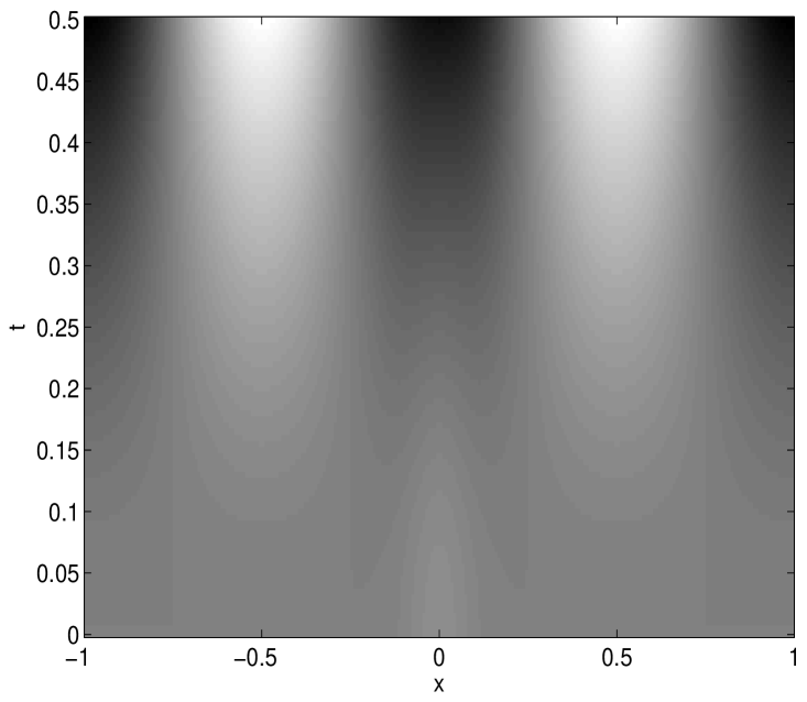
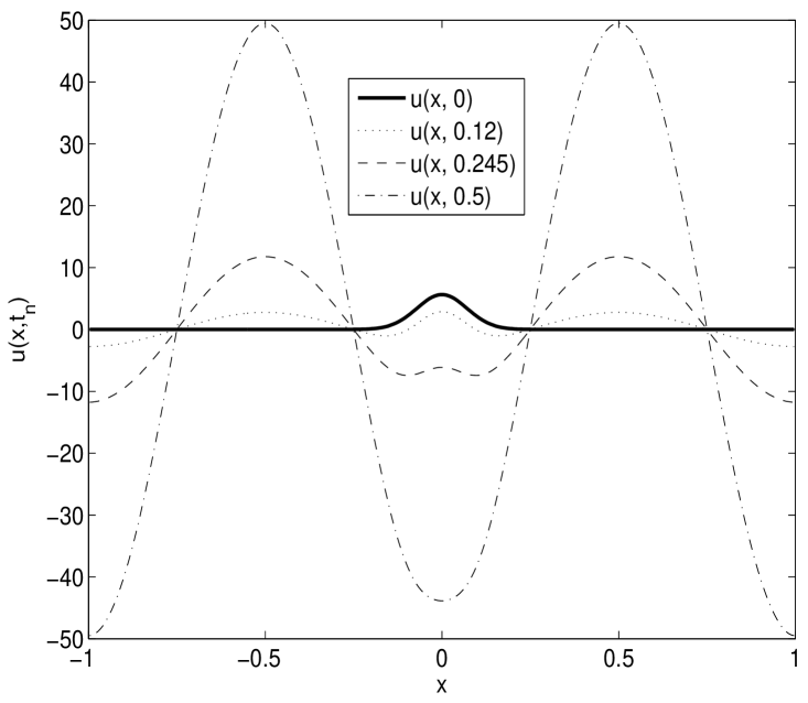
In the following Figures 1-2, we present the numerical solutions for various choices of initial functions, , and to demonstrate the scheme considering . Here we notice that the wave form is similar to the solutions of local linear wave model and the numerical solutions behaves well for any finite time preserving wave phenomena.
Here in this study we have shown theoretically that the error in spectral approximation decays exponentially. More precisely, it is shown that if the kernel function and the solution underlying the model problem is smooth, then the errors obtained by the Legendre spectral scheme decays exponentially, which one desires from spectral method.
There is a drawback of this approximation. Because of the presence of the convolution operator, the discrete operator is a dense matrix and as a result numerical computations become slower, needs huge storage for computations in multidimensional domain.
Appendix A Quadrature Approximation
We define , as quadrature points. Now in each point , we write (2) as
which can be approximated by
| (14) |
where are quadrature weights. (14) is a system of second order ordinary differential equations, which can be solved by any standard techniques.
One may also use a few quadrature points by subdividing the domain into several subdomains. We subdivide the domain into , subdomains such that . On each of the subdomains , we define points , as quadrature points.
Now in each point , we write (2) as
which can be approximated by point Gauss quadrature formula as
| (15) |
where are quadrature weights. (15) can be solved using any linear ordinary differential equation solvers.
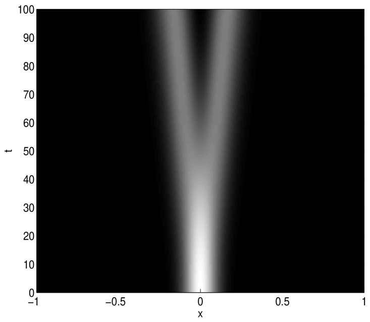
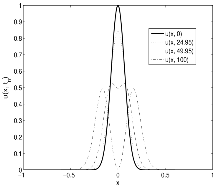
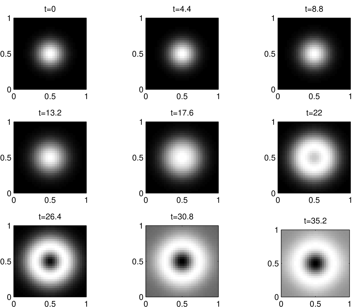
Here, in Figure 3, we demonstrate a solution of the model in two space dimensions using mid-point quadrature formula for space integration followed by Euler’s formula for time integration in a periodic space domain.
References
- [1] K. Atkinson and W. Han. Theoretical Numerical Analysis. Springer, 2001.
- [2] Peter W. Bates, Paul C. Fife, Xiaofeng Ren, and Xuefeng Wang. Travelling waves in a convolution model for phase transitions. Archive for Rational Mechanics and Analysis, 138(2):105–136, July 1997.
- [3] S. K. Bhowmik. Numerical approximation of a nonlinear partial integro-differential equation. PhD thesis, Heriot-Watt University, Edinburgh, UK, July, 2008.
- [4] S. K. Bhowmik. Numerical approximation of a convolution model of dot theta-neuron networks. Applied Numerical Mathematics, 61:581–592, 2011.
- [5] S. K. Bhowmik. Stability and Convergence Analysis of a One Step Approximation of a Linear Partial Integro-Differential Equation. Numerical methods for PDEs, 27(5):1179–1200, September 2011.
- [6] S. K. Bhowmik and D. B. Duncan. Piecewise Polynomial Approximation of a Nonlinear Partial Integro-Differential Equation. Technical report, Department of Mathematics, Heriot-Watt University, December, 2009.
- [7] C. Canuto, M. Y. Hussaini, A. Quarterni, and T. A. Zang. Spectral Methods, Fundamentals in Single Domains. Springer, 2006.
- [8] J. Carr and A. Chmaj. Uniqueness of travelling waves for nonlocal monostable equations. Proceedings of the American Mathematical Society, 132(8):2433–2439, Aug. 2004.
- [9] D. J. Duffy. Finite Difference Methods for Financial Engineering, A Partial Differential Equation Approach. Wiley Finance, John Wiley and Sons, 2006.
- [10] Dugald B. Duncan, M Grinfeld, and I Stoleriu. Coarsening in an integro-differential model of phase transitions. Euro. Journal of Applied Mathematics, 11:511–523, 2000.
- [11] Etienne Emmrich and Olaf Weckner. Anslysis and numerical approximation of an integro-differential equation modelling non-local effects in linear elasticity. Math. Mech. Solids, 12(4):363–384, 2007.
- [12] P. Solin, K. Segeth, and I. Dolezel. Higher Order Finite Element Methods. Chapman and Hall/CRC, 2004.