Numerical-experimental observation of shape bistability of red blood cells flowing in a microchannel
Abstract
Red blood cells flowing through capillaries assume a wide variety of different shapes owing to their high deformability. Predicting the realized shapes is a complex field as they are determined by the intricate interplay between the flow conditions and the membrane mechanics. In this work we construct the shape phase diagram of a single red blood cell with a physiological viscosity ratio flowing in a microchannel. We use both experimental in-vitro measurements as well as 3D numerical simulations to complement the respective other one. Numerically, we have easy control over the initial starting configuration and natural access to the full 3D shape. With this information we obtain the phase diagram as a function of initial position, starting shape and cell velocity. Experimentally, we measure the occurrence frequency of the different shapes as a function of the cell velocity to construct the experimental diagram which is in good agreement with the numerical observations. Two different major shapes are found, namely croissants and slippers. Notably, both shapes show coexistence at low () and high velocities () while in-between only croissants are stable. This pronounced bistability indicates that RBC shapes are not only determined by system parameters such as flow velocity or channel size, but also strongly depend on the initial conditions.
I Introduction
Red blood cells (RBCs) are the major constituent of mammalian blood and therefore determine the majority of its flow properties. One of the most amazing features of RBCs is their deformability, allowing them to squeeze through channels with diameters much smaller than their own equilibrium size Freund (2013); Picot et al. (2015); Salehyar and Zhu (2016). Another consequence of their deformability is the wide range of stationary and non-stationary shapes assumed by the RBCs in microchannel flows with dimensions similar to or slightly larger than the RBC equilibrium radius Fedosov et al. (2014); Aouane et al. (2014); Tahiri et al. (2013). Understanding and being able to predict these shapes is of high importance for a variety of reasons. From a fundamental point of view, it serves as the foundation in a bottom-up approach to understand the properties of red blood cell suspensions which are chiefly determined by single particle behavior Vitkova et al. (2008); Fedosov et al. (2011); Krüger et al. (2013); Thiébaud et al. (2014); Katanov et al. (2015); Lanotte et al. (2016). From an applied perspective, a series of recent investigations have devised promising approaches for sorting cells based on their mechanical properties either in lateral displacement devices Henry et al. (2016) or using high-speed video microscopy Otto et al. (2015). Finally, knowledge of the precise cell shape is also essential for accurately measuring geometric properties of cells Merola et al. (2017).
The most frequently observed shapes of RBCs in microchannel flows are the so-called “croissant” and “slipper” shapes. Examples are depicted in figure 1. Some researchers refer to croissants also as parachutes, although here we prefer the term croissant since our shapes are not perfectly rotationally symmetric (similar to the ones found by Farutin and Misbah (2014)). Probably one of the earliest experimental study on isolated red blood cells in flow was performed by Gaehtgens et al. Gaehtgens et al. (1980), where slippers as well as parachutes have been found depending on the diameter of the cylindrical channel. Suzuki et al. Suzuki et al. (1996) presented a phase diagram of parachutes and slippers as a function of velocity and confinement in a cylindrical tube. Slippers dominated at smaller diameters and higher velocities. Secomb et al. Secomb et al. (2007) compared experiments with 2D simulations in cylindrical channels of diameter for a cell velocity of approximately . Furthermore, two other publications Faivre (2006); Abkarian et al. (2008) considered the flow of RBCs at very low viscosity ratios of . They presented a phase diagram showing parachutes and slippers, where the velocity was varied in the very high regime of to . Tomaiuolo et al. Tomaiuolo et al. (2009) found parachutes at smaller and slippers at higher velocities in cylindrical channels of diameter. A subsequent study Tomaiuolo and Guido (2011) as well as Prado et al. (2015) considered the transient during start-up of the flow. Cluitmans et al. (2014) detected croissants at lower () and slippers at higher velocities () in rectangular channels with widths . Moreover, Quint et al. (2017) found a stable slipper and a metastable croissant at the same set of parameters in a wider channel of . Other publications presenting experiments in channel flow also touch the subject of RBC shapes but focus on other aspects such as the methodology Hochmuth et al. (1970); Seshadri et al. (1970); Zharov et al. (2006); Tomaiuolo et al. (2007); Guido and Tomaiuolo (2009); Gorthi and Schonbrun (2012); Lanotte et al. (2014); Tomaiuolo et al. (2016), dense suspensions and cell interactions Claver´ıa et al. (2016); Guest et al. (1963); Skalak and Branemark (1969); Gaehtgens et al. (1980); Kubota et al. (1996); Abkarian et al. (2008); Tomaiuolo et al. (2012); Wagner et al. (2013); Brust et al. (2014); Tomaiuolo et al. (2016) or use vastly larger channel diameters Goldsmith and Marlow (1972); Lanotte et al. (2016).
Numerical simulations and semi-analytical calculations of isolated particles in microchannels mostly studied axisymmetric RBCs Secomb et al. (1986); Secomb (1987); Secomb et al. (2001) or 2D vesicles Secomb and Skalak (1982); Kaoui et al. (2009a, 2011, 2012); Shi et al. (2012); Tahiri et al. (2013); Lázaro et al. (2014); Aouane et al. (2014). The numerical work by Aouane et al. (2014), for example, identified a large amount of dynamics including deterministic chaos. The first full 3D simulation of single cells with a realistic RBC model (but with a ratio of inner to outer viscosity of ) was conducted by Noguchi and Gompper Noguchi and Gompper (2005) who used a cylindrical tube with a diameter of . They found the typical discocyte shape below and parachutes above a critical velocity which depends on the elastic parameters. A subsequent study by the same group additionally explored this threshold as a function of confinement McWhirter et al. (2011). Moreover, Fedosov et al. Fedosov et al. (2014) presented very detailed phase-diagrams where the velocity and confinement was varied for three different sets of elastic moduli and a viscosity ratio of . They observed four distinct regions where snaking, tumbling, slippers and parachutes occurred. Recently, Ye et al. (2017) considered the shapes of an RBC with in rectangular microchannels (with width and aspect ratios to ) for the three cell velocities , and and observation times up to . Snapshots after this short initial transient showed parachutes or slightly slipper-like shapes.
Bistability, i.e. the observation of two different stable shapes depending on the initial condition but at otherwise identical system parameters, was barely considered so far. It was observed only numerically for simpler situations such as close-to-spherical vesicles in unbounded Poiseuille flow Farutin and Misbah (2014) or near a single wall Kaoui et al. (2009b), for a 2D RBC model in bounded Poiseuille flow Secomb et al. (2007), for the initial transient of a red blood cell in a rectangular channel Ye et al. (2017) or for simple shear flows Cordasco et al. (2014); Peng et al. (2014); Sinha and Graham (2015); Lanotte et al. (2016). No systematic experimental investigations exist for cells flowing in microchannels. Moreover, the 3D simulations and experimental investigations that were mentioned above and that consider the RBC shapes in microchannels in more detail all used a viscosity ratio of , although 2D simulations showed that choosing a physiologically more realistic value of Cokelet and Meiselman (1968) can significantly affect RBC dynamics Kaoui et al. (2012); Tahiri et al. (2013).
Here we present a detailed systematic experimental-numerical study on the steady-state shape of isolated red blood cells in a rectangular microchannel. We use the physiological viscosity ratio of appropriate for healthy human red blood cells in the microcirculation Cokelet and Meiselman (1968). The initial position is varied in the simulations directly, while experimentally we determine it via measurements at the channel entrance. Our central finding is that the initial starting position of the RBC has a decisive influence on the final steady-state shape of the red blood cell.
II Methods
II.1 Experimental setup
The sample preparation and experimental setup is mostly identical to the one used recently by Claver´ıa et al. (2016). In short, human red blood cells were obtained from healthy donors by needle-prick and used within three hours. After appropriate preparation Claver´ıa et al. (2016), they are suspended in a phosphate buffered saline (PBS) and bovine serum albumin solution which has a viscosity of approximately . The viscosity ratio of the cells is therefore Quint et al. (2017). This value corresponds to the typical physiological value of healthy red blood cells in blood plasma Cokelet and Meiselman (1968). The RBCs are pumped through rectangular, PDMS-based channels by a high-precision pressure device (Elveflow OB 1, MK II) with pressure drops ranging from to at room temperature. The channels have a cross-section width of and a height of without any applied pressure drop and are thus similar to the vessel diameters found in the microvascular system Popel and Johnson (2005). We use rectangular rather than cylindrical channels since they are easier to manufacture, are therefore prevalent in lab-on-a-chip devices and have the merit that cells are not rotated randomly around their axis due to the missing rotational symmetry. The latter property greatly simplifies the microscopic observation and analysis of the RBCs.
The hematocrit (volume percentage of RBCs) in the reservoir before the inlet is always , i.e. very low. Nevertheless, we find cells flowing in clusters as well as single cells. For the present work we have analyzed only the latter. To this end, previous experimental and theoretical results showed that the hydrodynamic interaction in a linear channel decays exponentially, and becomes negligible if the inter-particle distance is more than twice the channel width Cui et al. (2002); Diamant (2009); McWhirter et al. (2011). Considering that our channel has the dimensions , cells can be considered as being single for distances . We only used cells that were at least apart from other entities.
We perform measurements at two locations along the channel, namely at the entrance () and at downstream. Vessel lengths in-between bifurcations in the microvascular system are less than , i.e. much shorter Koller et al. (1987). Nevertheless, this is not necessarily true for in-vitro experiments or lab-on-a-chip devices, and the long-time behavior also holds information about the general intrinsic properties. The flowing RBCs are recorded by an inverted bright-field microscope (Nikon TE 2000-S) with an oil-immersion objective (Nikon CFI Plan Fluor , ) and a high-resolution camera (Fastec HiSpec 2G) at a frame rate of 400 frames per second. The camera is aligned along the -direction so that the photographs show the cells in the --plane (compare figure 2). Hence, determination of the -position is not possible, but also not absolutely necessary as our simulations always show a -position of nearly (see section V). We analyze the recorded image sequence with a custom MATLAB script that detects each projected cell shape and the corresponding 2D center of mass position. It additionally tracks the cell position over the image sequence to obtain the individual cell velocity. Considering the optical setup, we assume an uncertainty in the position measurements of with .
II.2 Simulation setup
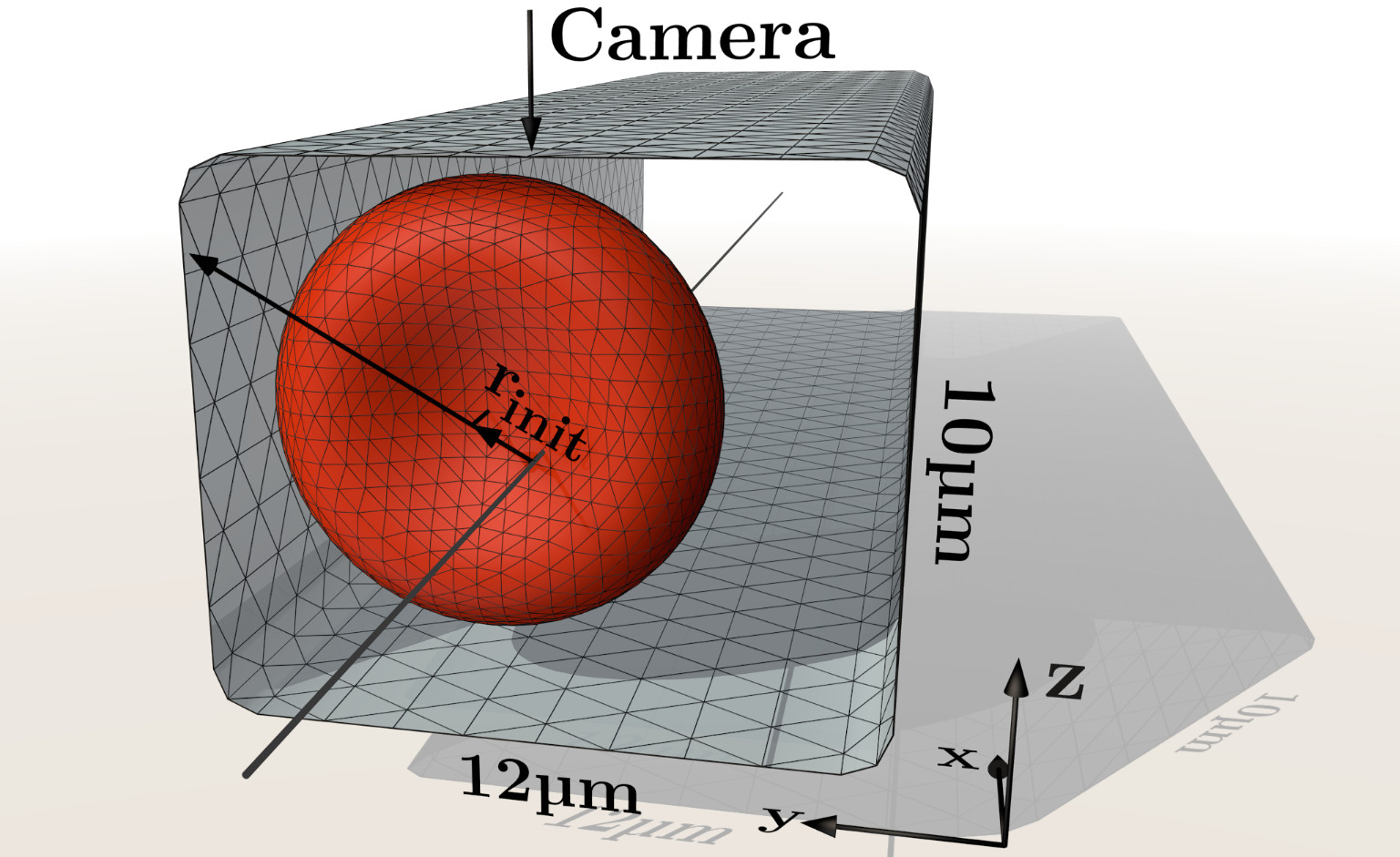
The numerical simulations mimic our experimental setup as far as possible. Hence, we place a single red blood cell in a rectangular channel as shown in figure 2. The channel has a cross-section of width and height . Periodic boundary conditions are assumed in the -direction with a periodicity of , in agreement with above estimates for the decay of hydrodynamic interactions.
We vary the initial --position (relative to the channel center) of the RBC’s centroid along the line , which almost corresponds to the channel diagonal. The corresponding initial radial position is thus simply given by . When starting with the typical discocyte equilibrium shape Evans and Fung (1972); Le (2010), as depicted in figure 1(a), the RBC axis is aligned with the channel axis (as shown in figure 2). Cell velocities are extracted by considering the difference of the centroids between successive time steps. During the simulation, we monitor several quantities such as the radial, - and -positions, the RBC asphericity or the cell velocity as well as the full 3D shape to determine when a steady state has been reached.
Regarding the actual modeling of the constituents, the RBC is filled with a Newtonian fluid with a dynamic viscosity , whereas the ambient flow is a Newtonian fluid with the dynamic viscosity of blood plasma Chien et al. (1966); Skalak et al. (1989); Secomb (2017). We set the viscosity ratio to a value of in all simulations. The surface area of the RBC is set to and the volume is set to (see e.g. references 67 and 69), leading to a large radius of when the cell is in the typical discocyte equilibrium shape (figure 1(a)). The mechanics of the infinitely thin membrane are governed by Skalak’s law Skalak et al. (1973); Krüger et al. (2011) for the in-plane elasticity with a shear modulus of Yoon et al. (2008); Freund (2014) and an area dilatation modulus of . This value for ensures that the area changes remain below in all cases. We take the reference state for the Skalak model to be the typical discocyte shape Evans and Fung (1972); Le (2010). The membrane is additionally endowed with some bending resistance which is modeled according to the Canham-Helfrich law Canham (1970); Helfrich (1973); Guckenberger and Gekle (2017a), where the bending modulus is fixed to Park et al. (2010); Freund (2014). The spontaneous curvature is set to zero.
We use 2048 flat triangles to discretize the RBC in our numerical implementation. The forces are computed as described by Guckenberger et al. (2016), with Method C therein being used for the bending contribution. An unavoidable artificial volume drift of the cell is countered by adjusting the velocity to obey the no-flux condition and by a subsequent rescaling of the object Farutin et al. (2014); Guckenberger and Gekle (2017b). Moreover, the channel is represented by 2166 flat triangles. The corners are rounded to prevent numerical problems (compare figure 2). Rather than prescribing a zero velocity at the channel walls, we use a penalty method for efficiency reasons with a spring constant of Guckenberger and Gekle (2017b); Tahiri et al. (2013). Increasing the triangle counts and the box length did not change the results significantly.
The Reynolds number in the considered system is defined as . For a velocity of and the density of the ambient and inner liquid we therefore have . Hence, the flow can be appropriately described using the Stokes equation. This allows us to employ the boundary integral method (BIM) Pozrikidis (2001) for 3D periodic systems Guckenberger and Gekle (2017b); Zhao et al. (2010). Note that this method requires to prescribe a certain average flow through the whole unit cell instead of a pressure drop within the channel. The latter is unfortunately not easily accessible. We therefore compare with experiments by means of cell velocities. Continuing, the integrals are computed by a standard Gaussian quadrature with points per triangle in conjunction with linear interpolation of nodal quantities and appropriate singularity removal for the single- and double-layer potentials Guckenberger and Gekle (2017b). Furthermore, we use the smooth particle mesh Ewald (SPME) method Saintillan et al. (2005) to accelerate the computation of the periodic Green’s functions; cutoff errors are kept below . The resulting linear system is solved via GMRES Saad and Schultz (1986) up to a residuum of , and the kinematic condition is integrated in time using the adaptive Bogacki-Shampine algorithm Bogacki and Shampine (1989) with the absolute tolerance set to . When the run-times are normalized to a two-socket system with 28 cores, each simulation took 1 to 29 days, with an average of around 5 days. The phase diagrams below are formed by 329 of such simulations in total. Further details on the numerical method as well as verifications of the implementation can be found in our previous publications Guckenberger and Gekle (2017b); Guckenberger et al. (2016); Daddi-Moussa-Ider et al. (2016); Quint et al. (2017).
III Experimental results
We classify cells in the experiments either as croissants, slippers or “other” not uniquely identifiable or completely different shapes. Typical slipper and croissant shapes are shown in the photographs (b) and (e) of figure 1. See the supplementary information (SI) for a collection of all images.
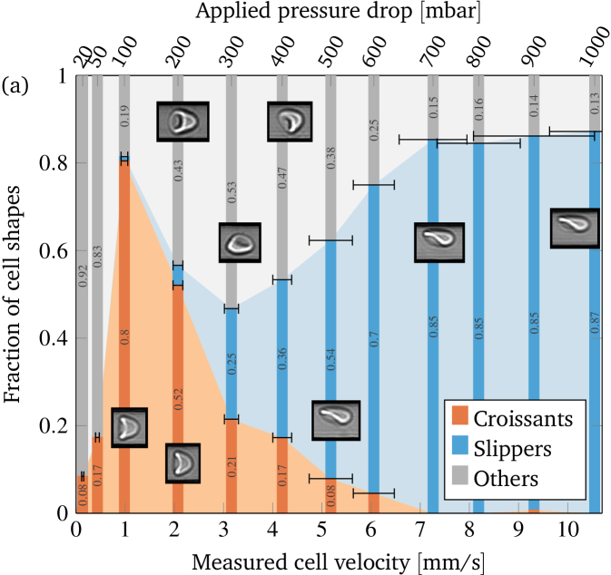
To systematically investigate the occurrence of the different shapes, we vary the imposed pressure drops from 20 to . The corresponding cell velocities range from to , covering the whole physiological range in microchannels Pries et al. (1995); Popel and Johnson (2005); Baskurt et al. (2011). We consider the cells away from the channel entrance where most of the cells reached a steady state Claver´ıa et al. (2016). Figure 3(a) depicts the fraction of observed shapes as a function of the measured cell velocities, constituting our central result from the experiments. This distribution was obtained by considering typically more than 100 cells per imposed pressure drop. The average velocities were computed by averaging over all cells at a certain pressure drop, with the horizontal error bars showing the corresponding standard deviations in cell velocity. Not all velocities are the same because croissants and slippers have different velocities at otherwise identical flow conditions Quint et al. (2017), and because of the natural variations of cell properties such as elasticity and size, as also noted by Tomaiuolo et al. (2009). See the supplementary information for more details. Considering figure 3(a), high velocities obviously favor slippers while croissants are the most prominent for medium velocities. A pronounced peak exists from around to . Very small velocities produce mostly shapes that fall outside our simple two-state classification.
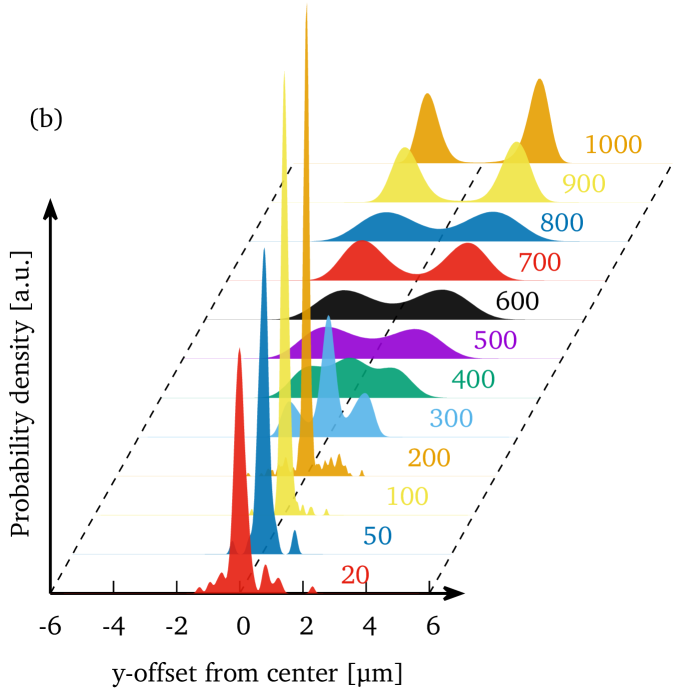
Figure 3(b) illustrates the corresponding estimated probability density function of the center of mass -position of the cells at the various pressure drops.
This estimate was obtained from the measured -positions by using the kernel density estimator as implemented in MATLAB R2017a (ksdensity) with a support of and otherwise default settings.
Thus, croissants and “others” occurring at lower velocities are centered in the channel, while slippers occurring at high velocities show a pronounced off-centered position.
The assumed shapes therefore imply a certain -position within the channel with slippers being off-centered and croissants centered.
This is confirmed when analyzing the offset distribution separately for each shape class as shown in the supplementary information.
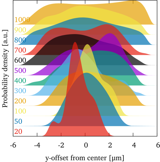
From figure 3(a) it is tempting to conclude that the flow velocity is the major parameter that determines the RBC shape with low velocities favoring centered and high velocities favoring off-centered flow positions. However, looking at the cell positions near the channel entrance (figure 4) we find that already upon entering the channel RBCs are not homogeneously distributed. At low velocities we observe a clear bias towards a centered initial position, with the distribution becoming approximately homogeneous only at the highest measured velocities. These experimental observations allow two distinct parameters as the reason for the dominance of the slipper shapes at high velocities: either the higher flow velocity itself or the more off-centered entry into the channel. To disentangle these two possibilities we now present numerical simulations whose geometry directly corresponds to the experimental setup.
IV Numerical results
We numerically study the behavior of a single RBC in a rectangular microchannel by varying the imposed flow velocity, the initial shape and the initial offset from the centerline of the tube (see section II.2). After starting the flow, we wait until the RBC reaches the steady state where the shape as well as the radial position does no longer change, or alternatively until periodic motion is observed.
In the majority of cases, we observe two different states: A croissant shape (which moves as a rigid body, figure 1(c)) and a slipper shape (figure 1(f)). The latter exhibits tank-treading (TT) and oscillatory contractions similar to the slippers seen by Fedosov et al. (2014) (see the SI for a movie and the insets in figure 5). Tank-treading refers to the motion of the membrane around a (more or less) static shape. Note that perfectly axisymmetric parachutes are suppressed by the rectangular channel flow, contrary to the situation for cylindrical tubes Fedosov et al. (2014) or unbounded Poiseuille flows Farutin and Misbah (2014).
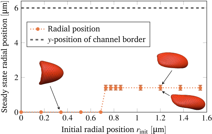
To start the systematic study, we take a red blood cell that is initially in the typical discocyte shape with its rotation axis aligned along the tube’s axis (cf. fig. 2). We then vary the radial offset from the center line as described in section II.2 and record the final radial position as well as the shape. The mean of the radial position is extracted by a temporal average once the cell is in the steady state (see the supplementary information for more details). Figure 5 shows the result for a cell velocity of . A single sharp transition at from centered croissants to off-centered slippers is observed. The final position of the slippers is mostly offset only along the wider width of the channel (-direction), but not along the smaller height (-direction). Hence we find pronounced bistability: The result is significantly determined by the initial condition and two different shapes coexist. This is consistent with the 2D simulations by Secomb et al. Secomb et al. (2007) and Tahiri et al. Tahiri et al. (2013). It also agrees qualitatively with observations by Farutin and Misbah for 3D simulations of vesicles in unbounded Poiseuille flow Farutin and Misbah (2014).
To study the bistability in more detail, we vary the imposed flow velocity as well as the initial offset and characterize the behavior in the steady state. This yields the shape phase diagram depicted in figure 6(a). The cell velocity is extracted in the steady state via a temporal average. For slippers the velocity varies periodically (similar to the radial position): the minimum and maximum in one period is indicated by the horizontal error bars. Overall, the mean cell velocity ranges from to , matching with the experimentally covered range. The corresponding shear capillary number varies therefore in the interval , while the bending capillary number lies in the range . The reddish area illustrates the approximated region where croissants exist. Furthermore, there is a maximal initial offset above which overlapping with the vessel wall would occur.
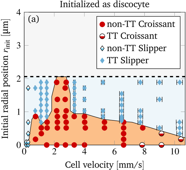
The shape phase diagram in figure 6(a) (together with (b) and (c) explained below) constitutes our main result from the simulations. Starting near the channel center (in the reddish region) results in croissants, whereas higher initial offsets lead to slippers. The transition is found to be sharp, and depends significantly on the velocity. Croissants are the only stable steady state in a small region ranging from around to , independently of the initial radial position. Smaller and larger velocities tend to favor slippers. Stable croissants do not appear below . In the case of the slippers, the final periodic state is usually reached after roughly to . In contrast, the final croissant state is sometimes achieved only after more than to , possibly after an intermediate slipper state that can last several seconds (see figure S4 and the movie in the supplementary information). Hence, shapes observed after less than one second often turn out to be transient, contrary to the interpretation of Ye et al. (2017) but in agreement with Prado et al. (2015).
Considering our results in figure 6(a) in more detail, we find that two different types of croissants and slippers are possible. On the one hand, at very low velocities () the slippers no longer exhibit tank-treading motion of the membrane and instead show tumbling behavior: The cell rotates around the -axis while approximately preserving its shape (similar to a rigid-body, see the SI for a movie). The difference compared to the tumbling motion observed by Fedosov et al. (2014) is that the cell still exhibits a clear slipper-like instead of a proper discocyte shape. Hence, we classify this mode still as slipper. On the other hand, at very high velocities () slightly asymmetric shapes strongly reminiscent of croissants with a distinct tank-treading motion can sometimes be observed (see the inset in figure 6(c) for an example). As the shape itself is very close to a croissant, we will nevertheless consider it to be a croissant below.
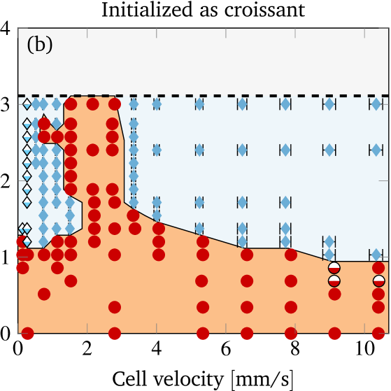
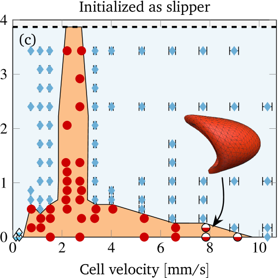
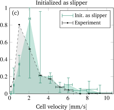
A natural question that occurs in light of the profound bistability is the influence of other initial shapes on the result. To this end, we consider a typical croissant as well as a typical slipper as the starting shape. Both were obtained from previous simulations that started with the discocyte form and are depicted in the supplementary information. We once again construct the shape phase diagram as before and display the results in figures 6(b) and (c). Note that the different starting shapes admit a larger initial radial position of the centroid. In short, starting with a croissant favors croissants in the steady state (the reddish area is larger than in figure 6(a)). For slippers it is the other way around: Starting with a slipper tends to produce more slippers (reddish area smaller than in figure 6(a)). Despite this, the croissant-only region from around to still exists unscathed. Overall, only two qualitative differences occur between the phase diagrams of different initial shapes, both at lower velocity when starting with the croissant shape (figure 6(b)): First, stable croissants emerge at very low velocities () and second, the croissant-only peak exhibits a “protrusion” into the slipper space. This observation suggests that slippers and croissants can be stable below for most values, although in some cases a very precise croissant configuration is required in order to actually get a croissant in the steady state.
Another interesting aspect concerns the radial positions of the centroids in the final steady states. The average values are obtained by computing the temporal average in the steady state first for each simulation, and then combining the results for identical shapes via a weighted arithmetic mean. We use the observation time in the steady state as the weight. This procedure leads to figure 7(a). Obviously, the final radial positions are independent of the initial starting shape, i.e. a particular steady state shape at a certain velocity is always located at the same position. Furthermore, non-tank-treading croissants are always almost centered, with only minor deviations away from zero. These slight deviations in the range from 2 to are mainly due to some croissants exhibiting minuscule periodic shape deformations. Moreover, the centroids of tank-treading croissants occurring at velocities are located near but not directly in the center. Their slight off-centered position is a result of their asymmetry.
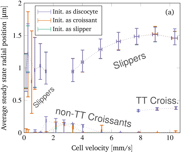
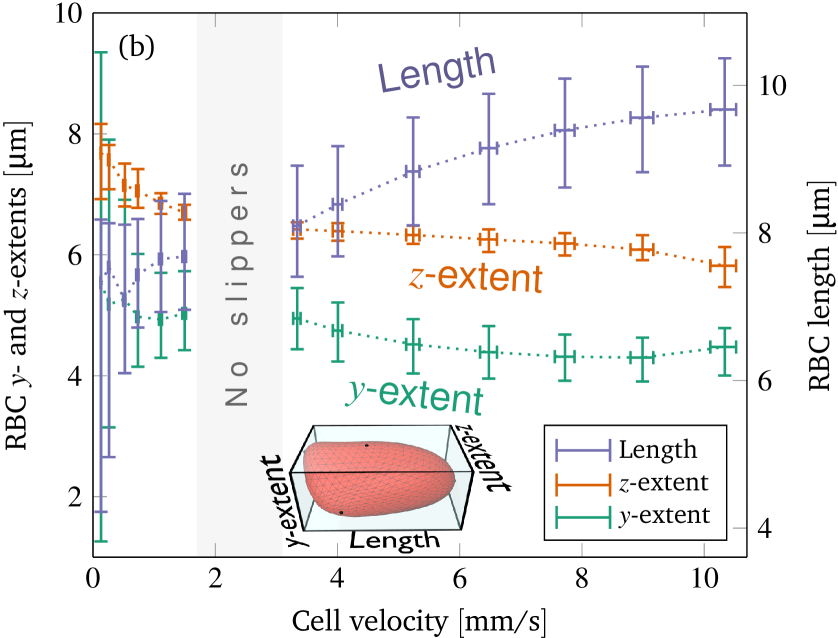
In contrast to croissants, slippers are located to away from the channel’s axis. The minimum position is attained for velocities near the border of the croissant-only region in the phase diagram (at around and , compare figure 6). Above, the off-center position increases and seems to converge to a value of around . The reason for this increase is that slippers become more elongated and thinner at higher velocities (up to a certain degree), as shown in figure 7(b) and also observed in previous experiments Tomaiuolo et al. (2009). Thus, they effectively become smaller in the radial direction and their centroids can move closer to the wall. We note that the distance between the wall and the upper side of the slipper approximately remains the same for all velocities. This also hints at that the “optimal” off-center position for the slippers is more than away from the center, and that this particular value is due to the smallness of the channel.
V Comparison between experiments and simulations
V.1 Comparison of shapes
Considering figure 1, the croissants obtained from simulations and experiments look very similar, although the experimental shapes appear to be somewhat larger. The reason is diffraction: The “true” cell border lies in the bright and not within the dark rim. However, the slippers appear to look qualitatively different. This is due to the high magnification and numerical aperture of the objective which results in a small depth of field of around . Cell borders above and below the middle plane are therefore blurred out and become invisible while the mid-plane cut becomes dominant. Thus, for comparison we should use the middle cross-section of the numerically obtained shapes. Here we find good agreement (compare figure 1(g) with (e)).
V.2 Comparison of the phase diagrams
A qualitative comparison between the phase diagrams of steady states from the experiments (fig. 3(a)) and the simulations (fig. 6) shows a striking resemblance: Both exhibit a distinct peak in the number of croissants at lower velocities (1 to ) at the expense of the number of slippers. The latter dominate the picture at high velocities (). At intermediate velocities both shapes coexist and can therefore be observed simultaneously in measurements. Moreover, the simulations at very low velocities showed croissants only if the initial RBC was already prepared in that state, meaning that in the experiments this shape is highly unexpected. Indeed, we were not able to clearly classify most of the observed shapes in that regime as either croissants or slippers.
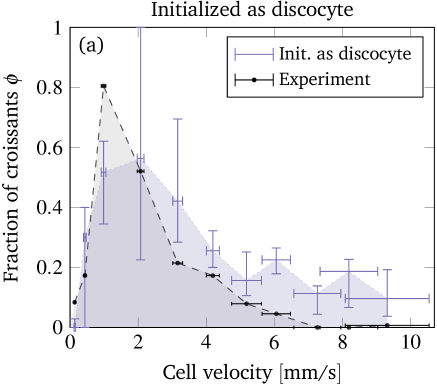
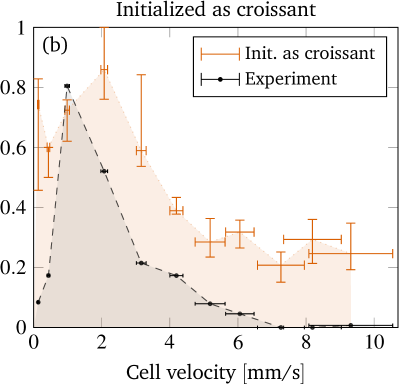
Obtaining a direct quantitative comparison requires a translation of the numerical threshold in figure 6 (which is in terms of the initial offset) into a prediction regarding the fraction of shapes, because the experimental phase diagram is in terms of the observed fraction of shapes. This is done by counting the fraction of croissants entering the channel with an offset below the numerical threshold. This fraction corresponds directly to the predicted fraction of croissant shapes. More precisely, we first define as the initial radial offset which separates croissants from slippers in the simulations by using the black line in figure 6. An exception is the small croissant-only region (i.e. the interval of the topmost horizontal line in figure 6) where we take . This is consistent with our interpretation that only croissants exist in this particular interval. One is computed for each experimental cell velocity from figure 3 (a). Second, each radial position is projected onto the -axis to give (see sec. II.2) because only the -offset is known from experiments. Third, from the experimental offset distribution at the channel entrance (figure 4) we can then estimate the fraction of cells that enter the channel with an offset below . Accordingly, the simulations predict a fraction of croissants in the steady state. The value of can thus be directly compared with the experimental phase diagram from figure 3 (a). This is done once for every starting configuration employed in the simulations.
Figure 8 shows this key result of our contribution, i.e. the predicted fraction of croissants as a function of the cell velocity for each starting shape. The vertical error bars depict the uncertainty in the prediction, whose computation is explained in the supplementary information. They are comparably large in the croissant-only region because the experimental velocities lie very near its sharp boundary. The horizontal error bars illustrate the standard deviation of the experimentally measured cell velocities. Clearly, we find very good agreement between the prediction from the simulation and the experimental observation when considering the slipper starting shape (figure 8(c)). Starting with a discocyte or croissant leads to slightly more pronounced deviations (figures 8(a) and (b)), but still a satisfactory semi-quantitative agreement is maintained. This suggests the intuitive conclusion that the starting shapes in the experiment are closer to the rather asymmetric slippers than to the highly symmetric discocytes or croissants. Indeed, as explicitly shown in the SI, we only observe non-classifiable and rather asymmetric “other” shapes at the channel entrance.
As mentioned in the introduction, experimental investigations with more detailed shape studies are rather scarce. A comparison of the phase diagrams with the experimental literature is therefore limited to rough qualitative statements. Tomaiuolo et al. (2009) found croissants and “others” for a cell velocity of using in a cylindrical tube with diameter . This is in agreement with our results. At , slippers but also croissants have been observed. Since we cannot reach velocities that high, we can neither confirm nor refute the occurrence of the latter. Extrapolation of figure 8 is dangerous since the Reynolds number at is around and thus inertia effects might have noticeable contributions Kaoui and Harting (2016); Schaaf and Stark (2017). Continuing, Cluitmans et al. (2014) found croissants and tumbling “others” at and slippers at in rectangular channels of and widths and a height of , which is consistent with our results. The experimental phase diagram presented in references 21 and 20 also agrees with our results insofar that slippers occur at higher and croissants at lower velocities. Yet, the considered velocities were higher than and the viscosity ratio was , i.e. much lower. Furthermore, figure 3 in reference 18 (cylindrical tube, ) also showed coexistence of croissants and slippers for velocities and only croissants roughly in the range – , matching approximately with our results.
Regarding previous numerical studies, Fedosov et al. (2014) performed detailed 3D numerical simulations in cylindrical channels for . Taking a diameter of (translating into a confinement value of in their work), they varied the average velocity from around to . They observed a transition from snaking, to tumbling, to tank-treading slippers and finally to parachutes (which are very similar to croissants). In our simulations we found tumbling and tank-treading slippers at velocities of the order of , and an increasing frequency of croissants above. This matches at least qualitatively with Fedosov et al.’s results. However, they did not vary the initial condition.
V.3 Comparison of cell positions
Next, we compare the preferred position of the cells in the steady state. The simulations predict a centered positioning of croissants (figure 7(a)), i.e. both the - and the -offsets are nearly zero. This matches with figure 3(b) where a very sharp peak at the channel center is found for the pressure drops within the croissant-peak region.
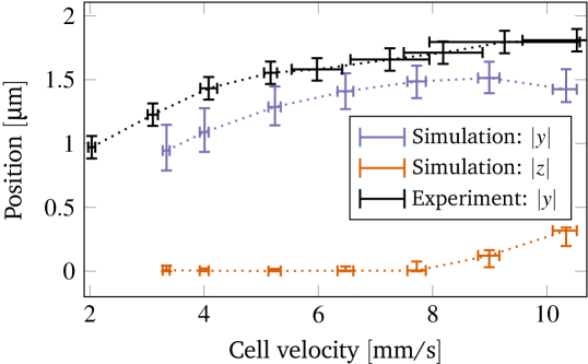
For slippers, the simulations showed an increase of the radial position of up to around (figure 7(a)). Considering the - and -coordinates separately in figure 9, we see that and the major offset happens in the -direction. This is rather fortunate as the -offset is also easily accessible in the experiments, contrary to the -offset. As can be seen in the measured -distribution (figure 3(b)), we have two off-centered peaks for slippers. Taking the distribution function for only the slippers, we extract the positions and of the two peaks. Exploiting the -symmetry of the channel, the off-centered position is then computed as , i.e. in essence as the average of the two peak distances to the central minimum. Figure 9 compares these values with the numerical results: The behavior is the same (an increase with velocity) and the predicted values show only a small systematic deviation of around , i.e. of less than of the RBC diameter . A possible reason is that the optically recorded boundaries of the RBC and the channel walls are somewhat blurry (compare the experimental images in figure 1).
V.4 Implications of the comparison
There has been quite some debate in the literature if the croissant (or parachute) shapes observed via light microscopy are indeed what they appear to be. Gaehtgens et al. (1980) (fig. 4 therein), for example, solidified the flowing RBCs with glutaraldehyde and found that the croissant-like shapes were actually slipper-like. Skalak and Branemark (1969) pointed out that such shapes can also be “edge-on” discocytes with a flattened back. Ultimately, to uniquely identify the forms one needs some method to record the full 3D geometry of the flowing cells (e.g. as in references 32; 91; 92; 93; 94; 15; 26). This is unfortunately very hard to implement in the present experimental setup. However, this missing information is complemented here by the numerical simulations which are in good agreement with the experiments and thus our interpretation of the shapes as croissants should be correct.
The good agreement furthermore implies that our red blood cell model and simulation method is fully appropriate for describing the flow of RBCs in a straight microchannel. More sophisticated methods including e.g. thermal fluctuations or surface viscosity Noguchi and Gompper (2005); McWhirter et al. (2011); Tomaiuolo et al. (2011); Yazdani and Bagchi (2013); Fedosov et al. (2014); Prado et al. (2015) are, at least for the present geometry, not required. For croissants this is intuitive since membrane movement such as tank-treading is absent, for the tank-treading slippers it is somewhat less obvious.
VI Summary & conclusion
To summarize, we have performed in-vitro experiments and 3D simulations of healthy red blood cells flowing in a microchannel. The viscosity ratio was approximately and the flow velocities ranged from around to in both methodologies, corresponding to the typical conditions prevailing in the microvascular system. We found that both the flow velocity as well as the initial starting configuration (offset from channel center, shape) have a major impact on the final steady state of the cells. Using three different starting shapes (discocyte, croissant, slipper), we constructed the corresponding phase diagrams via simulations. In most cases the cells assumed one out of two different forms: either a centered croissant or an off-centered slipper. Interestingly, for most velocities bistability, i.e. a dependence of the final shape on the initial position, was observed. Only in a small range of velocities (at around ) was the final shape found to be always a croissant. The experimental diagram showed very good agreement with the numerical result, especially when considering the simulations that used the rather asymmetric slipper as starting shape.
We thus conclude that the employed numerical RBC model can sensibly describe the cell behavior in the presented setup. Moreover, since we used physiological viscosity ratios and flow velocities, we speculate that croissants and slippers can occur in the microvasculature at the same set of system parameters not just as transients but rather that both are states which are intrinsically assumed by the cells. Our results are important for applications where the cells should be in a specific state (e.g. in lab-on-a-chip devices) and allow for a comprehensive validation of numerical models.
Conflicts of interest
There are no conflicts to declare.
Acknowledgements.
A. Guckenberger and A. Kihm contributed equally to this work. S. Gekle and C. Wagner contributed equally to this work. Funding from the Volkswagen Foundation and computing time granted by the Leibniz-Rechenzentrum on SuperMUC are gratefully acknowledged by A. Guckenberger and S. Gekle. A. Kihm, T. John and C. Wagner kindly acknowledge the support and funding of the “Deutsch-Französische-Hochschule” (DFH) DFDK “Living Fluids”.References
- Freund (2013) J. B. Freund, “The flow of red blood cells through a narrow spleen-like slit,” Phys. Fluids 25, 110807 (2013).
- Picot et al. (2015) J. Picot, P. A. Ndour, S. D. Lefevre, W. El Nemer, H. Tawfik, J. Galimand, L. Da Costa, J.-A. Ribeil, M. de Montalembert, V. Brousse, B. Le Pioufle, P. Buffet, C. Le Van Kim, and O. Français, “A biomimetic microfluidic chip to study the circulation and mechanical retention of red blood cells in the spleen,” Am. J. Hematol. 90, 339 (2015).
- Salehyar and Zhu (2016) S. Salehyar and Q. Zhu, “Deformation and internal stress in a red blood cell as it is driven through a slit by an incoming flow,” Soft Matter 12, 3156 (2016).
- Fedosov et al. (2014) D. A. Fedosov, M. Peltomäki, and G. Gompper, “Deformation and dynamics of red blood cells in flow through cylindrical microchannels,” Soft Matter 10, 4258 (2014).
- Aouane et al. (2014) O. Aouane, M. Thiébaud, A. Benyoussef, C. Wagner, and C. Misbah, “Vesicle dynamics in a confined Poiseuille flow: From steady state to chaos,” Phys. Rev. E 90, 033011 (2014).
- Tahiri et al. (2013) N. Tahiri, T. Biben, H. Ez-Zahraouy, A. Benyoussef, and C. Misbah, “On the problem of slipper shapes of red blood cells in the microvasculature,” Microvasc. Res. 85, 40 (2013).
- Vitkova et al. (2008) V. Vitkova, M.-A. Mader, B. Polack, C. Misbah, and T. Podgorski, “Micro-Macro Link in Rheology of Erythrocyte and Vesicle Suspensions,” Biophys. J. 95, L33 (2008).
- Fedosov et al. (2011) D. A. Fedosov, W. Pan, B. Caswell, G. Gompper, and G. E. Karniadakis, “Predicting human blood viscosity in silico,” Proc. Natl. Acad. Sci. 108, 11772 (2011).
- Krüger et al. (2013) T. Krüger, M. Gross, D. Raabe, and F. Varnik, “Crossover from tumbling to tank-treading-like motion in dense simulated suspensions of red blood cells,” Soft Matter 9, 9008 (2013).
- Thiébaud et al. (2014) M. Thiébaud, Z. Shen, J. Harting, and C. Misbah, “Prediction of Anomalous Blood Viscosity in Confined Shear Flow,” Phys. Rev. Lett. 112, 238304 (2014).
- Katanov et al. (2015) D. Katanov, G. Gompper, and D. A. Fedosov, “Microvascular blood flow resistance: Role of red blood cell migration and dispersion,” Microvasc. Res. 99, 57 (2015).
- Lanotte et al. (2016) L. Lanotte, J. Mauer, S. Mendez, D. A. Fedosov, J.-M. Fromental, V. Claveria, F. Nicoud, G. Gompper, and M. Abkarian, “Red cells’ dynamic morphologies govern blood shear thinning under microcirculatory flow conditions,” Proc. Natl. Acad. Sci. 113, 13289 (2016).
- Henry et al. (2016) E. Henry, S. H. Holm, Z. Zhang, J. P. Beech, J. O. Tegenfeldt, D. A. Fedosov, and G. Gompper, “Sorting cells by their dynamical properties,” Sci. Rep. 6, 34375 (2016).
- Otto et al. (2015) O. Otto, P. Rosendahl, A. Mietke, S. Golfier, C. Herold, D. Klaue, S. Girardo, S. Pagliara, A. Ekpenyong, A. Jacobi, M. Wobus, N. Töpfner, U. F. Keyser, J. Mansfeld, E. Fischer-Friedrich, and J. Guck, “Real-time deformability cytometry: On-the-fly cell mechanical phenotyping,” Nat. Methods 12, 199 (2015).
- Merola et al. (2017) F. Merola, P. Memmolo, L. Miccio, R. Savoia, M. Mugnano, A. Fontana, G. D’Ippolito, A. Sardo, A. Iolascon, A. Gambale, and P. Ferraro, “Tomographic Flow Cytometry by Digital Holography,” Light Sci. Appl. 6, e16241 (2017).
- Farutin and Misbah (2014) A. Farutin and C. Misbah, “Symmetry breaking and cross-streamline migration of three-dimensional vesicles in an axial Poiseuille flow,” Phys. Rev. E 89, 042709 (2014).
- Gaehtgens et al. (1980) P. Gaehtgens, C. Dührssen, and K. H. Albrecht, “Motion, deformation, and interaction of blood cells and plasma during flow through narrow capillary tubes,” Blood Cells 6, 799 (1980).
- Suzuki et al. (1996) Y. Suzuki, N. Tateishi, M. Soutani, and N. Maeda, “Deformation of Erythrocytes in Microvessels and Glass Capillaries: Effects of Erythrocyte Deformability,” Microcirculation 3, 49 (1996).
- Secomb et al. (2007) T. W. Secomb, B. Styp-Rekowska, and A. R. Pries, “Two-Dimensional Simulation of Red Blood Cell Deformation and Lateral Migration in Microvessels,” Ann. Biomed. Eng. 35, 755 (2007).
- Faivre (2006) M. Faivre, Drops, Vesicles and Red Blood Cells: Deformability and Behavior under Flow, Ph.D. thesis, Université Joseph-Fourier - Grenoble I, Grenoble (2006).
- Abkarian et al. (2008) M. Abkarian, M. Faivre, R. Horton, K. Smistrup, C. A. Best-Popescu, and H. A. Stone, “Cellular-scale hydrodynamics,” Biomed. Mater. 3, 034011 (2008).
- Tomaiuolo et al. (2009) G. Tomaiuolo, M. Simeone, V. Martinelli, B. Rotoli, and S. Guido, “Red blood cell deformation in microconfined flow,” Soft Matter 5, 3736 (2009).
- Tomaiuolo and Guido (2011) G. Tomaiuolo and S. Guido, “Start-up shape dynamics of red blood cells in microcapillary flow,” Microvasc. Res. 82, 35 (2011).
- Prado et al. (2015) G. Prado, A. Farutin, C. Misbah, and L. Bureau, “Viscoelastic Transient of Confined Red Blood Cells,” Biophys. J. 108, 2126 (2015).
- Cluitmans et al. (2014) J. C. A. Cluitmans, V. Chokkalingam, A. M. Janssen, R. Brock, W. T. S. Huck, and G. J. C. G. M. Bosman, “Alterations in Red Blood Cell Deformability during Storage: A Microfluidic Approach,” BioMed Res. Int. 2014, e764268 (2014).
- Quint et al. (2017) S. Quint, A. F. Christ, A. Guckenberger, S. Himbert, L. Kaestner, S. Gekle, and C. Wagner, “3D tomography of cells in micro-channels,” Appl. Phys. Lett. 111, 103701 (2017).
- Hochmuth et al. (1970) R. M. Hochmuth, R. N. Marple, and S. P. Sutera, “Capillary blood flow: I. Erythrocyte deformation in glass capillaries,” Microvascular Research 2, 409 (1970).
- Seshadri et al. (1970) V. Seshadri, R. M. Hochmuth, P. A. Croce, and S. P. Sutera, “Capillary blood flow: III. Deformable model cells compared to erythrocytes in vitro,” Microvascular Research 2, 434 (1970).
- Zharov et al. (2006) V. P. Zharov, E. I. Galanzha, Y. Menyaev, and V. V. Tuchin, “In vivo high-speed imaging of individual cells in fast blood flow,” J. Biomed. Opt 11, 054034 (2006).
- Tomaiuolo et al. (2007) G. Tomaiuolo, V. Preziosi, M. Simeone, S. Guido, R. Ciancia, V. Martinelli, C. Rinaldi, and B. Rotoli, “A methodology to study the deformability of red blood cells flowing in microcapillaries in vitro,” Ann. Ist. Super. Sanità 43, 186 (2007).
- Guido and Tomaiuolo (2009) S. Guido and G. Tomaiuolo, “Microconfined flow behavior of red blood cells in vitro,” Comptes Rendus Phys. 10, 751 (2009).
- Gorthi and Schonbrun (2012) S. S. Gorthi and E. Schonbrun, “Phase imaging flow cytometry using a focus-stack collecting microscope,” Opt. Lett. 37, 707 (2012).
- Lanotte et al. (2014) L. Lanotte, G. Tomaiuolo, C. Misbah, L. Bureau, and S. Guido, “Red blood cell dynamics in polymer brush-coated microcapillaries: A model of endothelial glycocalyx in vitro,” Biomicrofluidics 8, 014104 (2014).
- Tomaiuolo et al. (2016) G. Tomaiuolo, L. Lanotte, R. D’Apolito, A. Cassinese, and S. Guido, “Microconfined flow behavior of red blood cells,” Med. Eng. Phys. 38, 11 (2016).
- Claver´ıa et al. (2016) V. Clavería, O. Aouane, M. Thiébaud, M. Abkarian, G. Coupier, C. Misbah, T. John, and C. Wagner, “Clusters of red blood cells in microcapillary flow: Hydrodynamic versus macromolecule induced interaction,” Soft Matter 12, 8235 (2016).
- Guest et al. (1963) M. M. Guest, T. P. Bond, R. G. Cooper, and J. R. Derrick, “Red Blood Cells: Change in Shape in Capillaries,” Science 142, 1319 (1963).
- Skalak and Branemark (1969) R. Skalak and P. I. Branemark, “Deformation of Red Blood Cells in Capillaries,” Science 164, 717 (1969).
- Kubota et al. (1996) K. Kubota, J. Tamura, T. Shirakura, M. K Imura, K. Y Amanaka, T. Isozaki, and I. Nishio, “The behaviour of red cells in narrow tubes in vitro as a model of the microcirculation,” Br. J. Haematol. 94, 266 (1996).
- Tomaiuolo et al. (2012) G. Tomaiuolo, L. Lanotte, G. Ghigliotti, C. Misbah, and S. Guido, “Red blood cell clustering in Poiseuille microcapillary flow,” Phys. Fluids 24, 051903 (2012).
- Wagner et al. (2013) C. Wagner, P. Steffen, and S. Svetina, “Aggregation of red blood cells: From rouleaux to clot formation,” Comptes Rendus Physique Living fluids / Fluides vivants, 14, 459 (2013).
- Brust et al. (2014) M. Brust, O. Aouane, M. Thiébaud, D. Flormann, C. Verdier, L. Kaestner, M. W. Laschke, H. Selmi, A. Benyoussef, T. Podgorski, G. Coupier, C. Misbah, and C. Wagner, “The plasma protein fibrinogen stabilizes clusters of red blood cells in microcapillary flows,” Sci. Rep. 4, 4348 (2014).
- Goldsmith and Marlow (1972) H. L. Goldsmith and J. Marlow, “Flow Behaviour of Erythrocytes. I. Rotation and Deformation in Dilute Suspensions,” Proc. R. Soc. Lond. B Biol. Sci. 182, 351 (1972).
- Secomb et al. (1986) T. W. Secomb, R. Skalak, N. Özkaya, and J. F. Gross, “Flow of axisymmetric red blood cells in narrow capillaries,” J. Fluid Mech. 163, 405 (1986).
- Secomb (1987) T. W. Secomb, “Flow-dependent rheological properties of blood in capillaries,” Microvascular Research 34, 46 (1987).
- Secomb et al. (2001) T. W. Secomb, R. Hsu, and A. R. Pries, “Motion of red blood cells in a capillary with an endothelial surface layer: Effect of flow velocity,” Am. J. Physiol. - Heart Circ. Physiol. 281, H629 (2001).
- Secomb and Skalak (1982) T. W. Secomb and R. Skalak, “A two-dimensional model for capillary flow of an asymmetric cell,” Microvascular Research 24, 194 (1982).
- Kaoui et al. (2009a) B. Kaoui, G. Biros, and C. Misbah, “Why Do Red Blood Cells Have Asymmetric Shapes Even in a Symmetric Flow?” Phys. Rev. Lett. 103, 188101 (2009a).
- Kaoui et al. (2011) B. Kaoui, N. Tahiri, T. Biben, H. Ez-Zahraouy, A. Benyoussef, G. Biros, and C. Misbah, “Complexity of vesicle microcirculation,” Phys. Rev. E 84, 041906 (2011).
- Kaoui et al. (2012) B. Kaoui, T. Krüger, and J. Harting, “How does confinement affect the dynamics of viscous vesicles and red blood cells?” Soft Matter 8, 9246 (2012).
- Shi et al. (2012) L. Shi, T.-W. Pan, and R. Glowinski, “Deformation of a single red blood cell in bounded Poiseuille flows,” Phys. Rev. E 85, 016307 (2012), 10.1103/PhysRevE.85.016307.
- Lázaro et al. (2014) G. R. Lázaro, A. Hernández-Machado, and I. Pagonabarraga, “Rheology of red blood cells under flow in highly confined microchannels: I. effect of elasticity,” Soft Matter 10, 7195 (2014).
- Noguchi and Gompper (2005) H. Noguchi and G. Gompper, “Shape transitions of fluid vesicles and red blood cells in capillary flows,” Proc. Natl. Acad. Sci. 102, 14159 (2005).
- McWhirter et al. (2011) J. L. McWhirter, H. Noguchi, and G. Gompper, “Deformation and clustering of red blood cells in microcapillary flows,” Soft Matter 7, 10967 (2011).
- Ye et al. (2017) T. Ye, H. Shi, L. Peng, and Y. Li, “Numerical studies of a red blood cell in rectangular microchannels,” J. Appl. Phys. 122, 084701 (2017).
- Kaoui et al. (2009b) B. Kaoui, G. Coupier, C. Misbah, and T. Podgorski, “Lateral migration of vesicles in microchannels: Effects of walls and shear gradient,” Houille Blanche , 112 (2009b).
- Cordasco et al. (2014) D. Cordasco, A. Yazdani, and P. Bagchi, “Comparison of erythrocyte dynamics in shear flow under different stress-free configurations,” Phys. Fluids 26, 041902 (2014).
- Peng et al. (2014) Z. Peng, A. Mashayekh, and Q. Zhu, “Erythrocyte responses in low-shear-rate flows: Effects of non-biconcave stress-free state in the cytoskeleton,” J. Fluid Mech. 742, 96 (2014).
- Sinha and Graham (2015) K. Sinha and M. D. Graham, “Dynamics of a single red blood cell in simple shear flow,” Phys. Rev. E 92, 042710 (2015).
- Cokelet and Meiselman (1968) G. R. Cokelet and H. J. Meiselman, “Rheological Comparison of Hemoglobin Solutions and Erythrocyte Suspensions,” Science 162, 275 (1968).
- Popel and Johnson (2005) A. S. Popel and P. C. Johnson, “Microcirculation and Hemorheology,” Annu. Rev. Fluid Mech. 37, 43 (2005).
- Cui et al. (2002) B. Cui, H. Diamant, and B. Lin, “Screened Hydrodynamic Interaction in a Narrow Channel,” Phys. Rev. Lett. 89, 188302 (2002).
- Diamant (2009) H. Diamant, “Hydrodynamic Interaction in Confined Geometries,” J. Phys. Soc. Jpn. 78, 041002 (2009).
- Koller et al. (1987) A. Koller, B. Dawant, A. Liu, A. S. Popel, and P. C. Johnson, “Quantitative analysis of arteriolar network architecture in cat sartorius muscle,” Am. J. Physiol. - Heart Circ. Physiol. 253, H154 (1987).
- Evans and Fung (1972) E. Evans and Y.-C. Fung, “Improved measurements of the erythrocyte geometry,” Microvasc. Res. 4, 335 (1972).
- Le (2010) D.-V. Le, “Subdivision elements for large deformation of liquid capsules enclosed by thin shells,” Comput. Methods Appl. Mech. Eng. 199, 2622 (2010).
- Chien et al. (1966) S. Chien, S. Usami, H. M. Taylor, J. L. Lundberg, and M. I. Gregersen, “Effects of hematocrit and plasma proteins on human blood rheology at low shear rates.” J. Appl. Physiol. 21, 81 (1966).
- Skalak et al. (1989) R. Skalak, N. Ozkaya, and T. C. Skalak, “Biofluid Mechanics,” Annu. Rev. Fluid Mech. 21, 167 (1989).
- Secomb (2017) T. W. Secomb, “Blood Flow in the Microcirculation,” Annu. Rev. Fluid Mech. 49, 443 (2017).
- Kim et al. (2014) Y. Kim, H. Shim, K. Kim, H. Park, S. Jang, and Y. Park, “Profiling individual human red blood cells using common-path diffraction optical tomography,” Sci. Rep. 4, 6659 (2014).
- Skalak et al. (1973) R. Skalak, A. Tozeren, R. P. Zarda, and S. Chien, “Strain Energy Function of Red Blood Cell Membranes,” Biophys. J. 13, 245 (1973).
- Krüger et al. (2011) T. Krüger, F. Varnik, and D. Raabe, “Efficient and accurate simulations of deformable particles immersed in a fluid using a combined immersed boundary lattice Boltzmann finite element method,” Comput. Math. Appl. 61, 3485 (2011).
- Yoon et al. (2008) Y.-Z. Yoon, J. Kotar, G. Yoon, and P. Cicuta, “The nonlinear mechanical response of the red blood cell,” Phys. Biol. 5, 036007 (2008).
- Freund (2014) J. B. Freund, “Numerical Simulation of Flowing Blood Cells,” Annu. Rev. Fluid Mech. 46, 67 (2014).
- Canham (1970) P. B. Canham, “The minimum energy of bending as a possible explanation of the biconcave shape of the human red blood cell,” J. Theor. Biol. 26, 61 (1970).
- Helfrich (1973) W. Helfrich, “Elastic Properties of Lipid Bilayers: Theory and Possible Experiments,” Z. Naturforsch. C 28, 693 (1973).
- Guckenberger and Gekle (2017a) A. Guckenberger and S. Gekle, “Theory and algorithms to compute Helfrich bending forces: A review,” J. Phys. Condens. Matter 29, 203001 (2017a).
- Park et al. (2010) Y. Park, C. A. Best, K. Badizadegan, R. R. Dasari, M. S. Feld, T. Kuriabova, M. L. Henle, A. J. Levine, and G. Popescu, “Measurement of red blood cell mechanics during morphological changes,” Proc. Natl. Acad. Sci. 107, 6731 (2010).
- Guckenberger et al. (2016) A. Guckenberger, M. P. Schraml, P. G. Chen, M. Leonetti, and S. Gekle, “On the bending algorithms for soft objects in flows,” Comput. Phys. Comm. 207, 1 (2016).
- Farutin et al. (2014) A. Farutin, T. Biben, and C. Misbah, “3D numerical simulations of vesicle and inextensible capsule dynamics,” J. Comput. Phys. 275, 539 (2014).
- Guckenberger and Gekle (2017b) A. Guckenberger and S. Gekle, “A boundary integral method with volume-changing objects for ultrasound-triggered margination of microbubbles,” arXiv:1608.05196 [physics] (2017b), arXiv:1608.05196 [physics] .
- Pozrikidis (2001) C. Pozrikidis, “Interfacial Dynamics for Stokes Flow,” J. Comput. Phys. 169, 250 (2001).
- Zhao et al. (2010) H. Zhao, A. H. Isfahani, L. N. Olson, and J. B. Freund, “A spectral boundary integral method for flowing blood cells,” J. Comput. Phys. 229, 3726 (2010).
- Saintillan et al. (2005) D. Saintillan, E. Darve, and E. S. G. Shaqfeh, “A smooth particle-mesh Ewald algorithm for Stokes suspension simulations: The sedimentation of fibers,” Phys. Fluids 17, 033301 (2005).
- Saad and Schultz (1986) Y. Saad and M. Schultz, “GMRES: A Generalized Minimal Residual Algorithm for Solving Nonsymmetric Linear Systems,” SIAM J. Sci. Stat. Comput. 7, 856 (1986).
- Bogacki and Shampine (1989) P. Bogacki and L. F. Shampine, “A 3(2) pair of Runge - Kutta formulas,” Appl. Math. Lett. 2, 321 (1989).
- Daddi-Moussa-Ider et al. (2016) A. Daddi-Moussa-Ider, A. Guckenberger, and S. Gekle, “Long-lived anomalous thermal diffusion induced by elastic cell membranes on nearby particles,” Phys. Rev. E 93, 012612 (2016).
- Pries et al. (1995) A. R. Pries, T. W. Secomb, and P. Gaehtgens, “Structure and hemodynamics of microvascular networks: Heterogeneity and correlations,” Am. J. Physiol. - Heart Circ. Physiol. 269, H1713 (1995).
- Baskurt et al. (2011) O. Baskurt, B. Neu, and H. Meiselman, Red Blood Cell Aggregation (CRC Press, 2011).
- Kaoui and Harting (2016) B. Kaoui and J. Harting, “Two-dimensional lattice Boltzmann simulations of vesicles with viscosity contrast,” Rheol Acta 55, 465 (2016).
- Schaaf and Stark (2017) C. Schaaf and H. Stark, “Inertial migration and axial control of deformable capsules,” Soft Matter 13, 3544 (2017).
- Pégard and Fleischer (2013) N. C. Pégard and J. W. Fleischer, “Three-dimensional deconvolution microfluidic microscopy using a tilted channel,” J. Biomed. Opt. 18, 040503 (2013).
- Pégard et al. (2014) N. C. Pégard, M. L. Toth, M. Driscoll, and J. W. Fleischer, “Flow-scanning optical tomography,” Lab Chip 14, 4447 (2014).
- Jagannadh et al. (2016) V. K. Jagannadh, M. D. Mackenzie, P. Pal, A. K. Kar, and S. S. Gorthi, “Slanted channel microfluidic chip for 3D fluorescence imaging of cells in flow,” Opt. Express 24, 22144 (2016).
- Kim et al. (2016) K. Kim, K. Choe, I. Park, P. Kim, and Y. Park, “Holographic intravital microscopy for 2-D and 3-D imaging intact circulating blood cells in microcapillaries of live mice,” Sci. Rep. 6, 33084 (2016).
- Tomaiuolo et al. (2011) G. Tomaiuolo, M. Barra, V. Preziosi, A. Cassinese, B. Rotoli, and S. Guido, “Microfluidics analysis of red blood cell membrane viscoelasticity,” Lab Chip 11, 449 (2011).
- Yazdani and Bagchi (2013) A. Yazdani and P. Bagchi, “Influence of membrane viscosity on capsule dynamics in shear flow,” J. Fluid Mech. 718, 569 (2013).
See pages 1 of SI.pdf
See pages 2 of SI.pdf
See pages 3 of SI.pdf
See pages 4 of SI.pdf
See pages 5 of SI.pdf
See pages 6 of SI.pdf
See pages 7 of SI.pdf
See pages 8 of SI.pdf
See pages 9 of SI.pdf
See pages 10 of SI.pdf
See pages 11 of SI.pdf
See pages 12 of SI.pdf
See pages 13 of SI.pdf