Numerical Simulation of Current Sheet Formation in a Quasi-Separatrix Layer using Adaptive Mesh Refinement
Abstract
The formation of a thin current sheet in a magnetic quasi-separatrix layer (QSL) is investigated by means of numerical simulation using a simplified ideal, low-, MHD model. The initial configuration and driving boundary conditions are relevant to phenomena observed in the solar corona and were studied earlier by Aulanier et al., A&A 444, 961 (2005). In extension to that work, we use the technique of adaptive mesh refinement (AMR) to significantly enhance the local spatial resolution of the current sheet during its formation, which enables us to follow the evolution into a later stage. Our simulations are in good agreement with the results of Aulanier et al. up to the calculated time in that work. In a later phase, we observe a basically unarrested collapse of the sheet to length scales that are more than one order of magnitude smaller than those reported earlier. The current density attains correspondingly larger maximum values within the sheet. During this thinning process, which is finally limited by lack of resolution even in the AMR studies, the current sheet moves upward, following a global expansion of the magnetic structure during the quasi-static evolution. The sheet is locally one-dimensional and the plasma flow in its vicinity, when transformed into a co-moving frame, qualitatively resembles a stagnation point flow. In conclusion, our simulations support the idea that extremely high current densities are generated in the vicinities of QSLs as a response to external perturbations, with no sign of saturation.
I Introduction
The spontaneous formation of thin current sheets is believed to play an important role in the dynamics of astrophysical plasmas like the solar corona and, in particular, for the onset of magnetic reconnection. In fact, impulsive events like solar flares and coronal mass ejections are often associated with magnetic reconnection as a mechanism that effectively releases magnetic energy, which in turn calls for highly concentrated electrical currents to explain the breakdown of ideal plasma behavior by means of e.g. micro-instabilities in the non-collisional coronal plasma.
Recently, the study of magnetic field configurations as candidates for reconnection has shifted from separatrix surfaces towards quasi-separatrix layers (QSLs) Démoulin et al. (1996a, b); Milano et al. (1999). In contrast to genuine separatrix configurations, QSL fields do not necessarily contain magnetic null points in 3D, which makes them relevant in many more situations than strict separatrices. QSLs describe a magnetic field mapping between two boundaries that is continuous, but changes rapidly in space. This change has been quantified in terms of a flux tube “squashing factor” Titov and Hornig (2002) and more recently generalized to remove boundary projection effects Titov (2007). In accordance with the significance of QSLs for magnetic reconnection, the problem of current sheet formation has been investigated. Here, Titov et al. Titov et al. (2003) and Galsgaard et al. Galsgaard et al. (2003) studied the formation of current sheets in a straight hyperbolic flux tube (HFT) configuration both analytically and numerically, and found exponential growth of the current density as a response to shearing magnetic footpoint motion. One major conclusion of that work was that a shear in the applied boundary motion was important, if not essential, for the formation of thin current sheets, and that the creation of a stagnation point flow in the HFT was the key element in this process. However, this has been later questioned by Aulanier et al. Aulanier et al. (2005): They argued that the initial squashing factor in the simulations of Galsgaard et al., probably together with additional symmetry properties, was too small to account for highly concentrated currents, and that the shear boundary motion and stagnation point flow in Galsgaard et al. (2003) served as to dynamically create thin QSLs only during the simulation. This argument was underpinned in Aulanier et al. (2005) through extensive comparison between MHD simulations of less symmetric potential magnetic field configurations which initially result from four magnetic point sources submerged below a photospheric boundary. They contain QSLs with squashing factors of up to and were exposed to different boundary driver patterns, namely a shear and a translational motion. Aulanier et al. observed the formation of thin, intense current sheets, almost irrespective of the type of applied boundary driving, which stresses the relevance of the initial field geometry and QSL strength, rather than the boundary motion, for current sheet formation. Later, that work has been extended by finite resistivity to simulate magnetic reconnection at that thin current sheet Aulanier et al. (2006) with its strong temporal change in magnetic connectivity.
A general limitation of these previous numerical studies was the lack of reasonable numerical grid resolution at the sites of current sheet formation Aulanier et al. (2006): During the formation process, the currents get more and more concentrated locally so that the sheet scales quickly reach the numerical grid spacing. This left open the question whether the current concentration would continue to length scales small enough to account for the onset of micro-instabilities, or if this process would get arrested at some larger length scale. In order to address this question, but also get more insight into the local dynamics in the immediate vicinities of the current sheets, we have carried out numerical simulations in the spirit of Aulanier et al. (2005), using one of their initial configurations and boundary drivers. However, we used the technique of adaptive mesh refinement (AMR), implemented in the code racoon Dreher and Grauer (2005), in order to obtain a much higher grid resolution in the current sheet vicinity than was reported earlier. This allowed us to obtain insight into the formation process that reaches beyond the previous results.
In the next section, we will briefly describe the model that we employed in our studies, while results that complement the work of Aulanier et al. (2005) are given in Sec. III, followed by a summary and conclusion in the last section.
II Basic equations and numerical model
Our simulations are based on a reduced subset of the MHD equations, appropriate for the quasi-static, low- regime, where is the ratio of thermal to magnetic pressure. In normalized quantities, it reads
| (1a) | |||||
| (1b) | |||||
| (1c) | |||||
| (1d) | |||||
Pressure terms are omitted from the momentum equation (1a) because of the low- approximation. As we are interested in a quasi-stationary evolution of the system, i.e. the limit of high wave speeds, we replace the continuity equation by a direct prescription of a relaxation mass density, namely . This approach results in an homogeneous Alfvén velocity and fast communication of unbalanced forces throughout the system, which shortens relaxation times and has been successfully used in other studies Arnold et al. (2008). Constant kinematic viscosity and resistivity are included only to guarantee numerical stability on the grid scale and have little effect on the overall evolution. The artificial scalar function and its dynamic equation (1d) serve as a convenient means to constrain any finite , resulting from discretization errors, to negligible values Dedner et al. (2002): Combining and results in the mixed equation
for . The crucial term on the right side is the first Laplacian, which describes a hyperbolic transport of with velocity and leads to radiative distribution of throughout the computational domain, while it gets dissipated by phase mixing and diffusion according to the other two terms. Note that there is freedom in a specific choice for the -equation (1d) as it is of the order of the discretization error anyway. For instance, while Dedner et al. Dedner et al. (2002) discuss the term (see their Eq. (19) resp. (24e)) to arrive at a telegraph equation for and in the continuous case, we found this unnecessary, although possible, for our computations. The main reason for this seems to be that in our case, the sources of -errors are highly localized regions in space, namely the regions of intense currents, so that the hyperbolic transport is the dominating cleaning effect. On the other hand, we added the term in Eq. (1d), which is not discussed in this specific form in Dedner et al. (2002). Its motivation is, however, not so much a change in the -cleaning property itself, but the observation that the purely hyperbolic choice, i.e. Eq. (1d) with , tends to introduce odd-even-decoupling on the centered finite difference grid that we used. This decoupling, which was not an issue in Dedner et al. (2002) since they employed finite volume schemes in finite element discretisations, could be healed satisfactorily through the additional Laplacian term which couples -values on neighboring grid points with each other. We finally found overall good -cleaning properties when choosing the numerical parameter values to and .
The equations are discretized in a domain of , where we identify the plane with the solar photosphere. Integration is performed with a strongly stable third-order Runge-Kutta scheme Shu and Osher (1988), spatial differentiation is realized with standard second-order finite differences. In order to resolve the expected small-scale features, we employed the block-structured adaptive mesh refinement (AMR) framework racoon Dreher and Grauer (2005). Here, we used the norm of the magnetic field gradient, , to derive a local length scale for that serves as an indicator criterion for local mesh refinement. Effective local grid resolutions obtained with this technique were in the present work.
Initial conditions are adapted from Aulanier et al. (2005), where we address the magnetic field configuration resulting from two pairs of opposite polarity photospheric flux patches whose respective connecting axes intersect at an angle of 150 degrees. Specifically, the initial magnetic field stems from 4 virtual magnetic point sources, indexed by , below the photosphere
| (2) |
with respective source strengths and and locations and , respectively. This field geometry is known to contain two symmetric dome-shaped QSLs with squashing factors of , intersecting in a hyperbolic flux tube (see Aulanier et al. (2005) for details).
In the course of the simulation, the field is exposed to a horizontal photospheric vortex flow around the magnetic source in Eq. (2), realized by prescribing the boundary condition for at . The maximum flow velocity is and it gets ramped up in time according to .
The detailed treatment of the lower boundary is as follows: As all quantities are discretized as cell-centered variables, boundary conditions have to provide values for , and at in a way that is consistent with the evolution equations and the overall second order accuracy in the grid spacing . Denoting the boundary values of individual quantities at with a hat, the velocity is explicitly given from the prescribed horizontal vortex flow, and in particular, . All components of at can now simply be interpolated in -direction with second order accuracy between and the interior grid points above . Using this direct forcing, there is no need to compute or the Lorentz force at at all, hence we do not need the horizontal components of at this stage. Now, to integrate , we note that the convective part of the -equation becomes autonomous in the boundary plane, involving no other undetermined quantities nor any derivatives normal to the boundary: Writing the convective electric field as gives and so that where the index indicates horizontal vector projections, e.g. the prescribed , and . In other words, when ignoring the numerically motivated resistive diffusion and -terms, we are able to integrate the “proper” completely for its own, which in turn allows us again to interpolate at up to , similar to above. Now, this “proper” -equation also determines , which allows to update at . At this point, the magnetic diffusion and -cleaning terms are taken into account as usual, where the former requires an extrapolation of across . Finally, the right side of Eq. (1d) is easily evaluated at , using from above and the Dirichlet condition .
While the upper and lateral boundaries can in principle be handled in the same fashion, using the no-slip and no-penetration condition , we used a simpler approach there: Setting to zero ahead of the boundaries, keeping the tangential components of fixed in ghost cells and applying solenoidal and homogeneous Dirichlet conditions to the normal components of and , respectively, proved to be sufficient for those passive boundaries. Note, in particular, that no artificial Lorentz forces act there either.
The boundary treatment described above presumes a homogeneous numerical grid. It has been applied in the same spirit to the AMR simulations that we present here, where additional complications occur at the interfaces between neighboring grid blocks of different mesh resolution that abut the physical boundaries. Without going into details, we only mention that additional coarse-fine and fine-coarse interpolations are needed for the computation of and at those junctions, but that they do not pose any fundamental new challenge apart from the programming complexity.
III Results
After applying the photospheric boundary driving in , dynamic shear modes travel into the domain and mix there. On the scale of a few Alfvén transit times, the magnitude of the current density grows significantly and a quasi-stationary current system as shown in Fig. 1 builds up.
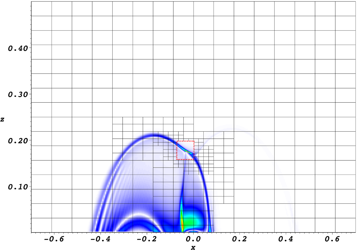
It consists partly of relatively weak currents which are distributed on a large scale in a dome-like structure that is pre-determined by magnetic field lines connecting the driver region with the opposite polarity regions of the photosphere. On top of this, a highly localized thin current sheet can be identified in the vicinity of in Fig. 1. This thin current sheet actually lies inside the pre-existing QSL of the initial magnetic field. We interpret the striation patterns at in Fig. 1 as signatures of MHD waves on field lines which connect the strong photospheric field region with the current sheet during the evolution.
These results are basically in good agreement with those published earlier by Aulanier et al. Aulanier et al. (2005). However, the sheet thickness at the stage shown in Fig. 1 is already on the numerical grid scale of Aulanier et al. (2005), so that their studies were unable to investigate into the further evolution or features on smaller scales.

The temporal evolution of the sheet is displayed in Fig. 2 which shows the vertical profiles of at for four different times. It is evident that the sheet thickness decreases with time while the value of maximum current density increases accordingly to reach values of in the latest stage. At the same time, the sheet moves upwards, as indicated by the inset graphs. In fact, we find that the entire magnetic structure expands gradually as a response to the boundary driving, and the current sheet as a substructure is embedded in this motion. An other detail that emerges from Fig. 2 is the fact that up to , the most intense currents are not yet found in the thin current sheet itself, but in the large-scale system at , i.e. close to the photospheric driver (see also Fig. 1). It is only at later times, that the thin sheet dominates in the current intensity.
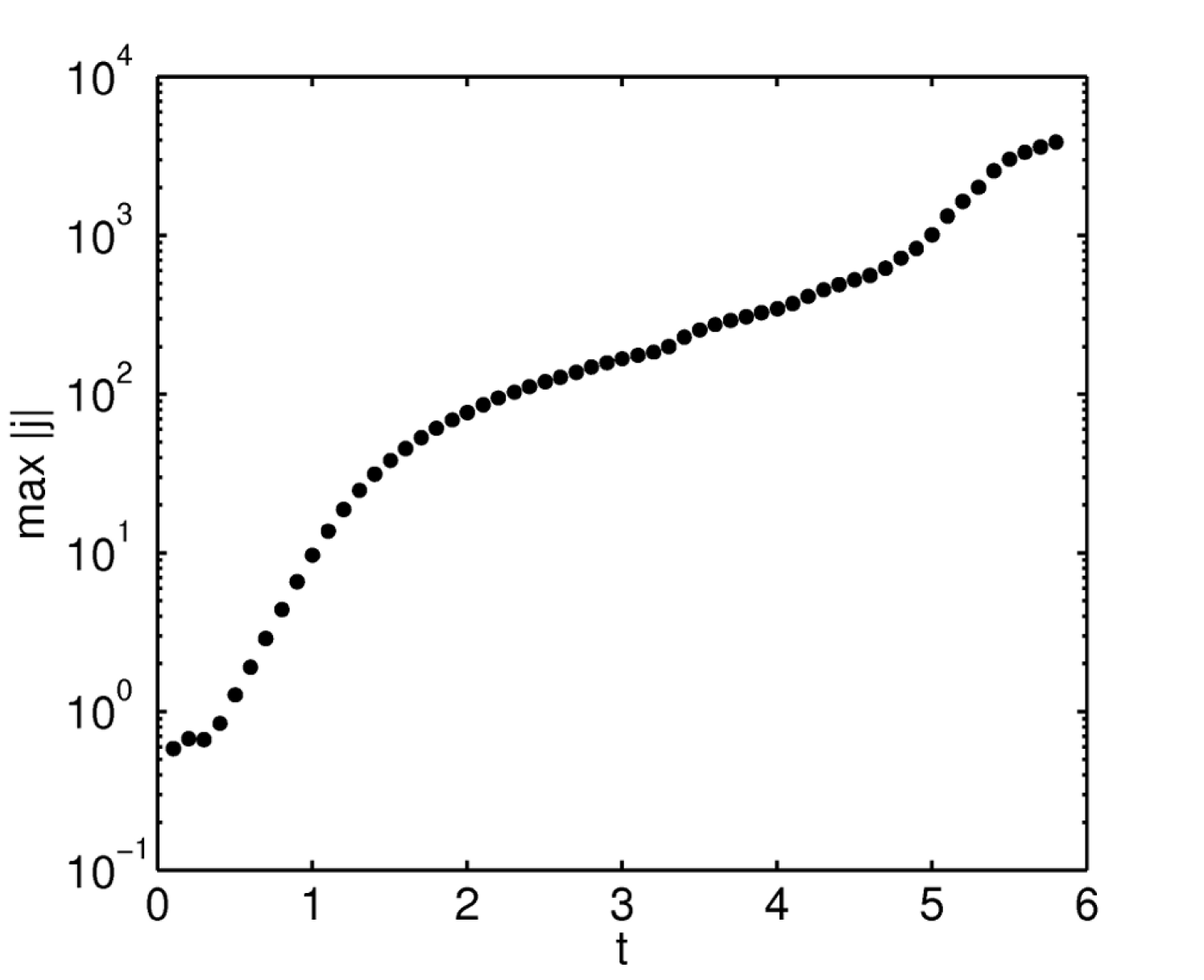
This phenomenon is also visible in the temporal evolution of , which is plotted logarithmically against time in Fig. 3: The early phase, with rather fast growth of , corresponds to the ramp-up of the boundary driver, which essentially reaches its maximum magnitude around . This is followed by a slower growth rate of the current maximum up to . During this stage, the maximum values stem from the extended currents close to the photosphere (compare with Fig. 2), which eventually get overtaken by the faster growth of the thin embedded current sheet. Further intensification continues, with amplification of by roughly a factor of 5, until the growth slows down at . At this time, the sheet thickness is only a few times the numerical grid scale and thereby poorly resolved with artificial diffusion effects becoming competitive.
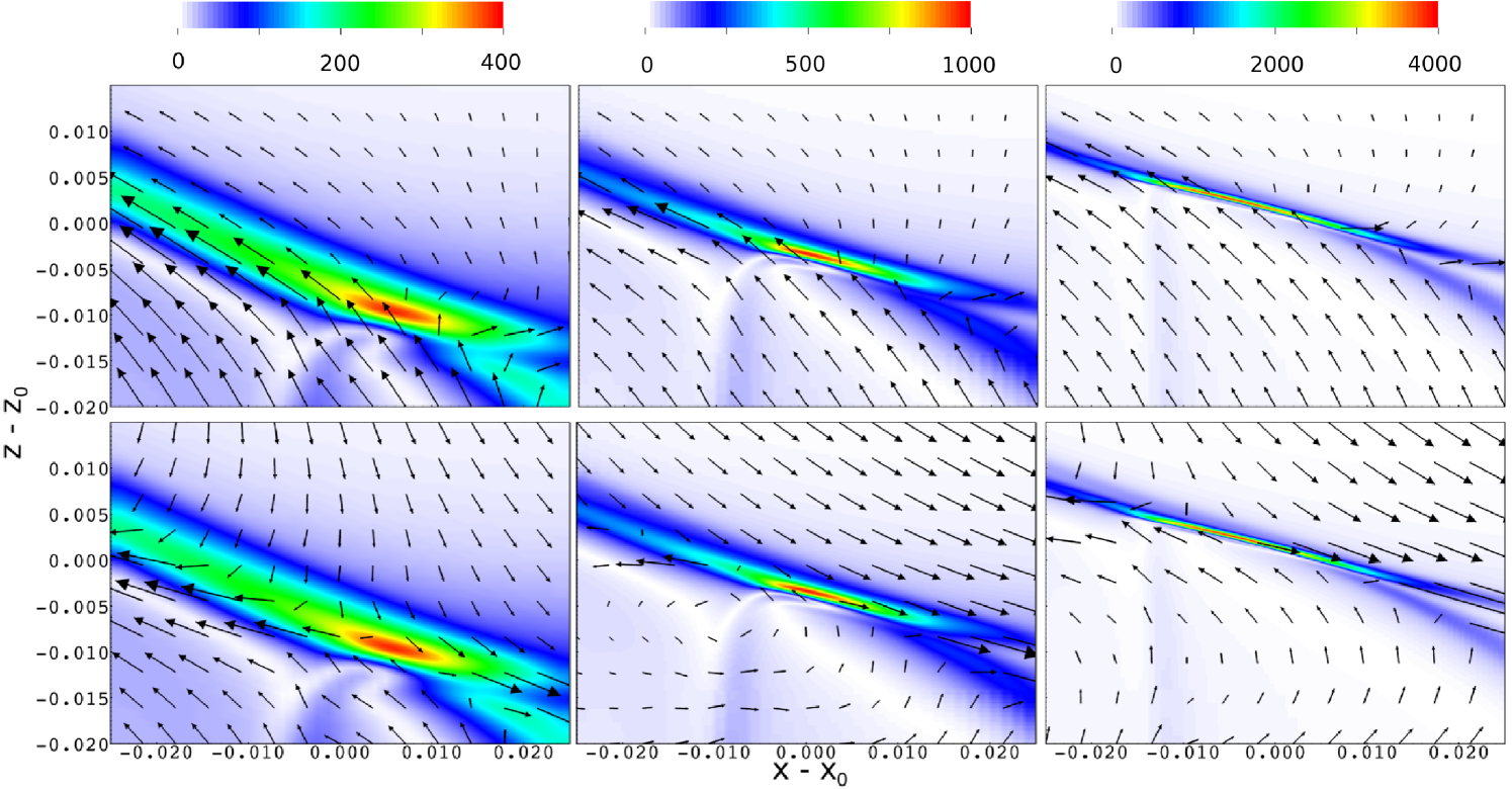
Fig. 4 shows details of the sheet in the cut plane for three different times. Again, the overall upward motion and the thinning and intensification of the sheet are well visible. In addition, we have plotted the plasma velocity as arrows, projected into the displayed plane, to give an impression of the flow in the vicinity of the current sheet. While the upper row shows the velocity relative to the fixed simulation frame, the plots in the lower row show the flow transformed to a frame which is co-moving with the expansion velocity of the structure. To this end, we identified the locations of maximum current density in the plane from plots of successive data output sets, and computed a pattern velocity from their difference. This velocity was then subtracted from the plasma flow velocity in the lower plots of Fig. 4. There have been controversial discussions as to whether the current sheet formation at the hyperbolic flux tube embedded in the QSL is related to a stagnation-point flow Galsgaard et al. (2003); Aulanier et al. (2005). In particular, Aulanier et al. claim that no stagnation point exists at the intense current sheet. This is certainly confirmed by our simulation, however we remark that the focus on a strict definition of stagnation point, i.e. , maybe somewhat misleading because i) the velocity is sensitive to the chosen frame of reference, and ii) the component along the current sheet should be discarded from these considerations anyway, because it largely decouples from the mechanism of magnetic shearing discussed in Titov et al. (2003) and Galsgaard et al. (2003).
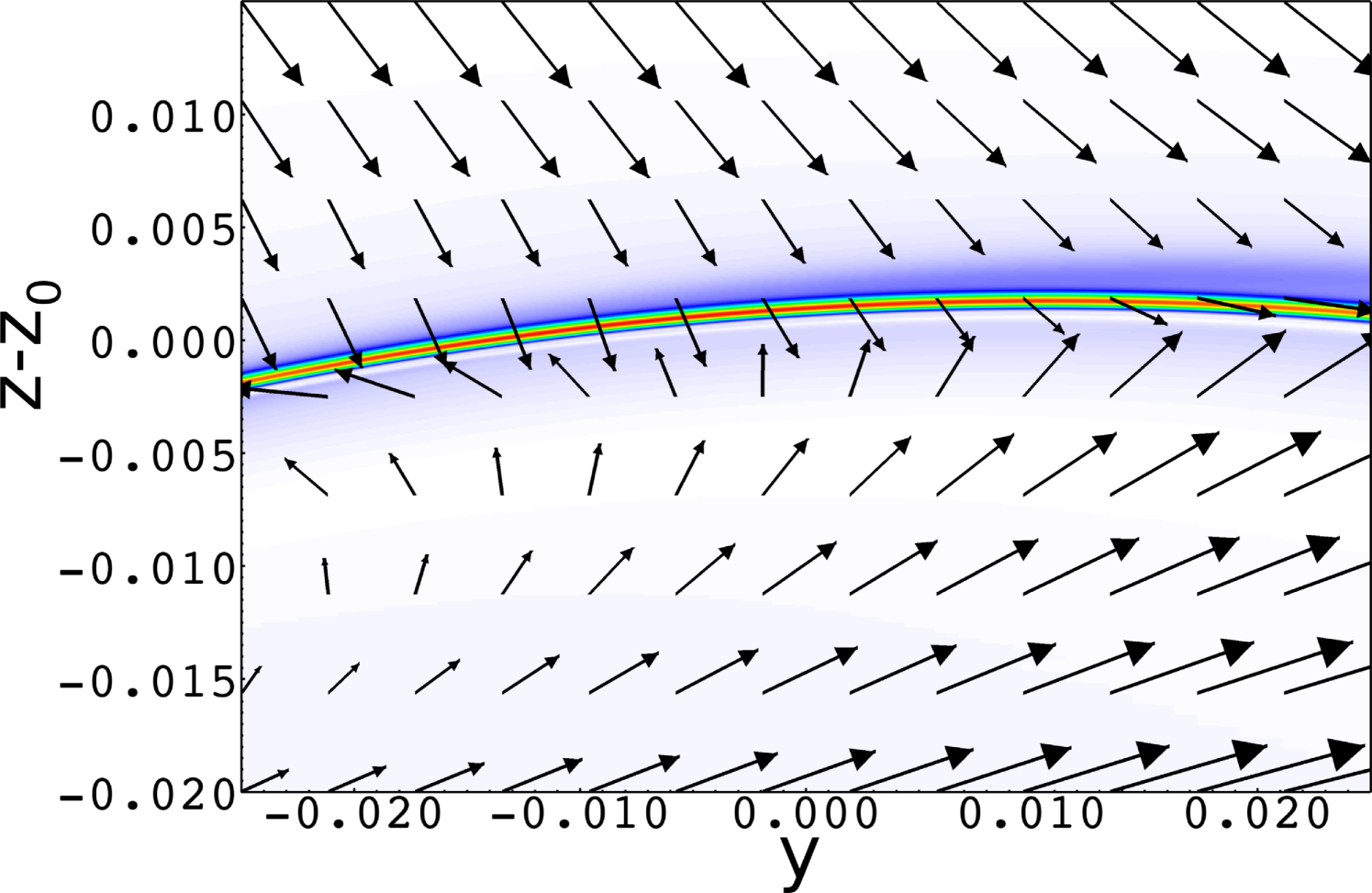
The flow pattern projected into the --plane is shown in Fig. 5, again transformed into a frame that moves upward with the current sheet and, in addition, results in in the current sheet center. This figure also demonstrates that the current sheet is indeed elongated in the -direction. Hence, at least in the latest stage displayed in Figs. 4 and 5, it can be treated as a quasi-one-dimensional sheet.
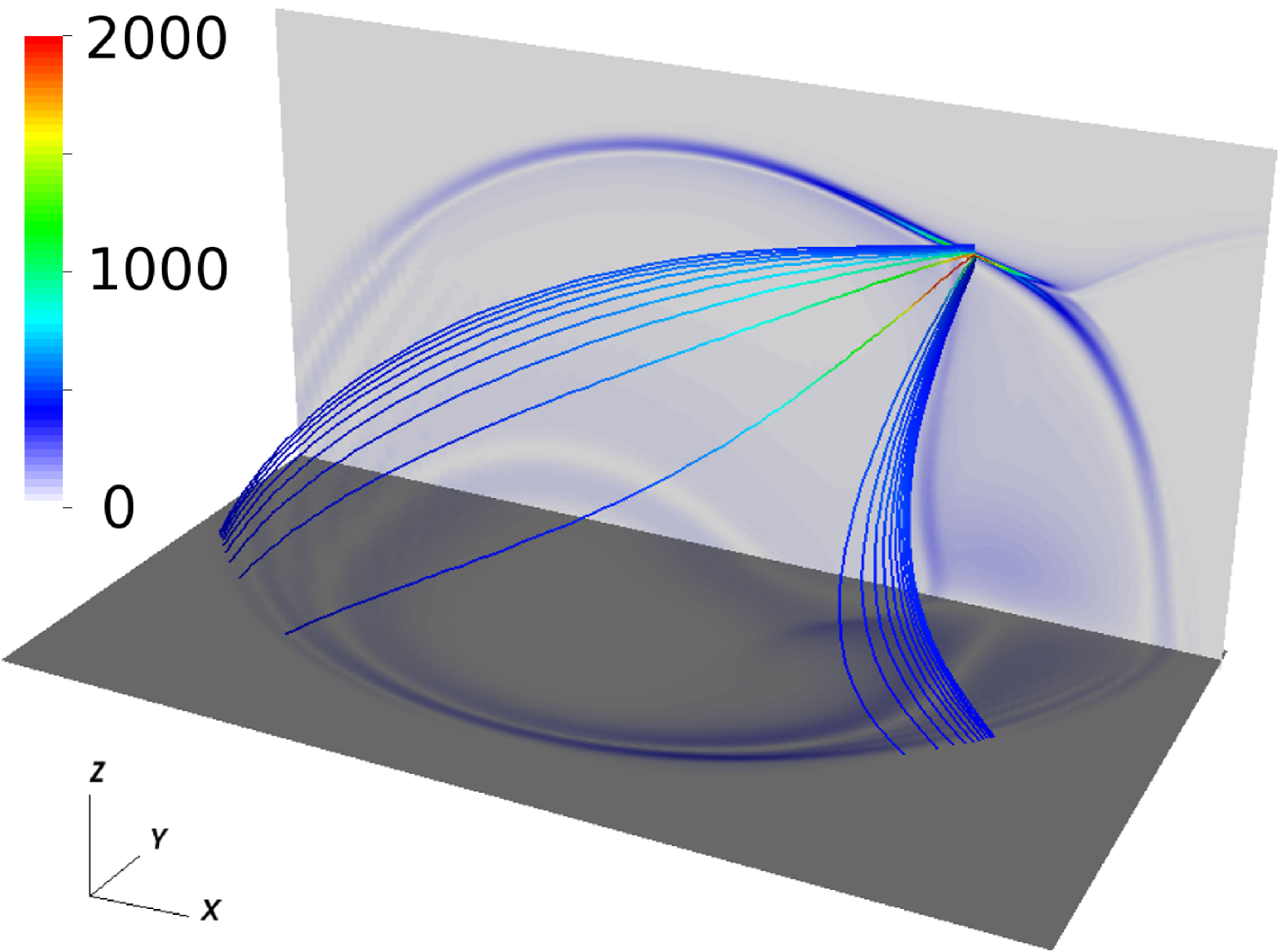
Finally, we remark that the assumption of a quasi-stationary evolution loses its validity in the late stage of the sheet evolution: Obviously, the collapse becomes a localized, dynamic process associated with significant magnetic forces. This can be seen from the field line plot shown in Fig. 6, where magnetic field lines connecting the thin current sheet with the photosphere have been colored with the quantity . For a force-free field, , the value of is constant along magnetic field lines. This condition is obviously not met in the QSL, which means that the currents close locally across field lines.
IV Conclusions
We carried out numerical simulations of current sheet formation in a quasi-separatrix layer using a simplified MHD model appropriate for the quasi-static evolution of a low- plasma. The setting under consideration has been investigated before Aulanier et al. (2005) and our results agree well with that work as long as the current sheet structure is well resolved in both studies. With the use of local adaptive mesh refinement (AMR), we were able to follow the thinning of the current sheet further down to a scale which is about one order of magnitude smaller than previously investigated. In particular, our simulations reached a stage in which the maxima of in the upper part of the QSL grow significantly beyond the values close to the photospheric boundaries, which gives clear evidence that the most intense current densities actually can be expected in the upper part of the QSL. This late stage is characterized by a relatively fast collapse of the locally almost one-dimensional sheet with an approximately exponential increase of in time, and the evolution is no more quasi-static at this point.
When magnetic forces become significant in this late stage of the current sheet formation, full nonlinear MHD dynamics will take place. Previous studies have addressed details of the local dynamics of such current sheets using appropriate initial conditions and periodic systems (e.g. Grauer and Marliani (2000) and references therein). There, one particular question has been whether the current density might form a singularity in finite time, or whether its growth is limited to merely e.g. exponential behavior. On theoretical grounds, it could be shown that a dynamical alignment between the velocity and the magnetic field would bound to exponential growth. Analyzing our data further, we actually found indications of such an alignment (not shown here), so that we expect to see a collapse of the sheet with exponential growth, i.e. a continuation of the phase observed between and in Fig. 3, given that it could be resolved numerically. At present however, even our AMR simulations are limited by the lack of further resolution and by numerical side-effects like artificial stabilizing diffusion.
The plasma flow pattern has been analyzed in a cut plane that is approximately perpendicular to the local direction of the current density in the sheet: If transformed into a frame that moves with the expanding structure, it exhibits a shear pattern which arises from a vortex below and a large-scale flow above. The vortex maps to the vortical boundary driver, while the large-scale flow is related to the slow overall expansion of the magnetic structure.
In this paper, we have only addressed the case of one specific boundary perturbation, namely a twisting motion at the footpoints. We have also conducted a number of simulations with a translational motion analogous to that used in Aulanier et al. (2005), and observed comparable behavior in these cases as well. In particular, the achieved current densities continued to rise at similar rates until they were restricted by finite grid resolution.
Acknowledgements.
The authors would like to thank G. Aulanier for helpful discussions during the preparation of the manuscript, and an anonymous referee for comments that helped to improve it. This work was supported by Deutsche Forschungsgemeinschaft through Forschergruppe FOR 1048 and by the European Commission through the Solaire network (MTRN-CT-2006-035484).References
- Démoulin et al. (1996a) P. Démoulin, J. C. Henoux, E. R. Priest, and C. H. Mandrini, Astronomy and Astrophysics 308, 643 (1996a).
- Démoulin et al. (1996b) P. Démoulin, E. R. Priest, and D. P. Lonie, J. Geophs. Res. 101, 7631 (1996b).
- Milano et al. (1999) L. Milano, P. Dmitruk, C. Mandrini, and D. Gómez, Astrophys. J. 521, 889 (1999).
- Titov and Hornig (2002) V. S. Titov and G. Hornig, Adv. Sp. Res. 29, 1087 (2002).
- Titov (2007) V. S. Titov, Astrophys. J. 660, 863 (2007), eprint arXiv:astro-ph/0703671.
- Titov et al. (2003) V. S. Titov, K. Galsgaard, and T. Neukirch, Astrophys. J. 582, 1172 (2003).
- Galsgaard et al. (2003) K. Galsgaard, V. S. Titov, and T. Neukirch, Astrophys. J. 595, 506 (2003).
- Aulanier et al. (2005) G. Aulanier, E. Pariat, and P. Démoulin, Astronomy and Astrophysics 444, 961 (2005).
- Aulanier et al. (2006) G. Aulanier, E. Pariat, P. Démoulin, and C. R. Devore, Sol. Phys 238, 347 (2006).
- Dreher and Grauer (2005) J. Dreher and R. Grauer, Parallel Computing 31, 913 (2005).
- Arnold et al. (2008) L. Arnold, J. Dreher, R. Grauer, H. Soltwisch, and H. Stein, Phys. Plasmas 15, 042106 (2008).
- Dedner et al. (2002) A. Dedner, F. Kemm, D. Kröner, C. Munz, T. Schnitzer, and M. Wesenberg, Journal of Computational Physics 175, 645 (2002).
- Shu and Osher (1988) C. Shu and S. Osher, J. Comp. Phys. 77, 439 (1988).
- Grauer and Marliani (2000) R. Grauer and C. Marliani, Phys. Rev. Lett. 84, 4850 (2000).