Numerical simulation of organic semiconductor devices with high carrier densities
Abstract
We give a full description of the numerical solution of a general charge transport model for doped disordered semiconductors with arbitrary field- and density-dependent mobilities. We propose a suitable scaling scheme and generalize the Gummel iterative procedure, giving both the discretization and linearization of the van Roosbroeck equations for the case when the generalized Einstein relation holds. We show that conventional iterations are unstable for problems with high doping, whereas the generalized scheme converges. The method also offers a significant increase in efficiency when the injection is large and reproduces known results where conventional methods converge.
pacs:
02.60.Cb,61.72.uf,81.05.Fb,02.60.LjI Introduction
Organic semiconducting materials have been the subject of much attention in recent years due to the prospect of tailoring their photoelectric properties to specific applications.1; 2; 3 Doping organic semiconductors, by embedding electron- or hole-donor species in the material, provides a particularly effective way of tuning device properties.4 Dopant concentrations can be easily and precisely controlled, although the effect on device performance is not always known a priori.
Simulation is a powerful tool for understanding and optimizing device performance, allowing systematic studies of device design that are experimentally infeasible. Computational approaches taken by other authors include Monte Carlo simulation,5 master equation approaches,6 and solution of the one-dimensional drift-diffusion-Poisson system of equations,7 which is the approach we follow here. This last approach is highly suited to the extraction of model parameters from experimental data and device optimization, since it is less computationally-expensive than methods dealing with more dimensions. One-dimensional drift-diffusion models originate from the theory of conventional crystalline semiconductors. However, when combining models for disordered materials with high doping intensities, numerical approaches originally developed for inorganic crystalline materials may fail. We derive a generalization of existing methods, namely the Scharfetter-Gummel discretization8 and the Gummel-iteration map9, to overcome these problems and then compare our results with a state-of-the-art simulation approach presented in Ref. 10. The numerical scheme that we develop here improves the numerical stability and computational efficiency of the approach.
The rest of this paper is structured as follows: In Sec. II, we introduce a model for steady-state charge transport in disorded semiconductors. In Sec. III, we describe a scaling scheme to improve numerical behavior. We present in Sec. IV the proper Scharfetter-Gummel discretization of the model, accounting for the generalized Einstein relation. In Sec. V, we derive the appropriately generalized Gummel iteration for the model. Numerical data for three example calculations are given in Sec. VI, comparing the proposed method with that of Ref. 10. Finally, we draw our conclusions in Sec. VII. The procedure is written for hole-transporting and bipolar devices in Appendix A, and the scaling factors we use are tabulated in Appendix B. Throughout this article, we use the symbol for the elementary charge.
II Mathematical model
The starting point for the derivations of most macroscopic charge transport models in semiconductors is the drift-diffusion-Poisson system introduced for inorganic crystalline semiconductors by van Roosbroeck,11
| (1) | ||||
| (2) | ||||
| (3) | ||||
| (4) |
Here, is the particle current, is the density, is the electrostatic potential, is the dopant density (assumed to be positive in case of -type doping), is the electron mobility, and is the diffusion constant. The subscripts and refer to electrons and holes, respectively, and the total charge current is given by . To simplify the notation, we write the equations henceforth only for electrons using the electron density . The following derivation is equally applicable for holes, since the equations in this case only differ by the sign of the drift term in the continuity equation and the carrier density in the Poisson equation. Appendix A gives the extension of our results to bipolar and hole-transport devices.
The model of Eqs. 1–4 was derived for crystalline silicon-based semiconductors12 and has been applied in that area for many years with great success. Although there is no ab initio derivation, application of Eqs. 1–4 to organic semiconductors seems promising since the charge continuity and Poisson equations intuitively apply in some form. Similar models are used for organic electronics in, e.g., Refs. 10; 13.
In fact, Eqs. 1–4 must be extended in order to accurately describe disorded organic semiconductors.14 Available models include the extended Gaussian disorder model (EGDM) and the extended correlated disorder model (ECDM).15; 16 Both models assume a hopping mechanism for charge transport with a Gaussian density of states. The EGDM and ECDM introduce density- and field-dependence into the mobility and diffusion coefficients and , respectively. The methods that we present in Secs. III, IV and V are applicable to arbitrary and ; here we discuss the EGDM and ECDM since they are recent and popular models.
It should be noted that in the context of so-called deep traps, introduced e.g. in Refs. 10; 17, the trapped carriers act as a stationary background charge and their treatment is completely analogous to the doping. Our method should therefore also lead to better performance in situations where deep traps are considered.
We restrict the discussion to one-dimensional steady-state current simulations. It is useful to introduce the functions and , writing the steady-state system as
| (5) | ||||
| (6) |
where is the temperature. When the system is accurately described by Maxwell-Boltzmann statistics, the classical Einstein relation holds,
| (7) |
with the thermal voltage . Note that in this equation the Boltzmann constant is taken to have units . In order to align notation with other authors in the field, we will frequently use in units of . To still be able distinguish these two conventions we will use in this case.
When facing high charge-carrier densities, the effects of the Pauli exclusion principle become important and one is forced to resort to Fermi-Dirac statistics. In the context of organic semiconductors, it was first pointed out by Roichmann and Tessler18 that one should then use a generalized version of Eq. 7,
| (8) |
where is the electron quasi-Fermi level (sometimes referred to as the chemical potential; we use the term quasi-Fermi level to avoid confusion and to stress that it is a non-equilibrium quantity). Within the EGDM/ECDM framework, Eq. 8 is usually written as
| (9) |
and is termed the diffusion enhancement. We adopt this convention for clarity and compatibility with other authors.
For a given density, the quasi-Fermi level is defined implicitly by the identity
| (10) |
where DOS() represents the density of states.
Equation 8 is called the generalized Einstein relation19 and accounts for the fact that charge carriers near the quasi-Fermi level are more likely to contribute to diffusion. The derivative occurring in Eq. 8 can be computed analytically by differentiating Eq. 10. The differentiated expression can be found in e.g., the Appendix of Ref. 20.
III Scaling
In SI units, the absolute values of the carrier density and electrostatic potential can differ by over orders of magnitude. To avoid numerical problems we thus rescale the equations. Several scaling schemes have been proposed by other authors for both inorganic crystalline and organic devices.21; 22 We find that the scaling leading to the most stable behavior is state-dependent.
We suggest scaling the density by its maximum value (taking doping into account). We refer to the density scaling factor as . Since we use a thermionic injection model 23, which can be coupled with barrier lowering 24, the boundary values and therefore maxima of the density are not known a priori. The scaling is therefore applied at every iteration. The potential is scaled by , the maximum value of (the absolute value of) the applied voltage and the thermal voltage. This ensures that the scaled potential is reasonably small even for high applied voltages. On the other hand, we force the scaling parameter to be at least the thermal voltage to avoid scaling by zero. Since the mobility may differ strongly between materials, we scale all mobilities by their zero-field, zero-density limit . Finally, space is scaled by , the total thickness of the device. The full list of the scaling parameters including the resulting scaling of the current density is given in Table 2.
The scaled system of equations reads (using the same symbols for the scaled quantities)
| (11) | ||||
| (12) |
where we have used the constants
| (13) |
Here, is the scaled Debye length.
This scaling ensures that the potential and density vary between and for most physical situations. Failing to implement a suitable scaling scheme can result in numerical instability and loss of accuracy. Furthermore, it reduces the number of constants used in the actual computations. Except where explicitly stated, we henceforth use the scaled quantities.
IV Discretization
To solve Eqs. 5 and 6 (note that these are the unscaled equations), Scharfetter and Gummel8 proposed a scheme for the case of constant mobility and diffusion. Instead of using central or upwind differences to approximate the current, a weighted difference depending on the field is used. It can be derived as a solution of the boundary value problem (BVP)
| (14) |
which describes the physics on a sub-interval for given carrier densities at the boundaries. The BVP of Eq. 14 is first order, but we can prescribe two boundary values because is a free parameter of the system, and there is only one value of that admits a solution. This value can be used as an approximation of the current, assuming that the mobility, diffusion coefficient and electric field are locally constant. Expressed in terms of and , it reads
| (15) |
The scheme can be viewed as an upwind scheme, where the amount of upwind difference depends on the local strength of the field. This is easily seen by considering the asymptotic behavior of when the field is large or small,
| (16) |
so that for small fields we use a classic central difference approximation for the gradient of the density, i.e., the diffusive part of the current. When the magnitude of the field is large, we obtain
| (17) |
and
| (18) |
which are exactly upwind approximations for the density.
Upwind schemes introduce artificial diffusion into the solution,25 which is a source of error. In the case of constant mobility and the simple Einstein relation of Eq. 7, it can be proven that the discretization introduced in Eq. 15 yields the optimal artificial diffusion (i.e., the minimum required for numerical stability). 26
Within high-density capable models such as EGDM/ECDM, the generalized Einstein relation of Eq. 8 increases physical diffusion. Use of Eq. 15 to approximate the current is then suboptimal in terms of the accuracy of the solution because more artificial diffusion is added than is required for stability. Using the generalized Einstein relation Eq. 8 and applying the scaling introduced in Sec. III, we obtain the following generalization of the BVP of Eq. 14,
| (19) |
This corresponds to the current in Eq. 11.
Assuming , and to be constant on each interval, or put equivalently, approximating them by their value at , we solve Eq. 19 as before to get a properly-adjusted discretization scheme,
| (20) |
This scheme accounts for the additional physical diffusion in our system by decreasing the artificial diffusion, improving the accuracy of the current.
In the EGDM/ECDM, . In this case and at half-integer gridpoints can be obtained by various averaging methods. Throughout this work we use the geometric average
| (21) |
which is an exact interpolant for exponentially varying functions. Note that since depends on the gradient of the potential, it is already known on half-integer gridpoints only.
V Iterative solution of the discretized system
To solve the system of discretized equations, Eqs. 5 and 6, using the discretization of Sec. IV, one can either use the Newton algorithm or the so-called Gummel iteration, a physically-motivated variant of the Gauss-Seidel relaxation scheme.9
Numerical comparisons as in the work of Knapp et al.27 and additional theoretical considerations show that Newton’s method converges in fewer iterations than the Gummel method. However, Newton iterations are generally more expensive to compute. Furthermore, Newton’s method often requires initial values in the vicinity of the solution in order to obtain convergence.
This is a severe problem for optimization and parameter extraction, where the solver is routinely called several hundred times. In these cases a single failure to converge can be catastrophic for the optimizer. We therefore derive an iterative solution scheme in the spirit of Gummel.9 As a starting point we will use the continuous (non-discretized) problem to avoid working in spaces of grid functions.
The idea is to alternately solve for at a given and for and given until self-consistency is achieved.
Since the drift-diffusion-Poisson system of equations can be nonlinear (even when and are constant; there is implicit dependency of e.g., on ), we must linearize first. Our iteration starts with the Poisson equation.
V.1 Linearization of the Poisson equation
The essence of the Gummel iteration is to consider the implicit nonlinearity of the Poisson equation explicitly, i.e.,
| (22) |
In the original derivation, the nonlinearity of in is revealed by the explicit use of Maxwell-Boltzmann statistics. This does not apply in our case, and we must use Eq. 10 instead. However, since even in Eq. 10 the dependence on is not explicit, we must first introduce another quantity, the quasielectrochemical potential , as defined in e.g., Ref. 28,
| (23) |
The quantity can be interpreted as the single driving potential for the charge carrier transport. One must be aware that there are several conventions in defining these levels, which are not consistent with each other. We use the distinction between the different levels as introduced in Ref. 28. However, we use a definition of the quasi-Fermi level consistent with Ref. 20, since the -prefactor that we use in our computations is introduced there. Therefore, the quasi-Fermi level and quasielectrochemical potential are switched with respect to those of Ref. 28. The difference stems from the choice of reference point with respect to which we define the DOS. We need here to reformulate the Gauss-Fermi integral of Eq. 10. Since this equation uses an unscaled we need to unscale our variable when we put it in
| (24) |
where is the site density. We deliberately use here instead of because its numerical value is . This can be understood from the consideration that all energies in the numerator of the exponential in Eq. 24 are in units of , whereas the product has unit . These units differ by the numerical value of the elementary charge , hence in Eq. 23 is and can be omitted in numerical calculations.
We find it useful to define the ’Poisson equation operator’
| (25) |
which we wish to linearize at the current iterate , where denotes iteration number. To avoid unnecessarily lengthy formulas, we introduce the notation
| (26) |
The linearization is performed using functional derivatives,29
| (27) |
The term is understood as a (pointwise) multiplication operator. Since the central difference approximation of the Laplacian and the pointwise approximation of are linear and continuous as projections onto finite dimensional spaces, the discretization commutes with the linearization.
The derivative is straightforwardly related to the factor. Comparing Eqs. 10 and 24, we get
| (28) |
We can rewrite the derivative with respect to ,
| (29) |
which leads to
| (30) |
Equation 30 is highly convenient, since and are computed elsewhere and can be reused here at virtually no cost. The linearization process thus doesn’t require computation of any additional quantities.
Using Eq. 30, we get for the derivative of the Poisson-operator
| (31) |
To complete the linearization, we insert this result into Eq. 27, set Poiss and , and solve for . This yields
| (32) |
We now switch back to the discretized system. As mentioned before, the order in which we linearize and discretize does not matter. We discretize using the following expressions,
| (33) | ||||
| (41) |
and solve for , setting the first and the last (spatial grid) values of the quantity in the square brackets of Eq. 32 to the boundary values. The boundary values of and are determined by the applied voltage and the charge injection, respectively. The matrix elements not shown in Eq. 41 are zero.
Equation 32, which we derived by linearizing the poisson operator, properly generalizes the Gummel iteration scheme to the case of a generalized Einstein relation.
V.2 Linearized Continuity equation
Since it is comparatively straightforward, we give the linearization for the continuity equation on the discretized level. We do not consider the implicit nonlinearity via here, and linearize the mobility by assuming that , the mobility at the -th iteration, depends on and not . Before giving the full expression for the linearized and discretized current, it is convenient to introduce the function
| (42) |
Substituting this definition into Eq. 20, the discretized and linearized current is given by
| (43) |
This expression is linear in . Therefore the central approximation of the continuity equation , which is what is solved in practice, is clearly also linear in . Equations 32–43 define the discretized and linearized system and are accessible to direct solution methods.
A diagram illustrating the iteration scheme resulting from the linearizations presented in the preceding sections can be found in Fig. 1.
VI Simulation results
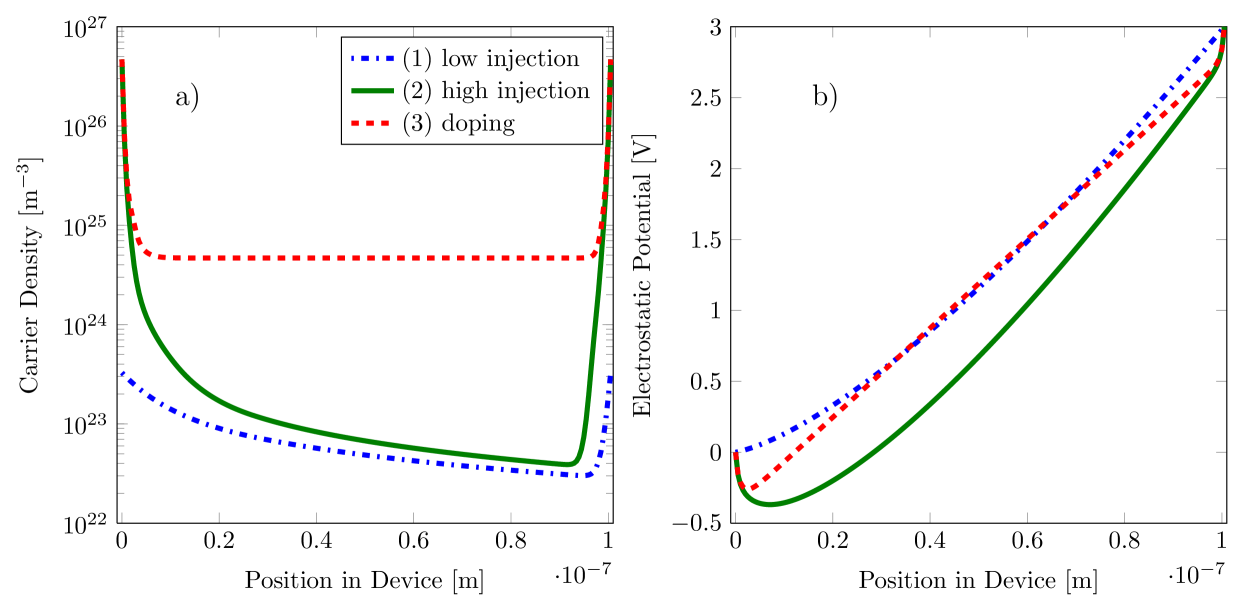
To highlight the advantages of the schemes described above, we have simulated a simple single-layer structure using the ECDM model. We consider three different situations: First, we simulate a low density situation without doping — here we show that our approach reproduces known results with a small gain in computational efficiency. Second, we simulate a device with high carrier densities due to a low injection barrier — here we observe a significant performance gain with the proposed method. Finally, we simulate a strongly-doped device, with approximately every th molecule replaced by a dopant. In this third case, conventional methods fail but our procedure converges. The parameters used for the simulations are collected in Table 1. The resulting charge carrier densities and potentials at are shown in Fig. 2. All of the device simulations, including those using the conventional iteration, used the discretization described in Sec. IV and had identical initial values. Our calculations did not include the barrier-lowering effect of image-charges in the metal contacts. Its inclusion would have the effect of increasing the carrier injection, further enhancing the computational advantage of our method.
| Parameter | (1) | (2) | (3) |
|---|---|---|---|
| Electrode WF [eV] | -5 | -4.6 | -4.6 |
| Doping intensity | |||
| Mobility model | ECDM | ||
| Injection model | Thermionic | ||
| LUMO [eV] | -4.5 | ||
| Site density [m-3] | |||
| DOS width [eV] | 0.13 | ||
| Temperature [K] | 300 | ||
| Device Length [nm] | 100 | ||
| ECDM-C parameter | 0.29 | ||
| [m2(Vs)-1] | |||
VI.1 Convergence
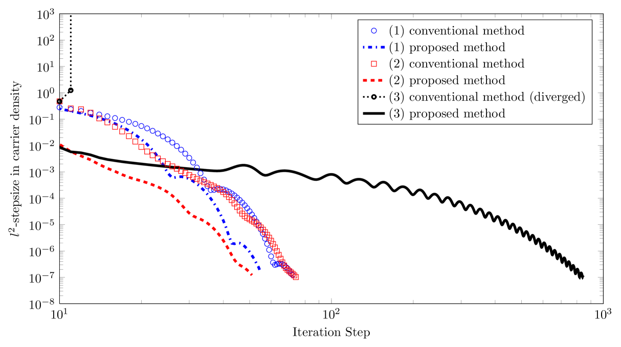
In Fig. 3, we compare the behavior of the method proposed in this paper, with the method presented by Knapp et al.,10 which we call the ’conventional method’.
The main difference between the approaches lies in the linearization of the Poisson equation. Knapp et al. use the expression (written in the framework of our scaling for the reader’s convenience)
| (44) |
instead of Eq. 32. This differs from Eq. 32 by the absence of in the denominators and the doping profile, which wasn’t considered in Ref. 10. The effect can be viewed as a different damping. However, one should keep in mind that our scheme is not derived from a perspective of damping but from the use of functional derivatives for the Poisson operator introduced in Eq. 25.
A similar difference can be seen in the discretization of the continuity equation, where an additional turns up in the denominator of the argument of the exponential function. As mentioned above, this prevents the introduction of unnecessary artificial diffusion.
In all three device simulations, the proposed method is superior to the conventional method in terms of convergence speed, with the difference being greater when the carrier densities are high. Our convergence criterion was that the -stepsize in the scaled charge density fall below .
We find that the stability of the generalized iteration in high-concentration regimes is greatly enhanced in comparison with the conventional iteration. For example, the conventional approach fails to converge for doping intensities , whereas our method converges for arbitrary doping intensities. The benefits of properly incorporating diffusion into the numerical scheme could also be important for the simulation of multilayer devices, and in particular those with doped layers.
Even in the absence of doping, for large values of charge carrier injection a speed-up of convergence is observed. In the low density limit, the method blends into the one presented in Ref. 10 because , as .
VI.2 Grid convergence
Since we introduced a scheme using upwind stabilization, it is interesting to study the effect of varying gridpoint density on the behavior of the solution. We have studied the effect of the number of gridpoints on the current density for the three cases shown in Table 1. We investigate uniform grids with up to gridpoints.
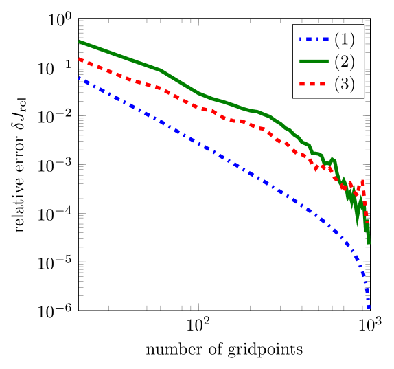
As shown in Fig. 4, we observe convergence using the proposed method in all three cases. However, for high carrier densities the relative error in the current oscillates slightly with varying grid resolution. This is likely to be a result of the averaging procedure used on the mobility prefactors , and is a topic for further investigation. The oscillations are, however, smaller than the general trend of convergence.
VII Summary and Conclusions
We have introduced a numerical method consisting of a scaling scheme, a discretization scheme, and a fixed point iteration for the van Roosbroeck drift-diffusion-Poisson system with arbitrary density- and field-dependent mobility functions. The method properly accounts for the implications of Fermi-Dirac statistics by incorporating the generalized Einstein relation. The iteration is derived by linearizing the Poisson equation with explicit treatment of the nonlinear dependence of the density on the potential.
Failure to take consequences of the generalized Einstein relation into account in the iteration results in numerical instability when the density is large, e.g., in the case of strong doping or large trap density, whereas the generalized method converges for arbitrary doping. In other cases, we find that the generalized method is significantly more efficient than the conventional method while reproducing converged current values.
Acknowledgements.
We thank René Pinnau from TU Kaiserslautern for fruitful discussions. C.K.F. Weiler acknowledges funding from the BMBF project PARAPLUE, project number 03MS649A.Appendix A Numerical Scheme for positive carriers
While the modelling details of bipolar devices (charge generation/recombination) are outside the scope of this paper, we show how to extend the method presented above to hole-transporting or bipolar devices. For the iterative procedure, we include a hole continuity equation, which has the same mathematical form as the electron continuity equation, except the sign of the drift term is changed. As for electrons, we use Scharfetter-Gummel for the discretization and linearize the mobility by using the values of the last iteration. The analogue of Eq. 43 for holes is
| (45) |
This allows us to solve the for the new iterate in the same way as we did for the electron density in Sec. V. In the linearization of the Poisson equation, we do not only need to linearize but in an analogous manner also . The effect of the potential on the two carrier densities is the same except for a reversed sign, i.e., the hole analogue of Eq. 28 has a minus sign. However, since and appear in the poisson equation with different signs, they appear in the linearized iteration in the prefactor multiplying on the same footing (i.e., or ). We obtain
| (46) |
Here, the linearized Poisson operator reads
| (47) |
The discretization and solution of the Poisson equation then works exactly as described in Sec V.
Appendix B Scaling factors
Here we list the model scaling factors, which we use to force densities and potential to vary between zero and one. Note that the density and current scaling factors have the potential to change during the calculation, so should be updated after every iteration.
| Variable | Symbol | Scaling factor |
|---|---|---|
| Potential | ||
| Density | ||
| Length | ||
| Mobility | ||
| Current |
References
- Pron et al. (2010) A. Pron, P. Gawrys, M. Zagorska, D. Djurado, and R. Demadrille, Chem. Soc. Rev. 39, 2577 (2010).
- van Mensfoort et al. (2011) S. van Mensfoort, J. Billen, M. Carvelli, S. Vulto, R. Janssen, and R. Coehoorn, J. Appl. Phys. 109, 064502 (2011).
- Anthony et al. (2010) J. E. Anthony, A. Facchetti, M. Heeney, S. R. Marder, and X. Zhan, Adv. Mater. 22, 3876 (2010).
- Chan et al. (2009) C. Chan, W. Zhao, A. Kahn, and I. Hill, Appl. Phys. Lett. 94, 203306 (2009).
- van der Holst et al. (2011) J. van der Holst, F. van Oost, R. Coehoorn, and P. Bobbert, Phys. Rev. B 83, 085206 (2011).
- van Mensfoort et al. (2010) S. van Mensfoort, V. Shabro, R. de Vries, R. Janssen, and R. Coehoorn, J. Appl. Phys. 107, 113710 (2010).
- Cottaar, Coehoorn, and Bobbert (2012) J. Cottaar, R. Coehoorn, and P. Bobbert, Org. Elec. 13, 667 (2012).
- Scharfetter and Gummel (1969) D. Scharfetter and H. Gummel, IEEE T. Electron. Dev. 16, 64 (1969).
- Gummel (1964) H. Gummel, IEEE T. Electron. Dev. 1, 455 (1964).
- Knapp et al. (2010) E. Knapp, R. Häusermann, H. Schwarzenbach, and B. Ruhstaller, J. Appl. Phys. 108, 054504 (2010).
- van Roosbroeck (1950) W. van Roosbroeck, Bell System Tech.J, 29, 560 (1950).
- Juengel (2009) A. Juengel, “Drift-diffusion equations,” (Springer, 2009) Chap. 5, pp. 99–127.
- Xu et al. (2011) Y. Xu, T. Minari, K. Tsukagoshi, R. Gwoziecki, R. Coppard, M. Benwadih, J. Chroboczek, F. Balestra, and G. Ghibaudo, Journal of Applied Physics 110, 014510 (2011).
- Scher, Shlesinger, and Bendler (1991) H. Scher, M. F. Shlesinger, and J. T. Bendler, Phys. Today 44, 26 (1991).
- Coehoorn et al. (2005) R. Coehoorn, W. F. Pasveer, P. A. Bobbert, and M. A. J. Michels, Phys. Rev. B 72, 115206 (2005).
- Bouhassoune et al. (2009) M. Bouhassoune, S. van Mensfoort, P. Bobbert, and R. Coehoorn, Org. Elec. 10, 437 (2009).
- Schober et al. (2011) M. Schober, M. Anderson, M. Thomschke, J. Widmer, M. Furno, R. Scholz, B. Lüssem, and K. Leo, Phys. Rev. B 84, 165326 (2011).
- Roichman and Tessler (2002) Y. Roichman and N. Tessler, Appl. Phys. Lett. 80, 1948 (2002).
- Ashcroft and Mermin (1976) N. W. Ashcroft and D. N. Mermin, Solid State Physics (Saunders College Publishing, 1976).
- van Mensfoort and Coehoorn (2008) S. L. M. van Mensfoort and R. Coehoorn, Phys. Rev. B 78, 085207 (2008).
- Brezzi et al. (2005) F. Brezzi, L. Marini, S. Michelettio, P. Pietra, R. Sacco, and S. Wang, “Handbook of numerical analysis, vol. xiii (numerical methods for electrodynamic problems),” (Elsevier Science, 2005) Chap. Finite element and finite volume discretizations of Drift-Diffusion type fluid models for semiconductors.
- Bonham and Jarvis (1977) J. Bonham and D. Jarvis, Aust. J. Chem. 30, 705 (1977).
- Scott and Malliaras (1999) J. Scott and G. G. Malliaras, Chemical Physics Letters 299, 115 (1999).
- Emtage and O’Dwyer (1966) P. R. Emtage and J. J. O’Dwyer, Phys. Rev. Lett. 16, 356 (1966).
- Smith (1985) G. Smith, Numerical Solution of Partial Differential Equations: Finite Difference Methods, Oxford Applied Mathematics And Computing Science Series (Clarendon Press, 1985).
- Doolan, Miller, and Schilders (1980) E. Doolan, J. Miller, and W. Schilders, Uniform numerical methods for problems with initial and boundary layers, Advances in numerical computation series (Boole Press, 1980).
- Knapp and Ruhstaller (2011) E. Knapp and B. Ruhstaller, Opt. Quant. Electron 42, 667 (2011).
- Woellner and Freire (2011) C. F. Woellner and J. A. Freire, J. Chem. Phys. 134, 084112 (2011).
- Courant and Hilbert (2007) R. Courant and D. Hilbert, “The calculus of variations,” in Methods of Mathematical Physics (Wiley-VCH Verlag GmbH, 2007) pp. 164–274.