Numerical solution of the relativistic single-site scattering problem for the Coulomb and the Mathieu potential

For a numerical treatment of equation (3) and (4) it is common to transform the large and the small component of the solution according to

By introducing the matrices $\underline{\underline{U}}^{+}(r)=\underline{\underline{V}}(r)-\varepsilon\,\underline{\underline{I}}_{4}$ and $\underline{\underline{U}}^{-}(r)=\left(\frac{\varepsilon}{c^{2}}+1\right)\,\underline{\underline{I}}_{4}-\frac{1}{c^{2}}\,\underline{\underline{V}}(r)$ as well as the spin-orbit coupling matrix $\underline{\underline{K}}=\left\{\kappa^{\prime}\delta_{\Lambda\Lambda^{\prime}}\right\}$, the following differential equations in matrix form are obtained,

Employing appropriate initial conditions the coupled equations (10) and (11) can be solved. After this step, the regular scattering solution has to be normalized at the boundary of the Wigner-Seitz cell according to equation (7). The normalized expansion coefficients of the regular single-site scattering solution inside the Wigner-Seitz cell $P^{\text{inside}}_{\Lambda^{\prime}\Lambda}(r)$ can be found as a linear combination of the numerically obtained solutions $P_{\Lambda^{\prime}\Lambda}(r)$,

By introducing the matrices $\underline{\underline{X}}(r_{\text{BS}})=\left\{r_{\text{BS}}x_{l}(kr_{\text{BS}})\delta_{\Lambda\Lambda^{\prime}}\right\}$ and $\underline{\underline{x}}(r_{\text{BS}})=\left\{r_{\text{BS}}ce_{\Lambda}x_{\overline{l}}(kr_{\text{BS}})\delta_{\Lambda\Lambda^{\prime}}\right\}$ ($x=j,h$) at the radius of the circumscribing sphere $r_{\text{BS}}$ of the Wigner-Seitz cell, the following algebraic system of linear equations can be formulated,

To discuss the numerical solution of the ordinary differential equations (10) and (11) we used Matlab [18] and compared the performance of seven different methods, which will be introduced briefly in the following. First of all, we used the standard solvers ode113 and ode15s, which are an Adams-Bashforth-Moulton predictor-corrector method of variable step size and variable order $1,\dots,13$ and an implicit method of variable step size and variable order $1,\dots,5$ based on the numerical differentiation formulas [19, 20]. Furthermore, the Dormand-Prince method [21] (ode45) and the Bogacki-Shampine method [22] (ode23) are used. Both solver are explicit methods of Runge-Kutta type with variable step size and orders 5 and 3, respectively. Since the Bulirsch-Stoer algorithm is used to solve the single-site scattering problem within some KKR codes, we included a Gragg-Bulirsch-Stoer algorithm (GBS) with both adaptive order and step size [23]. Last but not least, the fixed step size Runge-Kutta method of order 4 (RK4) and the fixed step size Adams-Bashforth-Moulton predictor corrector method of order 5 (AB5) are taken into account, since both are widely applied within the KKR community [24]. For the AB5 method, we use an explicit Adams-Bashforth method of order 5 as predictor which is corrected by an implicit Adams-Moulton method of order 5. The corrector step is repeated $n$ times, until the change of the solution due to the corrector step is smaller than a requested accuracy (PE(CE)ⁿ method). For RK4 and AB5 the ordinary differential equation was transformed analytically by assuming a logarithmic scale $x=\log(r)$.

Besides a direct solution of the differential equations (10) and (11) it is possible to solve the single-site scattering problem by means of integral equations. Suppose that the single-site scattering solution of the Dirac equation is known for an arbitrary reference system with the potential $\mathring{V}_{\text{eff}}(\vec{r})$. These solutions are denoted by $\mathring{\vec{\Psi}}_{\Lambda}(\vec{r})$, which could be either regular or irregular single-site scattering solutions. By using the Lippmann-Schwinger equation [25],

it is possible to calculate the solutions $\vec{\Phi}_{\Lambda}(\vec{r})$ corresponding to the potential $V_{\text{eff}}(\vec{r})=\Delta V(\vec{r})+\mathring{V}_{\text{eff}}(\vec{r})$. The quantity $\mathring{\underline{\underline{G}}}_{\text{S}}(E;\vec{r},\vec{r}^{\prime})$ in equation (14) denotes the single-site scattering Green function of the reference system and is constructed from the regular as well as the irregular single-site scattering wave functions $\mathring{\vec{R}}_{\Lambda}(E,\vec{r})$ and $\mathring{\vec{H}}_{\Lambda}(E,\vec{r}^{\prime})$ in the following way:

The quantities $\mathring{\vec{R}}_{\Lambda}^{n}(E,\vec{r_{n}})^{\times}$ and $\mathring{\vec{H}}^{n}_{\Lambda}(E,\vec{r}_{n})^{\times}$ denote the so-called left-hand side solutions, which were discussed in detail by Tamura [26]. By expanding the single-site scattering wave function in terms of the spin-angular functions (2) and by using equation (15), the Lippmann-Schwinger equation (14) for the regular and irregular single-site scattering wave functions can be reformulated in terms of the following matrix equations,

and

The matrices $\underline{\underline{A}}(z,r)$, $\underline{\underline{B}}(z,r)$, $\underline{\underline{C}}(z,r)$ and $\underline{\underline{D}}(z,r)$ contain the integrals over the radial amplitudes $g^{R,H}_{\Lambda^{\prime}\Lambda}(r)$ and $f^{R,H}_{\Lambda^{\prime}\Lambda}(r)$ as well as the functions $x^{R,H}_{\Lambda^{\prime}\Lambda}(r)$ and $y^{R,H}_{\Lambda^{\prime}\Lambda}(r)$, which include the solutions of the reference system and the change of the potential $\Delta V(\vec{r})$,

The explicit expressions of $x^{R,H}_{\Lambda^{\prime}\Lambda}(r)$ and $y^{R,H}_{\Lambda^{\prime}\Lambda}(r)$ are given by

In general, the Lippmann-Schwinger equation (14) is solved iteratively in terms of Born series by starting with the reference solution $\vec{\Phi}^{(0)}_{\Lambda}(\vec{r})=\mathring{\vec{\Psi}}_{\Lambda}(\vec{r})$ on the right hand side of equation (14) and by calculating a better approximation $\vec{\Phi}^{(1)}_{\Lambda}(\vec{r})$ by integration. This scheme is repeated, until the difference between two successive approximations, $\vec{\Phi}^{(n)}_{\Lambda}(\vec{r})$ and $\vec{\Phi}^{(n-1)}_{\Lambda}(\vec{r})$, is reasonably small.

The Coulomb potential is spherically symmetric and hence, the expansion into spherical harmonics only consists of one (spherically symmetric) component $V_{00}(r)$,

The associated ordinary differential equations are independent of the relativistic magnetic quantum number $\mu$ and diagonal in $\kappa$, but coupled with respect to $g_{\kappa}$ and $f_{\kappa}$,

It was pointed out by Swainson and Drake [27] that equations (28) and (29) can be decoupled by transforming the radial solutions according to

Here, the newly introduced quantities are given by $X=\frac{2(\gamma-\kappa)}{cZ}$ and $\gamma=\sqrt{\kappa^{2}-\frac{4Z^{2}}{c^{2}}}$. By using the abbreviations $\epsilon=\frac{W}{c}$, $\omega^{2}=(\frac{c}{2}-\frac{W}{c})^{2}$, and by combining equation (30) together with (28) and (29), two differential equations of second order can be obtained, which are similar to the form of the radial Schrödinger equation,

Close to the origin ($r\ll 1$), in the asymptotic limit, only the angular momentum terms ($\sim r^{-2}$) have to be taken into account, whereas the potential ($\sim r^{-1}$) and the constant factor $\omega^{2}$ can be neglected. The solution of the resulting differential equations are rational functions of the following form,

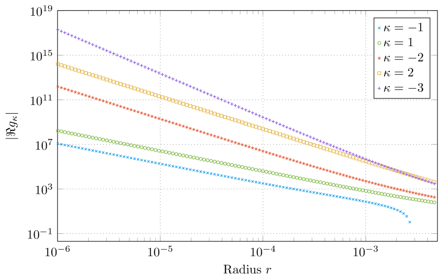
Since both solutions $g_{\kappa}$ and $f_{\kappa}$ are linear combinations of $\tilde{g}_{\kappa}$ and $\tilde{f}_{\kappa}$, it can be verified, that the leading term for the irregular solutions is given by $r^{-\gamma-1}$. In the non-relativistic limit ($\frac{4Z^{2}}{c^{2}}\approx 0$) the asymptotic behaviour of an irregular $s$-wave function ($\kappa=-1$, $l=0$) close to the origin is given by $r^{-\left|\kappa\right|-1}=r^{-2}$ which is in contradiction to the non-relativistic solution $r^{-l-1}=r^{-1}$. Since the relativistic quantum number $\kappa$ takes on values either $\kappa=l$ or $\kappa=-l-1$, this disagreement can be generalized for all irregular wave functions with $\kappa=-l-1$. To verify the solution behaviour for $r\ll 1$, a double logarithmic plot of the numerical solution for $Z=79$ and $c=\frac{2}{\alpha}$ and various values for $\kappa$ is illustrated in figure 1. The predicted asymptotic behaviour is clearly revealed.

For the discussion of the numerical accuracy for the solution of the differential equation (equations (31) and (32)), a Coulomb potential with an atomic number of $Z=79$ was used since it represents the element gold (Au). Due to the large atomic mass and non-negligible spin-orbit coupling, which causes the typical golden colour, it is a prominent example for relativistic effects. Solutions were obtained up to a maximal angular momentum quantum number of $l=5$. To obtain a scattering state, the energy of the scattering solution was chosen to be $\varepsilon=1$. In the following test, a spherical cell was constructed including a minimal radius of $r_{0}=10^{-4}$ and a maximal radius of $r_{\text{BS}}=3$.

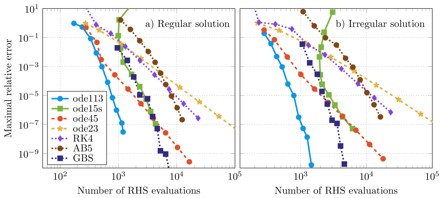
The numerical solutions obtained by using different solvers were compared with a reference solution, which was obtained by using ode113 and very high accuracy goals. For the solvers taken from the Matlab ode-suite absolute and relative tolerances were chosen to be equal and values between $10^{-1}$ and $10^{-10}$ were used. The maximal relative error of the numerically obtained solutions as a function of the number of right-hand side evaluations of the differential equation is shown in figure 2. First of all, it can be verified that the numerical accuracy of the solution of the regular single-site scattering solution (figure 3(a)) is similar to the results of the irregular single-site scattering solution (figure 3(b)). Hence, the following statements can be given for both types of solutions. As summarized by Söderlind et al. [28] an ordinary differential equation is called stiff, if the numerical solution via implicit methods performs much better than the solution via explicit methods. However, for the present example it can be verified that the method ode113, which is a method for non-stiff equations, performs better than the implicit method ode15s. Since we observed poor performance for other implicit methods, we conclude that the underlying differential equations for the Coulomb potential are non-stiff. The performance of the Dormand-Prince method (ode45) is very good for crude tolerances and becomes comparable to ode15s for fine tolerances. The Adams-Bashforth-Moulton predictor-corrector method of order 5 with fixed step size (AB5) is rather expensive for high tolerances. But, due to the higher order, the performance is better in comparison to the methods of the Runge-Kutta type ode23 and RK4, if high accuracy goals are demanded. Also in comparison to ode45, which has the same order, less evaluations of the right-hand side of the differential equation for high accuracy goals are necessary; it is therefore more efficient. The implemented Gragg-Bulirsch-Stoer method with both adaptive order and step-size (GBS) [23] is able to solve the differential equations with very high orders. But, for the accuracy goals in practice ($\approx 10^{-8}$) it needs about five times as many evaluations of the right hand side of the differential equation in comparison to ode113.

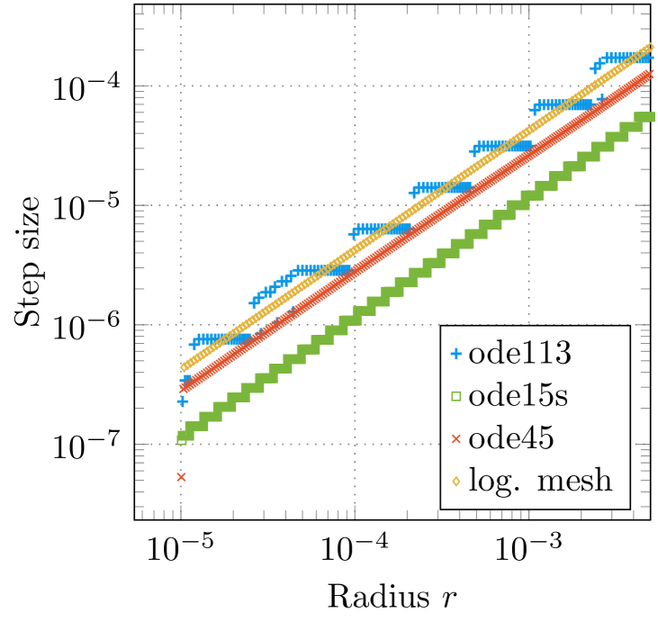
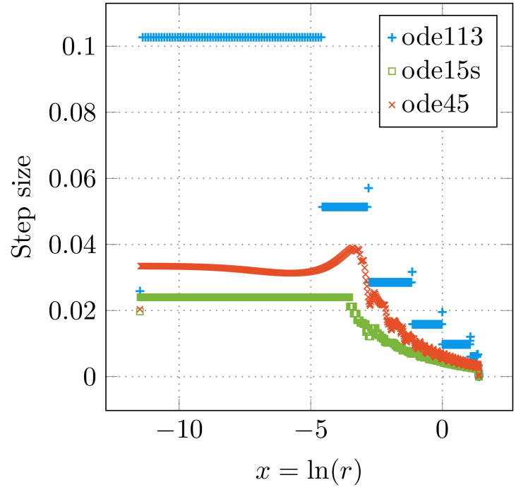
In many implementations of the KKR method, solvers with fixed step size are used for spherically symmetric atomic potentials, whereas a logarithmic mesh of type $x=\log(r)$ or similar is employed [24]. The reason for this is that the wave functions are highly oscillating close to the nucleus, and are smooth for larger values of $r$. To verify that a logarithmic mesh is a reasonable choice, the step size for adaptive methods close the origin was investigated (see figures 3(a) and 3(b)). The step size during the numerical solution of the Coulomb-Dirac problem using ode113, ode15s, and ode45 is illustrated in figure 3(a) and compared with the step size of a logarithmic mesh. It can be verified that the step size used by ode45 is similar to the characteristic of a logarithmic mesh. However, the stair-case-like behaviour of ode113 and ode15s occurs due to the step-size strategy of the method itself, i.e. the change of the step-size is avoided as much as possible [19]. Analogously, it is possible to transform the differential equations (31) and (32) to a logarithmic scale $x=\log(r)$ and to investigate the varying step size of the methods ode113, ode15s and ode45 for the numerical solution of the transformed equations (see figure 3(b)). It can be verified, that all three solvers adopt a constant step size close to the origin ($x<-5$), which again reassures the choice of a logarithmic scale for methods with fixed step size.

A suitable test system for our full-potential implementation is given by a Mathieu potential [29],

that is periodic and represents here a simple cubic crystal structure. Moreover, it is highly anisotropic with respect to different crystallographic directions and thus, it is ideal to serve as a test system. For our method it is necessary to express equations (35) in terms of complex spherical harmonics (see section 2). By using the exponential form of the cosine function and by applying Bauer’s theorem,

we end up with the following equation,

with coefficients $f_{lm}$ given by

Analogously to section 3.2, where the numerical accuracy was discussed for the Coulomb potential, our numerical test environment was used to solve the differential equations (10) and (11) for the Mathieu potential. According to Yeh et al. [29], the lattice constant was chosen to be $a=2\pi$ and the pre-factor $U_{0}$ was set to $U_{0}=-0.5$. The expansion of the solution in terms of spin-angular functions was evaluated up to a maximal angular momentum quantum number of $l_{\text{max}}=5$. Due to the high value of $l_{\text{max}}$ the matrices $\underline{\underline{P}}$ and $\underline{\underline{Q}}$ in (3) and (4) are of dimension $72\times 72$.

The maximal relative error between a very precise reference solution and the numerically obtained solution of different solvers versus the number of evaluations of the right-hand side of the differential equations are shown in figure 4. The general behaviour using different methods is similar for regular and irregular single-site scattering solutions. It can be verified that for a particular method and for the same number of evaluations of the right-hand side of the differential equation the maximal relative error for the regular solution is by approximately 2 orders of magnitude smaller compared to the irregular solution. This is due to very large absolute values of the irregular single-site scattering solutions close to the origin. As shown in the example for the Coulomb potential, we conclude that the underlying differential equations for the Mathieu potential can be regarded as non-stiff, since the performance of the method ode113 is much better than the performance of the method ode15s [28]. Again, the performance of the Adams-Bashforth-Moulton predictor-corrector method of order 5 (AB5) is worse than the explicit Runge-Kutta methods RK4 and ode45 for crude tolerances. However due to the higher order it is more efficient if high accuracy goals are required. Especially for the irregular solutions ode23 fails to give a reasonable solution for an appropriate amount of evaluations of the right-hand side of the differential equations.

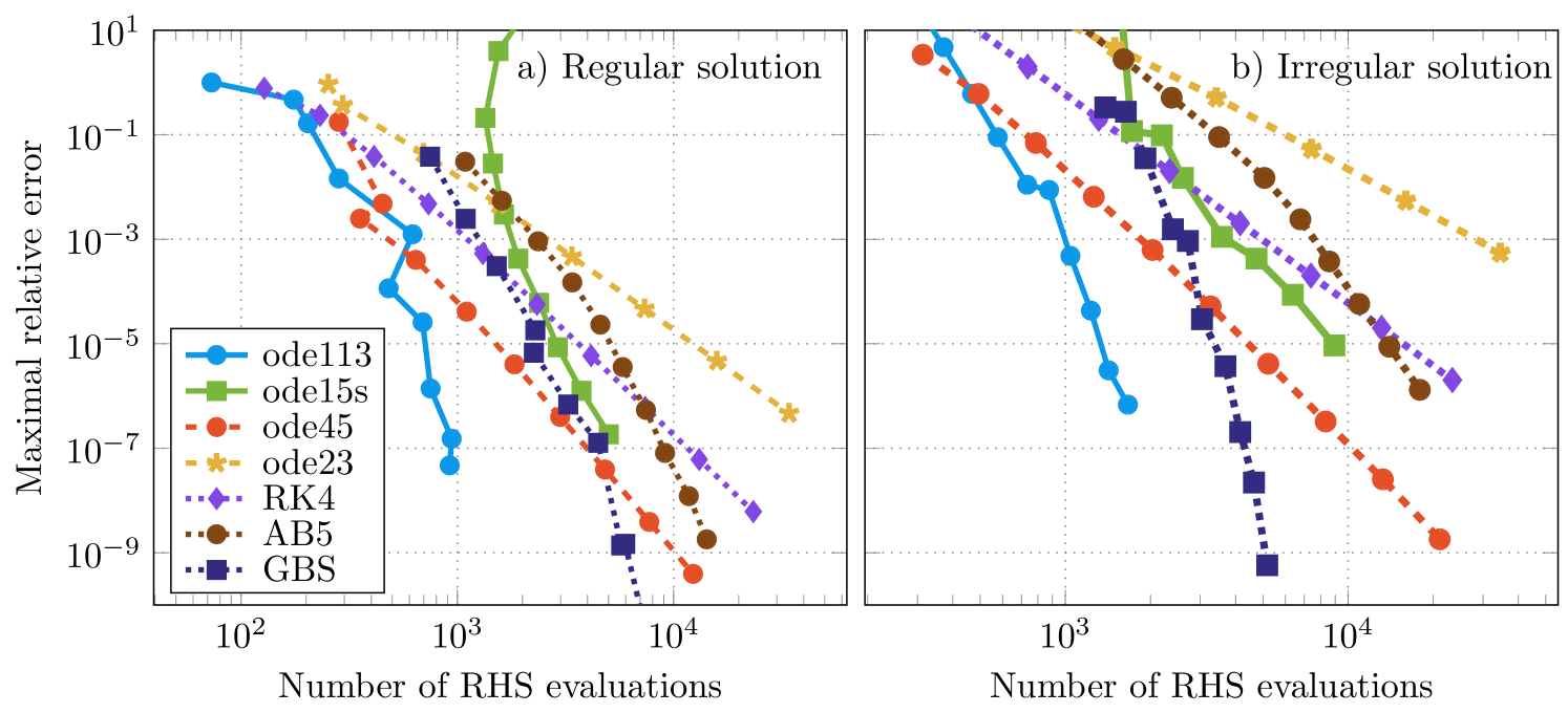
The differential equations (10) and (11) are characterized by the effective potential and since the Mathieu potential is analytically known, methods with adaptive step-size like ode113 are a reasonable choice. In general, the effective potential within each iteration of the KKR method is given on a discrete mesh and, hence, a method with fixed step size is appropriate, since interpolations of the potential between mesh points are avoided. For the Mathieu potential, it can be verified (see figure 4) that the numerical solution of the full-potential single-site scattering problem can be obtained by linear multi-step methods for non-stiff equations, e.g. by applying an Adams-Bashforth-Moulton predictor-corrector method. Therefore, the method AB5 was implemented within the computer code Hutsepot [30].

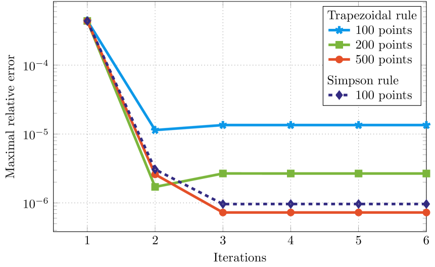
Besides the direct solution of the differential equation, the solution of the Dirac equation for a Mathieu potential was investigated by means of integral equations. For the integration, the trapezoidal rule as well as the Simpson rule was used. In figure 5 the maximal relative error of the solution is plotted versus the number of iterations within the Born series for the solution of the Lippmann-Schwinger equation for an irregular single-site scattering solution. It can be verified that the maximal relative error saturates quickly and the Born series converges after three iterations. This is in perfect agreement with the observation of Drittler [7] for the non-relativistic method. Since the deviation from the exact solution is dominated by the error of the numerical quadrature, the accuracy of the solution can be improved by either increasing the number of mesh points for the quadrature or by improving the integration scheme, e.g. using the Simpson rule instead of the trapezoidal rule. In this way the maximal relative error can be decreased by about one order of magnitude for the same number of points, where the integrand is evaluated.

After the solution of the Dirac equation at each atomic site $n$, the regular and the irregular single-site scattering solutions $\vec{R}^{n}_{\Lambda}(E,\vec{r}_{n})$ and $\vec{H}^{n}_{\Lambda}(E,\vec{r}_{n})$ can be used to construct the relativistic multiple-scattering Green function,

Analogously to the single-site scattering Green function (15), $\vec{R}_{\Lambda}^{n}(E,\vec{r}_{n})^{\times}$ and $\vec{H}^{n}_{\Lambda}(E,\vec{r}_{n})^{\times}$ denote the left-hand side solutions [26]. The matrix $\underline{\underline{g}}_{\Lambda\Lambda^{\prime}}^{nm}(E)$ is called structural Green function matrix and can be obtained from the structure constants $\underline{\underline{G^{0}}}(E)$ of the free space and the single-site scattering t-matrices $\underline{\underline{T}}(E)=\left\{\underline{\underline{t}}^{n}(E)\right\}$ at each site $n$,

Since the Green function has a singularity if the energy hits an eigenvalue of the Dirac Hamiltonian, the band structure of a system can be calculated by means of the Bloch spectral function, which is given by the imaginary part of the $\vec{k}$-resolved multiple-scattering Green function [31],

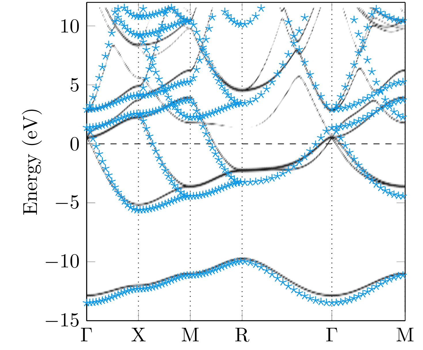
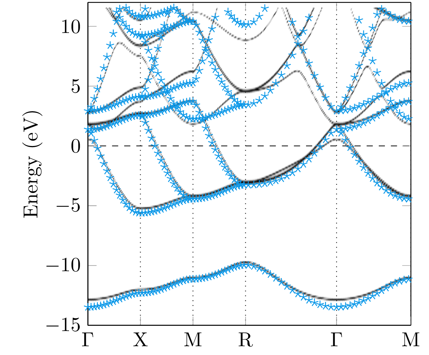
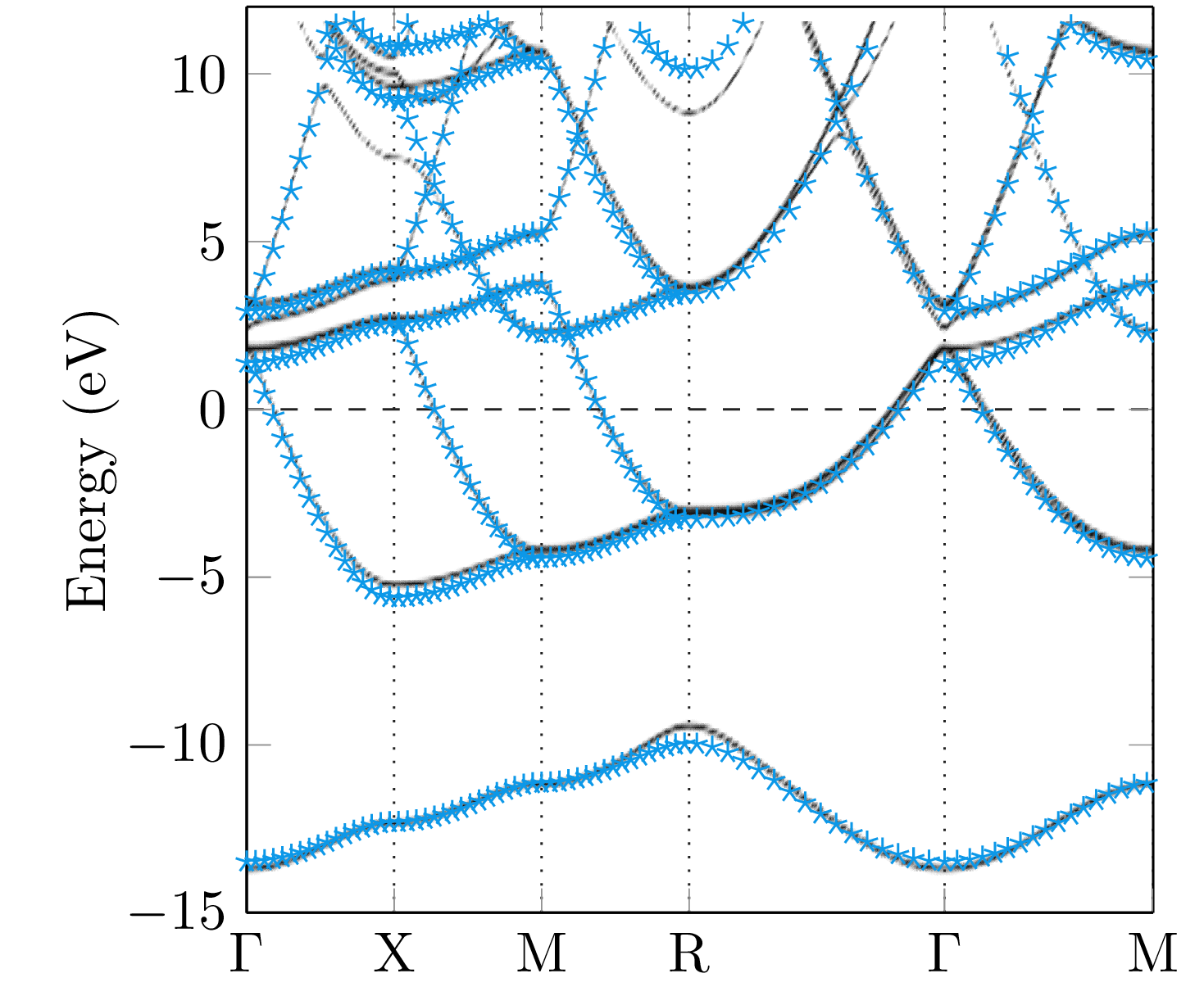
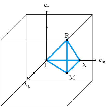
The summation in the last expression belongs to all lattice vectors $\vec{R}_{j}$ of the lattice denoted by $L$. The trace is a summation of the diagonal components of the $4\times 4$ dimensional Green function. The great advantage of the Mathieu potential is given by the fact, that the band structure can be calculated analytically and, therefore, it is a good test system for our numerical implementation. In general, a large number of terms are necessary within the angular momentum expansion of the Green function to obtain the correct energy bands. For illustrative purposes, the Bloch spectral functions obtained for different maximal angular momentum ($l_{\text{max}}=2,3,4$) within the expansion (39) together with the analytically obtained result are compared in Fig. 6. As can be seen, high values of $l_{\text{max}}$ are necessary to achieve a reasonable agreement between the band structures. However, the numerical result for $l_{\text{max}}=4$ reflects the general behaviour of the analytical band structure quite nicely.

References

- [1] P. Hohenberg and W. Kohn. Inhomogeneous Electron Gas. Phys. Rev., 136:B864–B871, Nov 1964.
- [2] J. Korringa. On the calculation of the energy of a Bloch wave in a metal. Physica, 13(6–7):392 – 400, 1947.
- [3] W. Kohn and N. Rostoker. Solution of the Schrödinger Equation in Periodic Lattices with an Application to Metallic Lithium. Phys. Rev., 94:1111–1120, Jun 1954.
- [4] H. Ebert, D. Ködderitzsch, and J. Minár. Calculating condensed matter properties using the KKR-Green’s function method - recent developments and applications. Reports on Progress in Physics, 74(9):096501, 2011.
- [5] R. Feder, F. Rosicky, and B. Ackermann. Relativistic multiple scattering theory of electrons by ferromagnets. Zeitschrift für Physik B Condensed Matter, 52:31–36, 1983. 10.1007/BF01305895.
- [6] P. Strange, J. Staunton, and B. L. Gyorffy. Relativistic spin-polarised scattering theory - solution of the single-site problem. Journal of Physics C: Solid State Physics, 17(19):3355, 1984.
- [7] B. Drittler. KKR-Greensche Funktionsmethode für das volle Zellpotential. PhD thesis, Forschungszentrum Jülich, 1991.
- [8] B. Drittler, M. Weinert, R. Zeller, and P. H. Dederichs. Vacancy formation energies of fcc transition metals calculated by a full potential Green’s function method. Solid State Communications, 79(1):31 – 35, 1991.
- [9] T. Huhne, C. Zecha, H. Ebert, P. H. Dederichs, and R. Zeller. Full-potential spin-polarized relativistic Korringa-Kohn-Rostoker method implemented and applied to bcc Fe, fcc Co, and fcc Ni. Phys. Rev. B, 58:10236–10247, Oct 1998.
- [10] R. Zeller. An elementary derivation of Lloyd’s formula valid for full-potential multiple-scattering theory. Journal of Physics: Condensed Matter, 16(36):6453, 2004.
- [11] M. Ogura and H. Akai. The full potential Korringa-Kohn-Rostoker method and its application in electric field gradient calculations. Journal of Physics: Condensed Matter, 17(37):5741, 2005.
- [12] R. Zeller. Large scale supercell calculations for forces around substitutional defects in . physica status solidi (b), 251(10):2048–2054, 2014.
- [13] A. H. MacDonald and S. H. Vosko. A relativistic density functional formalism. Journal of Physics C: Solid State Physics, 12(15):2977, 1979.
- [14] M. V. Ramana and A. K. Rajagopal. Relativistic spin-polarised electron gas. Journal of Physics C: Solid State Physics, 12(22):L845, 1979.
- [15] P. Strange. Relativistic quantum mechanics: with applications in condensed matter and atomic physics. Cambridge University Press, 1998.
- [16] N. Stefanou, H. Akai, and R. Zeller. An efficient numerical method to calculate shape truncation functions for Wigner-Seitz atomic polyhedra. Computer Physics Communications, 60(2):231–238, 1990.
- [17] N. Stefanou and R. Zeller. Calculation of shape-truncation functions for Voronoi polyhedra. Journal of Physics: Condensed Matter, 3(39):7599, 1991.
- [18] MATLAB. version 7.14.0 (R2012a). The MathWorks Inc., Natick, Massachusetts, 2012.
- [19] L. F. Shampine and M. W. Reichelt. The MATLAB ode suite. SIAM Journal on Scientific Computing, 18(1):1–22, 1997.
- [20] R. Ashino, M. Nagase, and R. Vaillancourt. Behind and beyond the MATLAB ODE suite. Computers & Mathematics with Applications, 40(4):491–512, 2000.
- [21] J. R. Dormand and P. J. Prince. A family of embedded Runge-Kutta formulae. Journal of computational and applied mathematics, 6(1):19–26, 1980.
- [22] P. Bogacki and L. F. Shampine. A 3 (2) pair of Runge-Kutta formulas. Applied Mathematics Letters, 2(4):321–325, 1989.
- [23] R. Fiedler. Extrapolationsmethoden mit Ordnungs- und Schrittweitensteuerung. Master’s thesis, Martin-Luther-Universität Halle-Wittenberg, 2010.
- [24] J. Zabloudil, R. Hammerling, L. Szunyogh, and P. Weinberger. Electron Scattering in Solid Matter: a theoretical and computational treatise, volume 147. Springer Science & Business Media, 2006.
- [25] B. A. Lippmann and J. Schwinger. Variational Principles for Scattering Processes. I. Phys. Rev., 79(3):469, 1950.
- [26] E. Tamura. Relativistic single-site Green function for general potentials. Phys. Rev. B, 45(7):3271–3278, Feb 1992.
- [27] R. A. Swainson and G. W. F. Drake. A unified treatment of the non-relativistic and relativistic hydrogen atom I: The wavefunctions. Journal of Physics A: Mathematical and General, 24(1):79, 1991.
- [28] G. Söderlind, L. Jay, and M. Calvo. Stiffness 1952–2012: Sixty years in search of a definition. BIT Numerical Mathematics, pages 1–28, 2014.
- [29] C.-Y. Yeh, A.-B. Chen, D. M. Nicholson, and W. H. Butler. Full-potential Korringa-Kohn-Rostoker band theory applied to the Mathieu potential. Phys. Rev. B, 42:10976–10982, Dec 1990.
- [30] M. Lüders, A. Ernst, W. M. Temmerman, Z. Szotek, and P. J. Durham. Ab initio angle-resolved photoemission in multiple-scattering formulation. Journal of Physics: Condensed Matter, 13(38):8587, 2001.
- [31] P. Weinberger. Electron scattering theory for ordered and disordered matter. Clarendon Press Oxford, 1990.