Numerical Stability for Differential Equations with Memory

Guihong Wang^1,2 Yuqing Li^1,2 Tao Luo^1,2,3,4,5 Corresponding author: luotao41@sjtu.edu.cn. Zheng Ma^1,2,3,4 Corresponding author: zhengma@sjtu.edu.cn. Nung Kwan Yip⁶ Guang Lin^6,7.
¹ School of Mathematical Sciences Shanghai Jiao Tong University
² CMA-Shanghai Shanghai Jiao Tong University
³ Institute of Natural Sciences MOE-LSC Shanghai Jiao Tong University
⁴ Qing Yuan Research Institute Shanghai Jiao Tong University
⁵ Shanghai Artificial Intelligence Laboratory
⁶ Department of Mathematics Purdue University
⁷ School of Mechanical Engineering Purdue University
{theodore123 liyuqing 551 luotao41 zhengma}@sjtu.edu.cn {yipn guanglin}@purdue.edu

Abstract

In this note, we systematically investigate linear multi-step methods for differential equations with memory. In particular, we focus on the numerical stability for multi-step methods. According to this investigation, we give some sufficient conditions for the stability and convergence of some common multi-step methods, and accordingly, a notion of A-stability for differential equations with memory. Finally, we carry out the computational performance of our theory through numerical examples.

Keywords— Differential Equations with Memory, Linear Multistep Methods, Zero-Stability, A-Stability

1 Introduction

The past few decades have been witnessing a strong interest among physicists, engineers and mathematicians for the theory and numerical modeling of ordinary differential equations (ODEs). For ODEs, some are solved analytically; see, for example the excellent book by V.I. Arnold [2], and the references therein. However, only some special cases of these equations can be solved analytically, so we shall turn to numerical solutions as an alternative. Sophisticated methods have been developed recently for the numerical solution of ODEs, to name a few, the most commonly used Euler methods, the elegant Runge-Kutta and extrapolation methods, and multistep and general multi-value methods, all of which can be found in the well-known book by Hairer et al. [7].

According to [1], Picard (1908) emphasized the importance of the consideration of hereditary effects in the modeling of physical systems. Careful studies of the real world compel us that, reluctantly, the rate of change of physical systems depends not only their present state, but also on their past history [3]. Development of the theory of delay differential equations ([1, 16]) gained much momentum after that. DDEs belong to the class of functional differential equations, which are infnite dimensional, as opposed to ODEs. The study of DDEs is also popular and stability of some linear method for DDEs have been discussed in [19, 20]. However, the hypothesis that a physical system depends on the time lagged solution at a given point is not realistic, and one should rather extend its dependence over a longer period of time instead of a instant [7]. Volterra (1909), (1928) discussed the integro-differential equations that model viscoelasticity and he wrote a book on the role of hereditary effects on models for the interaction of species (1931). To illustrate the difference, DDEs are equations with “time lags”, such as

\dot{x}(t)=f(t,x(t),x(t-\tau)),

(1.1)

whilst an integro-differential equation reads

\dot{x}(t)=f\left(t,x,\int_{t-\tau}^{t}K(t,\xi,x(\xi))\mathop{}\!\mathrm{d}\xi\right),

(1.2)

where the memory term comes into effect and $\tau$ is the duration of the memory. Moreover, instead of integro-differential equations that are only concerned with the local “time lags”, we focus on the ODEs with memory which contains all the global states. Generally, an ODE with memory in this note reads

\dot{\bm{x}}(t)=\bm{f}(\bm{x}(t),t)+\int_{0}^{t}\bm{g}(\bm{x}(s),s,t)\mathop{}\!\mathrm{d}s,\quad\bm{x}(0)=\bm{x}_{0},

(1.3)

where $\bm{x}:\overline{\mathbb{R}}_{+}\rightarrow\mathbb{R}^{d}$ , $\bm{f}:\mathbb{R}^{d}\times\overline{\mathbb{R}}_{+}\rightarrow\mathbb{R}^{d}$ , $\bm{g}:\mathbb{R}^{d}\times\overline{\mathbb{R}}_{+}\times\overline{\mathbb{R}}_{+}\rightarrow\mathbb{R}^{d}$ . In fact, the memory term in (1.3) is quiet common in various fields. A popular example is the time-fractional differential equation [8, 14] which is used to describe the subdiffusion process. Numerical schemes and the analysis for these differential equations with memory have been estabished in [10, 11, 9, 13].

In this note, we aim to develop new tools for the analysis of linear multi-step methods (LMMs) designed for the initial value problem (1.3). Truncation errors and numerical stability of classical LMMs, i.e., LMMs designed for normal ODEs, are well understood. Due to the existence of the memory term, however, one may find the implementation of LMMs on (1.3) challenging. A nature resolution is the introduction of quadratures, a broad family of algorithms for calculating the numerical value of a definite integral, in purpose of the approximation of the memory integration. Hence, LMMs for ODEs with memory are numerical methods comprising characteristics from classical LMMs and quadratures. However, such LMMs are far from being well understood from a numerical analysis perspective. More importantly, the numerical stability might not be guaranteed due to the accumulation of error aroused from the memory integration. In this note, we present our study on LMMs designed for ODEs with memory, in particular, providing a definition of stability, which is consistent to the classical ODE case. We believe our methods can be extended to nonlinear methods such as Runge-Kutta.

We have to clarify that Theorem 3 which describes the convergence for general linear multistep method in Section 4.2 has been proved in [12, Chapter 11] where (1.3) is called Volterra-type integro-differential equation. Our main results are essentially equivalent to those in [12].

2 Preliminaries

2.1 Notations

We begin this section by introducing some notations that will be used in the rest of this note. We set $h$ as the constant step size, then the $k$ -th grid point $t_{k}:=kh$ for all $k\in\mathbb{N}$ . We let $[k]=\{1,2,\ldots,k\}$ , and we use $\mathcal{O}(\cdot)$ and $o(\cdot)$ for the standard Big-O and Small-O notations. Finally, we denote vector $L^{2}$ norm as $\left\lVert\cdot\right\rVert_{2}$ , vector or function $L_{\infty}$ norm as $\left\lVert\cdot\right\rVert_{\infty}$ , matrix spectral (operator) norm as $\left\lVert\cdot\right\rVert_{2\to 2}$ , and matrix infinity norm as $\left\lVert\cdot\right\rVert_{\infty\to\infty}$ .

2.2 Linear Multistep Methods

Definition 1.

A linear $q$ -step method for the initial value problem (1.3) reads

\bm{x}_{n}=\sum_{i=1}^{q}\alpha_{q-i}\bm{x}_{n-i}+h\sum_{i=0}^{q}\beta_{q-i}\bm{f}_{n-i}+h\sum_{i=0}^{n}w_{n,i}\bm{g}_{n,i}.

(2.1)

In the above formula, the coefficients $\left\{\alpha_{k}\right\}_{k=0}^{q-1}$ and $\left\{\beta_{k}\right\}_{k=0}^{q}$ satisfy $\lvert\alpha_{0}\rvert+\lvert\beta_{0}\rvert>0$ , and $\bm{f}_{n}:=\bm{f}(\bm{x}_{n},t_{n})$ , $\bm{g}_{n,i}:=\bm{g}(\bm{x}_{i},t_{i},t_{n})$ . In terms of LMMs, if $\beta_{q}=0$ , we say the method is explicit. Otherwise, it is implicit. In terms of quadratures, if $w_{n,0}=w_{n,n}=0$ for all $n\in\mathbb{N}$ , we say that the numerical integration is open. Otherwise, it is close.

Remark 1.

The series of weights $\left\{w_{n,i}\right\}_{i=0}^{n}$ varies for each $n\in\mathbb{N}$ .

In Section 2.3 and Section 2.4, we summarize the two main ingredients of our methods designed for ODEs with memory. One is the classical LMMs, and we remark that throughout the whole note, the term LMMs refers to LMMs in Definition 1, otherwise we would say classical LMMs to distinguish out. The other is the numerical quadratures, methods involved to approximate the integration term $\int_{0}^{t}\bm{g}(\bm{x}(s),s,t)\mathop{}\!\mathrm{d}s$ .

2.3 Classical Linear Multistep Methods

For the initial value problem

\dot{\bm{x}}(t)=\bm{l}(\bm{x}(t),t),\quad{\bm{x}}(0)=\bm{x}_{0},

(2.2)

where $\bm{x}:\overline{\mathbb{R}}_{+}\rightarrow\mathbb{R}^{d}$ and $\bm{l}:\mathbb{R}^{d}\times\overline{\mathbb{R}}_{+}\rightarrow\mathbb{R}^{d}$ , we consider the general finite difference scheme

\bm{x}_{n+q}=\sum_{i=1}^{q}\alpha_{q-i}\bm{x}_{n+q-i}+h\sum_{i=0}^{q}\beta_{q-i}\bm{l}_{n+q-i},

(2.3)

where $\bm{l}_{n}:=\bm{l}(\bm{x}_{n},t_{n})$ , and (2.3) includes all considered methods as special cases. Specifically, some commonly used classical LMMs designed for (2.2) are listed out as follows

BDF1/AM1/Backward Euler method:	$\displaystyle\quad\bm{x}_{n}=\bm{x}_{n-1}+h\bm{l}_{n},$	(2.4)
BDF2:	$\displaystyle\quad\bm{x}_{n}=\frac{4}{3}\bm{x}_{n-1}-\frac{1}{3}\bm{x}_{n-2}+\frac{2}{3}h\bm{l}_{n},$
AM2/Trapezoidal rule method:	$\displaystyle\quad\bm{x}_{n}=\bm{x}_{n-1}+h\left(\frac{1}{2}\bm{l}_{n}+\frac{1}{2}\bm{l}_{n-1}\right),$
AB1/Euler method:	$\displaystyle\quad\bm{x}_{n}=\bm{x}_{n-1}+h\bm{l}_{n-1},$
AB2:	$\displaystyle\quad\bm{x}_{n}=\bm{x}_{n-1}+h\left(\frac{3}{2}\bm{l}_{n-1}-\frac{1}{2}\bm{l}_{n-2}\right),$
MS1/Mid-point method:	$\displaystyle\quad\bm{x}_{n}=\bm{x}_{n-2}+2h\bm{l}_{n-1},$
MS2/Milne method:	$\displaystyle\quad\bm{x}_{n}=\bm{x}_{n-2}+h\left(\frac{1}{3}\bm{l}_{n}+\frac{4}{3}\bm{l}_{n-1}+\frac{1}{3}\bm{l}_{n-2}\right),$

and many other classical LMMs can be found in the literature of [6, 7, 21].

2.4 Numerical Quadratures

In order to approximate the integration term

\int_{0}^{t}\bm{g}(\bm{x}(s),s,t)\mathop{}\!\mathrm{d}s,

(2.5)

only the composite rules of Newton–Cotes formulas are considered in this note, the formulas are termed closed when the end points of the integration interval are included in the formula. Otherwise, if excluded, we have an open Newton-Cotes quadrature. Some commonly used Newton–Cotes formulas designed for (2.5) are listed out below:

Trapezoidal rule (closed):	$\displaystyle\quad h\sum_{i=0}^{n-1}\frac{1}{2}(\bm{g}_{n,i}+\bm{g}_{n,i+1}),$	(2.6)
Simpson’s rule (closed):	$\displaystyle\quad h\sum_{i=0}^{n/2-1}\frac{1}{3}(\bm{g}_{n,2i}+4\bm{g}_{n,2i+1}+\bm{g}_{n,2i+2}),$
Mid-point rule (open):	$\displaystyle\quad h\sum_{i=0}^{n/2-1}2\bm{g}_{n,2i+1},$
Trapezoidal rule (open):	$\displaystyle\quad h\sum_{i=0}^{n/3-1}\frac{3}{2}(\bm{g}_{n,3i+1}+\bm{g}_{n,3i+2}),$
Milne’s rule (open):	$\displaystyle\quad h\sum_{i=0}^{n/4-1}\frac{4}{3}(2\bm{g}_{n,4i+1}-\bm{g}_{n,4i+2}+2\bm{g}_{n,4i+3}),$

and many other quadratures can be found in the literature of [4, 5, 18].

We remark that the implementation of these rules on the initial problem (1.3) could be a little tricky. For instance, the closed Simpson’s rule presents a challenge in that its formula requires $n$ to be an even number. However, such condition may not always be met, as the time step $n$ tends to increase and varies with time due to the presence of memory effects. In the circumstances where $n$ is odd, however, we may circumvent this complication by using Simpson’s rule to approximate the term $\int_{t_{1}}^{t_{n}}\bm{g}(\bm{x}(s),s,t_{n})\mathop{}\!\mathrm{d}s$ instead of $\int_{t_{0}}^{t_{n}}\bm{g}(\bm{x}(s),s,t_{n})\mathop{}\!\mathrm{d}s$ . As for the residue term $\int_{t_{0}}^{t_{1}}\bm{g}(\bm{x}(s),s,t_{n})\mathop{}\!\mathrm{d}s$ , it can be estimated by applying Simpson’s rule to the time region $[t_{0},t_{1}]$ , i.e., $\int_{t_{0}}^{t_{1}}\bm{g}(\bm{x}(s),s,t_{n})\mathop{}\!\mathrm{d}s\approx\frac{h}{6}(\bm{g}_{n,0}+4\bm{g}_{n,\frac{1}{2}}+\bm{g}_{n,1})$ . Therefore, we suggest that the grid points need be computed with comparatively small time step at initial stage.

2.5 Truncation Errors, Consistency, Convergence and Zero-Stability

Before we proceed to the definition of local and global truncation errors for classical LMM, we associate with (2.1) the numerical solution at $t_{n}$ denoted by $\bm{L}_{n}\left({\{\bm{x}(t_{j})\}}_{j=0}^{k}\right)$ , given exact solution $\{\bm{x}(t_{j})\}_{j=0}^{k}$ to the initial value problem (1.3), i.e., $\left\{\bm{L}_{n}\left({\{\bm{x}(t_{j})\}}_{j=0}^{k}\right)\right\}_{n\geq k+1}$ satisfies

$\displaystyle\bm{L}_{n}\left({\{\bm{x}(t_{j})\}}_{j=0}^{k}\right)$	$\displaystyle=\sum_{i=1}^{q}\alpha_{q-i}\bm{L}_{n-i}\left({\{\bm{x}(t_{j})\}}_{j=0}^{k}\right)$	(2.7)
	$\displaystyle~{}~{}+h\sum_{i=0}^{q}\beta_{q-i}\bm{f}\left(\bm{L}_{n-i}\left({\{\bm{x}(t_{j})\}}_{j=0}^{k}\right),t_{n}\right)$
	$\displaystyle~{}~{}+h\sum_{i=0}^{n}w_{n,i}\bm{g}\left(\bm{L}_{i}\left({\{\bm{x}(t_{j})\}}_{j=0}^{k}\right),t_{i},t_{n}\right),$

and for any $i\in[0:k]$ , we set $\bm{L}_{i}\left({\{\bm{x}(t_{j})\}}_{j=0}^{k}\right):=\bm{x}(t_{i})$ for convenience.

Definition 2.

The local truncation error reads

\displaystyle\bm{\tau}_{n}:

\displaystyle=\bm{x}(t_{n})-\bm{L}_{n}\left({\{\bm{x}(t_{i})\}}_{i=0}^{n-1}\right),

(2.8)

and we say the numerical scheme is consistent if $\left\lVert\bm{\tau}_{n}\right\rVert_{\infty}=O(h)$ for $n=1,2,\cdots$ . Moreover, a numerical scheme is said to be consistent of order $p$ if for sufficiently regular differential equations (1.3), $\left\lVert\bm{\tau}_{n}\right\rVert_{\infty}=O(h^{p+1})$ .

Definition 3.

The global truncation error reads

\bm{e}_{n}:=\bm{x}(t_{n})-\bm{L}_{n}\left({\{\bm{x}(t_{0})\}}\right)=\bm{x}(t_{n})-\bm{L}_{n}\left({\{\bm{x}_{0}\}}\right),

(2.9)

and we say the numerical method converges if $\left\lVert\bm{e}_{n}\right\rVert_{\infty}=o(1)$ holds uniformly for all $n\in\mathbb{N}$ .

Definition 4 (Zero-Stability).

A classical LMM (2.3) is called zero-stable, if the generating polynomial

p(s):=s^{q}-\sum_{i=1}^{q}\alpha_{q-i}s^{q-i},

(2.10)

satisfies the root condition, i.e.,

i)

The roots of $p(s)$ lie on or within the unit circle;
ii)

The roots on the unit circle are simple.

Another equivalent definition of zero-stability is given out as follows

Definition 5.

A classical $q$ -step LMM (2.3) is zero-stable, if for any time $T>0$ , there exists $h_{0}>0$ , such that for any given $0<h\leq h_{0}$ , the following holds

\left\lVert{\bm{x}}_{n}-\tilde{\bm{x}}_{n}\right\rVert_{\infty}\leq C(T)\sup_{0\leq i\leq q-1}\left\lVert\bm{x}_{i}-\tilde{\bm{x}}_{i}\right\rVert_{\infty},

(2.11)

for all $n\in\left[\lfloor\frac{T}{h}\rfloor\right],$ where $\bm{x}_{n}$ and $\tilde{\bm{x}}_{n}$ are numerical solutions implemented with respect to different initial values $\bm{x}_{i}$ and $\tilde{\bm{x}}_{i}$ , $i=0,1,\ldots,q-1$ , i.e.,

\bm{x}_{n}:=\bm{L}_{n}\left({\{\bm{x}_{0},\ldots,\bm{x}_{q-1}\}}\right),\quad\tilde{\bm{x}}_{n}:=\bm{L}_{n}\left({\{\tilde{\bm{x}}_{0},\ldots,\tilde{\bm{x}}_{q-1}\}}\right),

with $\bm{g}\equiv\bm{0}$ in (2.7).

The consistency and zero-stability are in fact the sufficient and necessary conditions for the convergence of classical LMMs, which can be represented by the Dahlquist equivalence theorem [7, Theorem 4.5].

Theorem 1 (Convergence for classical LMMs).

A classical LMM is convergent if and only if it is consistent and zero-stable.

2.6 A-Stability

Another crucial concept of stability in numerical analysis is the A-stability [6, Definition 6.3]. For the test problem

\dot{x}(t)=\lambda x(t),\quad x(0)=x_{0},

(2.12)

where $x:\overline{\mathbb{R}}_{+}\rightarrow\mathbb{R}$ , and $\lambda\in\mathbb{C}$ with negative real part, i.e., $\Re(\lambda)<0$ , its solution reads

x(t)=x_{0}\exp({\lambda t}).

Hence, $x(t)\rightarrow 0$ as $t\rightarrow\infty$ , regardless of $x_{0}$ . The A-stable methods is a class of classical LMMs, when applied to (2.12), for any given step size $h>0$ , the numerical solutions $\{x_{n}\}_{n\geq 0}$ also tend to zero as $n\to\infty$ , regardless of the choice of starting values $x_{0}$ , and we formalize our aspirations by the following definition [6, Definition 6.3].

Definition 6 (Absolute Stability).

A classical LMM is said to be absolutely stable if, when applied to the test problem (2.12) with some given value of $\hat{h}:=h\lambda$ , its solutions tend to zero as $n\to\infty$ for any choice of starting values.

We introduce the single parameter $\hat{h}$ since the parameters $h$ and $\lambda$ occur altogether as a product, and a classical LMM is not always absolutely stable for every choice of $\hat{h}$ , hence we are led to the definition of the region of absolute stability [6, Definition 6.5].

Definition 7 (Region of Absolute Stability).

The set of values $\mathcal{R}$ in the complex $\hat{h}$ -plane for which a classical LMM is absolutely stable forms its region of absolute stability.

With these two definitions, we are able to give out an equivalent definition of A-stability for the classical LMMs.

Definition 8 (A-stability).

A classical LMM designed for the initial value problem (2.12) is said to be A-stable if its region of absolute stability $\mathcal{R}$ includes the entire left half plane, i.e.,

\left\{\hat{h}\in\mathbb{C}:\Re\hat{h}<0\right\}\subseteq\mathcal{R}.

(2.13)

2.7 Formulation as One-step Methods

We are now at the point where it is useful to rewrite a LMM as a one-step method in a higher dimensional space [7]. In order for this, we define $\bm{\psi}$ associated with the LMM

\bm{x}_{n+q}=\sum_{i=1}^{q}\alpha_{q-i}\bm{x}_{n+q-i}+h\sum_{i=0}^{q}\beta_{q-i}\bm{f}_{n+q-i}+h\sum_{i=0}^{n+q}w_{n+q,i}\bm{g}_{n+q,i},

(2.14)

as follows

	$\displaystyle\bm{\psi}$	$\displaystyle:=\beta_{q}\bm{f}\left(\sum_{i=1}^{q}\alpha_{q-i}\bm{x}_{n+q-i}+h\bm{\psi},t_{n+q}\right)+\sum_{i=1}^{q}\beta_{q-i}\bm{f}(\bm{x}_{n+q-i},t_{n+q-i})$
		$\displaystyle~{}~{}+w_{n+q,n+q}\bm{g}\left(\sum_{i=1}^{q}\alpha_{q-i}\bm{x}_{n+q-i}+h\bm{\psi},t_{n+q},t_{n+q}\right)+\sum_{i=0}^{n+q-1}w_{n+q,i}\bm{g}(\bm{x}_{i},t_{i},t_{n+q}),$

then the LMM (2.14) can be written as

\bm{x}_{n+q}=\sum_{i=1}^{q}\alpha_{q-i}\bm{x}_{n+q-i}+h\bm{\psi}_{n+q}.

(2.15)

For any $i\in[n]$ , we introduce a $dq$ -dimensional vector

\bm{X}_{i}:=\left(\bm{x}_{i+q-1}^{\intercal},\bm{x}_{i+q-2}^{\intercal},\cdots,\bm{x}_{i}^{\intercal}\right)^{\intercal},

equipped with

\bm{A}:=\begin{pmatrix}{\alpha}_{q-1}&{\alpha}_{q-2}&\cdots&\cdot&{\alpha}_{0}\\ 1&0&\cdots&\cdot&0\\ &1&&.&0\\ &&\ddots&\vdots&\vdots\\ &&&1&0\end{pmatrix}\in\mathbb{R}^{q\times q},

and

\bm{e}_{1}:=\left(\begin{array}[]{c}1\\ 0\\ 0\\ \vdots\\ 0\end{array}\right)\in\mathbb{R}^{q},

then the LMM (2.14) can be written in a closed form as follows: For any $i\in[n]$ ,

\bm{X}_{i+1}=(\bm{A}\otimes\bm{I}_{d})\bm{X}_{i}+h\bm{\Phi}_{i},

(2.16)

where

\bm{\Phi}_{i}:=\left(\bm{e}_{1}\otimes\bm{I}_{d}\right)\bm{\psi}_{i+q},

and $\otimes$ denotes the Kronecker tensor product.

3 Zero-Stability of Linear Multistep Methods

3.1 Zero-Stability and Root Condition

Our results concerning zero-stability are essentially based on the following lemma.

Lemma 1 (Induction lemma for zero-stability).

For $\lambda\in\mathbb{C}$ and $\mu>0$ , let $\{y_{n}\}_{n\geq 0}\subset\mathbb{R}$ be a non-negative sequence satisfying

\left\lvert 1-\lambda h\right\rvert y_{n}=y_{n-1}+h^{2}\mu\sum_{i=0}^{n-1}y_{i},

(3.1)

then given any $0<h<\frac{1}{2\left\lvert\lambda\right\rvert}$ , the following holds for all $k\in\mathbb{N}$ ,

y_{k}\leq\exp(2\left\lvert\lambda\right\rvert kh+\mu k^{2}h^{2})y_{0}.

(3.2)

Proof.

We prove this by induction. Suppose that (3.2) holds for $k\in[0:n-1]$ , then

	$\displaystyle y_{n}$	$\displaystyle\leq\frac{1}{\left\lvert 1-\lambda h\right\rvert}\exp(2\left\lvert\lambda\right\rvert(n-1)h+\mu(n-1)^{2}h^{2})y_{0}+\frac{\mu h^{2}}{\left\lvert 1-\lambda h\right\rvert}\sum_{k=0}^{n-1}\exp(2\left\lvert\lambda\right\rvert kh+\mu k^{2}h^{2})y_{0}$
		$\displaystyle\leq\frac{1+\mu nh^{2}}{\left\lvert 1-\lambda h\right\rvert}\exp(2\left\lvert\lambda\right\rvert(n-1)h+\mu(n-1)^{2}h^{2})y_{0}.$

It suffices to show that

\frac{1+\mu nh^{2}}{\left\lvert 1-\lambda h\right\rvert}\leq\exp(2|\lambda|h+\mu(2n-1)h^{2}).

(3.3)

As we notice that $\left\lvert\lambda\right\rvert h\leq\frac{1}{2}$ , then

	$\displaystyle\frac{1}{\left\lvert 1-\lambda h\right\rvert}$	$\displaystyle\leq\frac{1}{1-\left\lvert\lambda\right\rvert h}\leq\exp(2\left\lvert\lambda\right\rvert h),$
	$\displaystyle 1+\mu nh^{2}$	$\displaystyle\leq\exp(\mu nh^{2})\leq\exp(\mu(2n-1)h^{2}),$

which finishes the proof. ∎

We impose some technical conditions on $\bm{f}$ and $\bm{g}$ in the initial value problem (1.3).

Assumption 1 (Uniform Lipschitz condition).

There exists $L>0$ , such that

	$\displaystyle\left\lVert{\bm{f}(\bm{x},t)-\bm{f}(\tilde{\bm{x}},t)}\right\rVert_{\infty}$	$\displaystyle\leq L\left\lVert\bm{x}-\tilde{\bm{x}}\right\rVert_{\infty},$		(3.4)
	$\displaystyle\left\lVert\bm{g}(\bm{x},s,t)-\bm{g}(\tilde{\bm{x}},s,t)\right\rVert_{\infty}$	$\displaystyle\leq L\left\lVert\bm{x}-\tilde{\bm{x}}\right\rVert_{\infty},$		(3.4)

hold uniformly for all $\bm{x},\tilde{\bm{x}}\in\mathbb{R}^{d}$ and $t\geq s>0$ .

Theorem 2 (Zero-stablity for LMM with memory).

If a linear $q$ -step method

\bm{x}_{n+q}=\sum_{i=1}^{q}\alpha_{q-i}\bm{x}_{n+q-i}+h\sum_{i=0}^{q}\beta_{q-i}\bm{f}_{n+q-i}+h\sum_{i=0}^{n+q}w_{n+q,i}\bm{g}_{n+q,i},

(3.5)

whose generating polynomial

p(s)=s^{q}-\sum_{i=1}^{q}\alpha_{q-i}s^{q-i},

(3.6)

satisfies the root condition, then it is zero-stable.

Proof.

Let $\{\bm{X}_{n}\}_{n\geq 0}$ and $\{{\tilde{\bm{X}}}_{n}\}_{n\geq 0}$ be the numerical solutions with initial values $\bm{X}_{0}$ and ${\tilde{\bm{X}}}_{0}$ , then we have

	$\displaystyle{\bm{X}}_{i+1}$	$\displaystyle=(\bm{A}\otimes\bm{I}_{d})\bm{X}_{i}+h\bm{\Phi}\left(\bm{X}_{i},h\right),$
	$\displaystyle{\tilde{\bm{X}}}_{i+1}$	$\displaystyle=(\bm{A}\otimes\bm{I}_{d}){\tilde{\bm{X}}}_{i}+h\bm{\Phi}\left({\tilde{\bm{X}}}_{i},h\right).$

Taking their difference leads to

{\bm{X}}_{i+1}-{\tilde{\bm{X}}}_{i+1}=(\bm{A}\otimes\bm{I}_{d})\left(\bm{X}_{i}-{\tilde{\bm{X}}}_{i}\right)+h\left(\bm{\Phi}\left(\bm{X}_{i},h\right)-\bm{\Phi}\left({\tilde{\bm{X}}}_{i},h\right)\right),

and by taking $2$ -norm on both sides,

	$\displaystyle\left\lVert{\bm{X}}_{i+1}-{\tilde{\bm{X}}}_{i+1}\right\rVert_{2}$	$\displaystyle\leq\left\lVert\bm{A}\otimes\bm{I}_{d}\right\rVert_{2\to 2}\left\lVert{\bm{X}}_{i}-{\tilde{\bm{X}}}_{i}\right\rVert_{2}+h\left\lVert\bm{\psi}\left({{\bm{X}}}_{i},h\right)-\bm{\psi}\left({\tilde{\bm{X}}}_{i},h\right)\right\rVert_{2}$		(3.7)
		$\displaystyle\leq\left\lVert{\bm{X}}_{i}-{\tilde{\bm{X}}}_{i}\right\rVert_{2}+h\left\lVert\bm{\psi}\left({{\bm{X}}}_{i},h\right)-\bm{\psi}\left({\tilde{\bm{X}}}_{i},h\right)\right\rVert_{2}.$		(3.7)

Remark that $\left\lVert\bm{A}\otimes\bm{I}_{d}\right\rVert_{2\to 2}\leq 1$ in (3.7) as (3.6) satisfies the root condition.

Note that the coefficients $\left\{\alpha_{k}\right\}_{k=0}^{q-1}$ , $\left\{\beta_{k}\right\}_{k=0}^{q}$ and series of weights $\left\{w_{n+q,i}\right\}_{i=0}^{n+q}$ satisfy that: For each $k$ and $i$ ,

\left\lvert\alpha_{k}\right\rvert,\quad\left\lvert\beta_{k}\right\rvert\leq M,\quad\left\lvert w_{n+q,i}\right\rvert\leq Mh,

for some universal constant $M$ . By Assumption 1, we have that

	$\displaystyle\left\lVert\bm{\psi}\left({{\bm{X}}}_{n},h\right)-\bm{\psi}\left({\tilde{\bm{X}}}_{n},h\right)\right\rVert_{2}$
	$\displaystyle\leq L\left\lvert\beta_{q}\right\rvert\left(\sum_{i=1}^{q}\left\lvert\alpha_{q-i}\right\rvert\left\lVert\bm{x}_{n+q-i}-\tilde{\bm{x}}_{n+q-i}\right\rVert_{2}+h\left\lVert\bm{\psi}\left({{\bm{X}}}_{n},h\right)-\bm{\psi}\left({\tilde{\bm{X}}}_{n},h\right)\right\rVert_{2}\right)$
	$\displaystyle~{}~{}+L\left(\sum_{i=1}^{q}\left\lvert\beta_{q-i}\right\rvert\left\lVert\bm{x}_{n+q-i}-\tilde{\bm{x}}_{n+q-i}\right\rVert_{2}\right)$
	$\displaystyle~{}~{}+L\left\lvert w_{n+q,n+q}\right\rvert\left(\sum_{i=1}^{q}\left\lvert\alpha_{q-i}\right\rvert\left\lVert\bm{x}_{n+q-i}-\tilde{\bm{x}}_{n+q-i}\right\rVert_{2}+h\left\lVert\bm{\psi}\left({{\bm{X}}}_{n},h\right)-\bm{\psi}\left({\tilde{\bm{X}}}_{n},h\right)\right\rVert_{2}\right)$
	$\displaystyle~{}~{}+L\sum_{i=0}^{n+q-1}\left\lvert w_{n+q,i}\right\rvert\left\lVert\bm{x}_{i}-\tilde{\bm{x}}_{i}\right\rVert_{2},$

then we obtain that

	$\displaystyle\left\lVert\bm{\psi}\left({{\bm{X}}}_{n},h\right)-\bm{\psi}\left({\tilde{\bm{X}}}_{n},h\right)\right\rVert_{2}$
	$\displaystyle\leq LM^{2}\sqrt{q}\left\lVert{\bm{X}}_{n}-{\tilde{\bm{X}}}_{n}\right\rVert_{2}+LMh\left\lVert\bm{\psi}\left({{\bm{X}}}_{n},h\right)-\bm{\psi}\left({\tilde{\bm{X}}}_{n},h\right)\right\rVert_{2}$
	$\displaystyle~{}~{}+LM\sqrt{q}\left\lVert{\bm{X}}_{n}-{\tilde{\bm{X}}}_{n}\right\rVert_{2}$
	$\displaystyle~{}~{}+LMh\left(M\sqrt{q}\left\lVert{\bm{X}}_{n}-{\tilde{\bm{X}}}_{n}\right\rVert_{2}+h\left\lVert\bm{\psi}\left({{\bm{X}}}_{n},h\right)-\bm{\psi}\left({\tilde{\bm{X}}}_{n},h\right)\right\rVert_{2}\right)$
	$\displaystyle~{}~{}+LMh\sqrt{q}\left(\sum_{j=0}^{n}\left\lVert{\bm{X}}_{j}-{\tilde{\bm{X}}}_{j}\right\rVert_{2}\right),$

hence

		$\displaystyle\left(1-LMh-LMh^{2}\right)\left\lVert\bm{\psi}\left({{\bm{X}}}_{n},h\right)-\bm{\psi}\left({\tilde{\bm{X}}}_{n},h\right)\right\rVert_{2}$		(3.8)
		$\displaystyle\leq\sqrt{q}\left(LM+LM^{2}+LM^{2}h\right)\left\lVert{\bm{X}}_{n}-{\tilde{\bm{X}}}_{n}\right\rVert_{2}+LMh\sqrt{q}\left(\sum_{j=0}^{n}\left\lVert{\bm{X}}_{j}-{\tilde{\bm{X}}}_{j}\right\rVert_{2}\right).$		(3.8)

Then, if we apply the inequality above to (3.7), the following holds

		$\displaystyle\left\lVert{\bm{X}}_{i+1}-{\tilde{\bm{X}}}_{i+1}\right\rVert_{2}$		(3.9)
		$\displaystyle\leq\left\lVert{\bm{X}}_{i}-{\tilde{\bm{X}}}_{i}\right\rVert_{2}+h\left\lVert\bm{\psi}\left({{\bm{X}}}_{i},h\right)-\bm{\psi}\left({\tilde{\bm{X}}}_{i},h\right)\right\rVert_{2}$
		$\displaystyle\leq\left\lVert{\bm{X}}_{i}-{\tilde{\bm{X}}}_{i}\right\rVert_{2}+h\frac{\sqrt{q}\left(LM+LM^{2}+LM^{2}h\right)}{1-LMh-LMh^{2}}\left\lVert{\bm{X}}_{i}-{\tilde{\bm{X}}}_{i}\right\rVert_{2}$
		$\displaystyle~{}~{}+h\frac{LMh\sqrt{q}}{1-LMh-LMh^{2}}\left(\sum_{i=0}^{n}\left\lVert{\bm{X}}_{j}-{\tilde{\bm{X}}}_{j}\right\rVert_{2}\right).$

As we set $y_{k}:=\left\lVert{\bm{X}}_{k}-{\tilde{\bm{X}}}_{k}\right\rVert_{2}$ , then for sufficiently small $h>0$ , by direction application of Lemma 1, we obtain that

y_{k}\leq\exp(2\left\lvert\lambda\right\rvert kh+\mu k^{2}h^{2})y_{0},

for some universal constants $\lambda>0$ and $\mu>0$ , which finishes the proof. ∎

4 Convergence for Linear Multistep Methods

4.1 Consistency for LMM with quadrature

Lemma 2 (Consistency for LMM with memory).

If the classical LMM is consistent of order $p$ , $p\geq 1$ , and equipped with a quadrature of order $k$ , $k\geq 1$ , then this LMM is consistent and has a local truncation error $\mathcal{O}(h^{min\{p,k\}+1})$ .

Proof.

Recall the scheme reads

\bm{x}_{n+q}^{\prime}=\sum_{i=1}^{q}\alpha_{q-i}\bm{x}_{n+q-i}+h\sum_{i=0}^{q}\beta_{q-i}\bm{f}_{n+q-i}+h\sum_{i=0}^{n+q}w_{n+q,i}\bm{g}_{n+q,i}.

(4.1)

Suppose that we can calculate the integral explicitly and denote the exact value of the integral by $\bm{G}_{n}:=\int_{t_{0}}^{t_{n}}\bm{g}(\bm{x}(s),s,t_{n})\mathop{}\!\mathrm{d}s$ , then the scheme reads

\bm{x}_{n+q}=\sum_{i=1}^{q}\alpha_{q-i}\bm{x}(t_{n+q-i})+h\sum_{i=0}^{q}\beta_{q-i}(\bm{f}(\bm{x}(t_{n+q-i}),t_{n+q-i})+\bm{G}_{n+q-i}).

(4.2)

As the classical LMM is consistent of order $p$ , then the local truncation error of (4.2) satisfies

\bm{\tau}^{\prime}_{n+q}:=\bm{x}(t_{n+q})-\bm{x}_{n+q}^{\prime}=\mathcal{O}(h^{p+1}).

(4.3)

Since we have to apply quadratures $\bm{I}_{n}:=\sum_{i=0}^{n}w^{\prime}_{n,i}\bm{g}(\bm{x}(t_{i}),t_{i},t_{n})$ to approximate $\bm{G}_{n}$ , and as the quadrature is of order $k$ , we obtain that: For any $j\in[n+q]$ ,

\left\lVert\bm{G}_{j}-\bm{I}_{j}\right\rVert_{\infty}=\mathcal{O}(h^{k}),

hence the truncation error of (4.1) reads

$\displaystyle\bm{\tau}_{n+q}$	$\displaystyle=\bm{x}(t_{n+q})-\bm{x}_{n+q}$	(4.4)
	$\displaystyle=\bm{x}(t_{n+q})-\bm{x}^{\prime}_{n+q}+\bm{x}^{\prime}_{n+q}-\sum_{i=1}^{q}\alpha_{q-i}\bm{x}_{n+q-i}-h\sum_{i=0}^{q}\beta_{q-i}(\bm{f}_{n+q-i}+\bm{I}_{n+q-i})$
	$\displaystyle=\mathcal{O}(h^{p+1})+h\mathcal{O}(h^{k})=O(h^{\min\{p,k\}+1}).$

∎

4.2 Convergence

In the case of LMM with quadrature, we still have the Dahlquist equivalence theorem.

Theorem 3 (Convergence for LMM with memory).

Under the Assumption 1, if a linear $q$ -step method

\bm{x}_{n+q}=\sum_{i=1}^{q}\alpha_{q-i}\bm{x}_{n+q-i}+h\sum_{i=0}^{q}\beta_{q-i}\bm{f}_{n+q-i}+h\sum_{i=0}^{n+q}w_{n+q,i}\bm{g}_{n+q,i},

(4.5)

satisfies the root condition, and consistent, then it is convergent. Moreover, if the method has local truncation errors of order $p$ , then the global error is convergent of order $p$ .

Proof.

We recall the formulation (2.16), where (4.5) can be written as one-step methods. Moreover, we have $\left\lVert(\bm{A}\otimes\bm{I}_{d})\right\rVert_{2\to 2}\leq 1$ since (4.5) satisfies the root condition. Hence, we are able to reproduce all the proof procedures in [7, Theorem 4.5]. ∎

5 Weak A-Stability

5.1 Definition of Weak A-Stability

Recall that the general solution for the test problem

\dot{x}(t)=\lambda x(t),\quad x(0)=x_{0},

(5.1)

has the form $x(t)=x_{0}\exp(\lambda t)$ , and as $\Re(\lambda)<0$ , we have that $x(t)\to 0$ as $t\to\infty$ , regardless of the value of $x_{0}$ . Hence, in order to extend the notion of A-Stability to ODEs with memory, we endeavor to choose an appropriate class of test problems, and dig into the long time behavior of the solutions to the test problems. Our test problem is chosen to be a linear equation equipped with a stationary memory kernel, i.e.,

\dot{x}(t)=\lambda x+\int_{0}^{t}k(t-s)x(s)\mathop{}\!\mathrm{d}{s}.

(5.2)

WLOG, we assume throughout this note that $\lambda\in{\mathbb{R}}$ , $k(\cdot):\overline{\mathbb{R}}_{+}\to\mathbb{R}$ , and furthermore, $k(x)$ is an ${L}^{1}$ function over the region $\overline{\mathbb{R}}_{+}$ , i.e., $k(t)\in{L}^{1}\left(\overline{\mathbb{R}}_{+}\right)$ . In order for the property of the long time behavior of the solution $x(\cdot)$ to our test problem (5.2) to be discovered, the Laplace Transform[17] needs to be employed.

Definition 9 (Laplace transform).

The Laplace transform of a locally integrable function $x(\cdot):\overline{\mathbb{R}}_{+}\to\mathbb{R}$ is defined by

\mathcal{L}\{x\}(w)=\int_{0}^{\infty}x(t)\exp(-wt)\mathop{}\!\mathrm{d}t,

(5.3)

for those $w\in\mathbb{C}$ where the integral makes sense.

Proposition 1 (Sufficient condition for Absolute stability).

\lambda+\int_{0}^{\infty}\left\lvert k(\xi)\right\rvert\mathop{}\!\mathrm{d}\xi<0,

(5.4)

then for all choices of initial condition $x_{0}$ , the exact solution to (5.2) satisfies

\lim_{t\rightarrow+\infty}x(t)=0.

(5.5)

Proof.

Taking Laplace transform on (5.2), we have

w\mathcal{L}\{x\}(w)-x(0)=\lambda\mathcal{L}\{x\}(w)+\mathcal{L}\{k\}(w)\mathcal{L}\{x\}(w).

Thus

\mathcal{L}\{x\}(w)=\frac{x(0)}{w-\lambda-\mathcal{L}\{k\}(w)}.

Apply final value theorem, we obtain that

\lim_{t\rightarrow+\infty}x(t)=\lim_{w\rightarrow 0}w\mathcal{L}\{x\}(w)=\lim_{w\rightarrow 0}\frac{wx(0)}{w-\lambda-\mathcal{L}\{k\}(w)}.

The standard assumptions for the final value theorem[15, 17] require that the Laplace transform have all of its poles either in the open-left-half plane or at the origin, with at most a single pole at the origin. Our condition (5.4) implies that $\lambda<0$ , and

\lambda+\mathcal{L}\{k\}(0)<0.

(5.6)

Then $w\mathcal{L}\{x\}(w)$ have no poles in the open-right-half plane and on the imaginary line, which finishes the proof.

∎

Proposition 1 reveals that both $\lambda$ and the kernel $k(\cdot)$ have impact on the long time behavior of the solution $x(\cdot)$ , hence it is natural that both components have impact on our notions of the regions of absolute stability for ODEs with memory.

Definition 10 (Regions of Absolute Stability).

We define the region of absolute stability for the exact solution to the test problem (5.2) as

\mathcal{R}_{\text{exact}}:=\left\{(\lambda,k(\cdot)):\lim_{t\rightarrow+\infty}x(t)=0\ \text{for any initial values $x_{0}$}\right\},

(5.7)

and we define the region of absolute stability for the numerical scheme as

\mathcal{R}_{\text{num}}:=\left\{(\lambda,k(\cdot)):\lim_{n\rightarrow+\infty}x_{n}=0\ \text{for any step size $h>0$ and initial values $x_{0}$}\right\}.

(5.8)

Then directly from Proposition 1, we obtain that

\left\{(\lambda,k(\cdot)):\lambda+\int_{0}^{\infty}\left\lvert k(\xi)\right\rvert\mathop{}\!\mathrm{d}\xi<0\right\}\subseteq\mathcal{R}_{\text{exact}},

(5.9)

and we are able to give out the definition of weak A-stability.

Definition 11 (Weak A-Stability).

A LMM designed for test problem (5.2) is weak A-stable if the following relation holds

\left\{(\lambda,k(\cdot)):\lambda+\int_{0}^{\infty}\left\lvert k(\xi)\right\rvert\mathop{}\!\mathrm{d}\xi<0\right\}\subseteq\mathcal{R}_{\text{num}}.

(5.10)

We would like to show that Definition 11 is coherent with Definition 6 in that for the test problem (2.12), since $\lambda\in\mathbb{R}$ and $k(\cdot)\equiv 0$ , then the region of absolute stability for the exact solution reads

\mathcal{R}_{\text{exact}}=\left\{(\lambda,0):\lambda+0=\lambda<0\right\},

and the region of absolute stability for the numerical scheme $\mathcal{R}_{\text{num}}$ coincides with $\mathcal{R}$ in Definition 7, hence the set relation (5.10) reads

\left\{(\lambda,0):\lambda<0\right\}\subseteq\mathcal{R}_{\text{num}}=\mathcal{R},

which is exactly the case in (2.13).

5.2 Weak A-Stability for One-step Methods

Our results concerning weak A-stability are essentially based on the following lemma.

Lemma 3 (Induction lemma for weak A-stability).

For $\lambda\in\mathbb{R}$ , given $0<\beta\leq 1$ , and a non-negative absolutely convergent infinite series $\{k_{n}\}_{n\geq 1}$ whose summands equal to $\kappa$ , i.e., $\sum_{n=1}^{\infty}k_{n}=\kappa$ , then for all $h>0$ and ${\lambda}<-\kappa$ , consider the non-negative sequence $\{y_{n}\}_{n\geq 0}$ satisfying

(1-\beta\lambda h)y_{n}=[1+(1-\beta)\lambda h]y_{n-1}+\beta h\sum_{i=1}^{n-1}k_{n-i}y_{i}+(1-\beta)h\sum_{j=1}^{n-2}k_{n-j}y_{j},

(5.11)

we have that

\lim_{n\to\infty}y_{n}=0.

(5.12)

Proof.

WLOG, we set $y_{0}=1$ . We claim that given any $m\in\mathbb{N}^{+}$ , there exists $N_{m}\in\mathbb{N}^{+}$ , such that for all $n\geq N_{m}$ ,

0<y_{n}\leq\alpha^{m},

(5.13)

for some constant

\alpha:=\frac{1}{2}\left(\frac{1+(1-\beta)\lambda h+\kappa h}{1-\beta\lambda h}+1\right)<1.

We will prove (5.13) by induction.

(i). The base case: for $m=1$ , we show that there is a constant $N_{1}$ such that for $n\geq N_{1}$ , $0<y_{n}\leq\alpha$ . Indeed, we set $N_{1}=1$ . For $n=1$ , we have

y_{1}=\frac{1+(1-\beta)\lambda h}{1-\beta\lambda h}\leq\alpha.

For $n=2$ , we have

y_{2}\leq\frac{1+(1-\beta)\lambda h+\kappa h}{1-\beta\lambda h}\leq\alpha.

For $n\geq 2$ , suppose that for all $j\in[n-1]$ , we have $y_{k}\leq\alpha<1$ , then for $j=n$ , we have

y_{n}\leq\frac{1+(1-\beta)\lambda h+h\sum_{i=1}^{n-1}k_{n-i}}{1-\beta\lambda h}\leq\frac{1+(1-\beta)\lambda h+\kappa h}{1-\beta\lambda h}\leq\alpha.

(ii). The inductive step: For $m\geq 2$ , suppose that for all $l\in[m-1]$ , there exists $N_{l}$ such that for $n\geq N_{l}$ , $0<y_{n}\leq\alpha^{l}$ . Our goal is to prove that for $l=m$ , there exists $N_{m}$ , such that for $n\geq N_{m}$ , $0<y_{n}\leq\alpha^{m}$ .

As the infinite series $\{k_{n}\}_{n\geq 1}$ is absolute convergent, hence for large enough $n$ , there exists $T_{m}\in\mathbb{N}^{+}$ , such that for any $\epsilon>0$ ,

\sum_{i=T_{m}}^{n-1}k_{i}\leq\epsilon,

we choose $\epsilon=\frac{\alpha^{m-1}(-\lambda-\kappa)}{2}$ , i.e.,

\sum_{i=T_{m}}^{n-1}k_{i}\leq\frac{\alpha^{m-1}(-\lambda-\kappa)}{2},

and we set $N_{m}=N_{m-1}+T_{m}$ , as we have $y_{i}\leq\alpha^{m-1}$ for $i\geq n-T_{m}+1$ , then for $n\geq N_{m}$ ,

$\displaystyle y_{n}$	$\displaystyle\leq\frac{(1+(1-\beta)\lambda h)\alpha^{m-1}+h\sum_{i=1}^{n-T_{m}}k_{n-i}+h\sum_{i=n-T_{m}+1}^{n-1}k_{n-i}\alpha^{m-1}}{1-\beta\lambda h}$	(5.14)
	$\displaystyle\leq\frac{h\sum_{i=T_{m}}^{n-1}k_{i}}{1-\beta\lambda h}+\frac{\alpha^{m-1}(1+(1-\beta)\lambda h+h\sum_{i=1}^{\infty}k_{i})}{1-\beta\lambda h}$
	$\displaystyle\leq\frac{\alpha^{m-1}(-\lambda h-\kappa h)}{2(1-\beta\lambda h)}+\frac{\alpha^{m-1}(1+(1-\beta)\lambda h+\kappa h)}{1-\beta\lambda h}=\alpha^{m},$

which finishes our proof. ∎

In the case where $\beta=1$ , we have that

Proposition 2 (Weak A-stablity for Backward Euler method).

The Open Backward Euler method designed for (5.2)

\frac{x_{n}-x_{n-1}}{h}=\lambda x_{n}+h\sum_{i=1}^{n-1}k_{n-i}x_{i},

(5.15)

equipped with the weight $k_{n-i}:=\int_{ih}^{(i+1)h}k(t_{n}-s)\mathop{}\!\mathrm{d}{s}$ is weak A-stable.

In the case where $\beta=\frac{1}{2}$ , we have that

Proposition 3 (Weak A-stability for Trapezoidal method).

The Open Trapezoidal method designed for (5.2)

\frac{x_{n}-x_{n-1}}{h}=\frac{\lambda}{2}\left(x_{n}+x_{n-1}\right)+\frac{h}{2}\sum_{i=1}^{n-1}k_{n-i}y_{i}+\frac{h}{2}\sum_{j=1}^{n-2}k_{n-j}y_{j},

(5.16)

equipped with the weight $k_{n-i}=\int_{ih}^{(i+1)h}k(t_{n}-s)\mathop{}\!\mathrm{d}{s}$ is weak A-stable.

6 Numerical experiments

In this section, we present several numerical examples to verify the proposed zero-stability and weak A-stability definitions and theorems for ordinary differential equations (ODEs) with memory. We consider different types of memory kernels and initial conditions, and compare the numerical solutions obtained by the proposed methods with the exact solutions or reference solutions. We also measure the errors and convergence rates of the methods, and demonstrate the stability of each method. The numerical examples illustrate the applicability and validity of our theoretical results for ODEs with memory.

6.1 Zero-stability

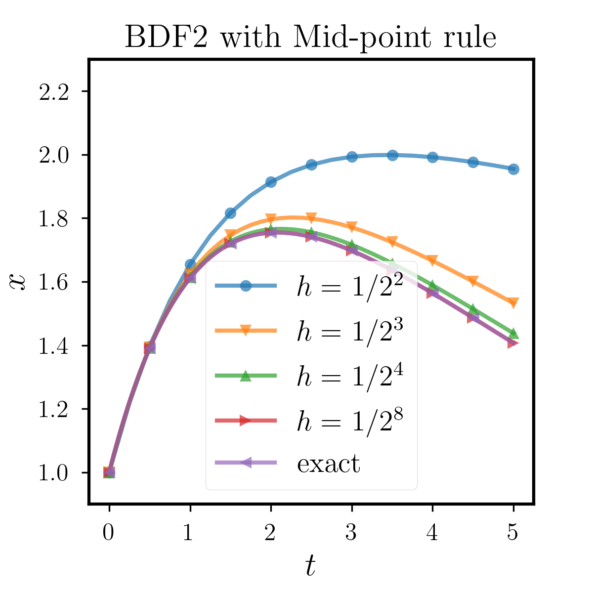
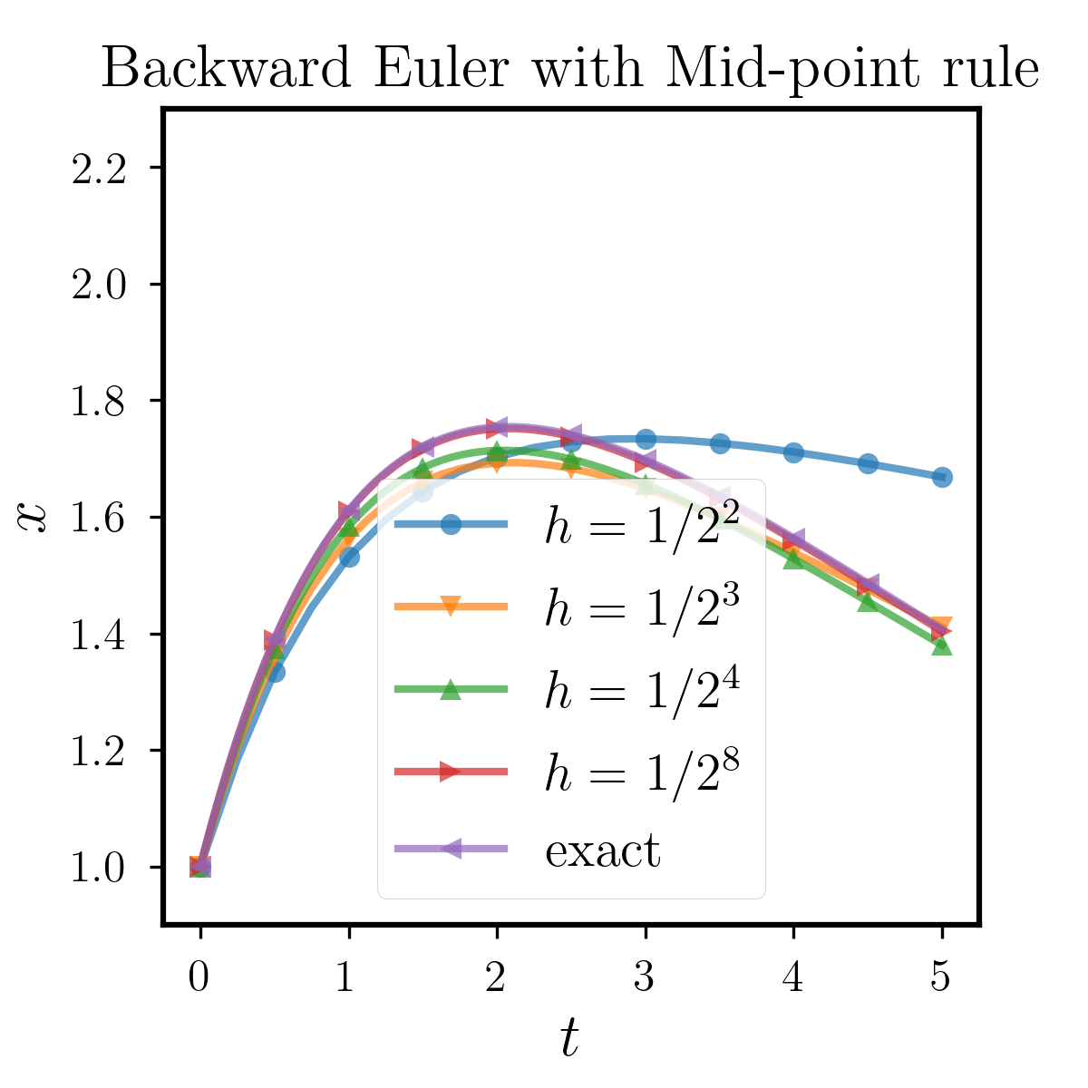
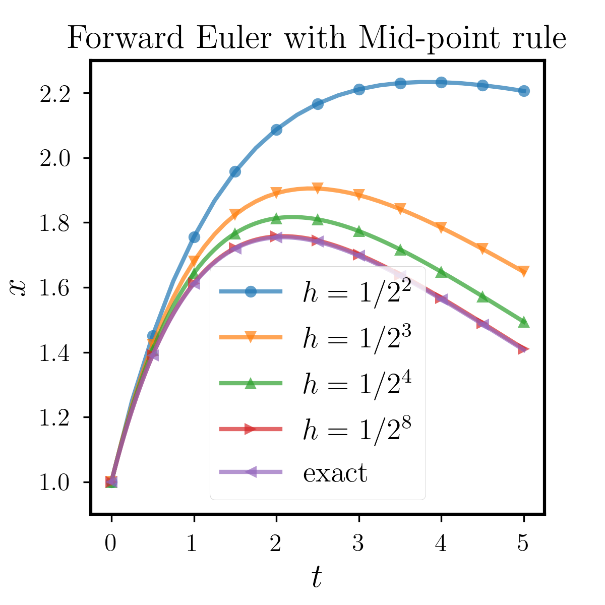
Firstly we perform numerical experiments to verify the zero-stability that we have proved above. As we have Theorem 2 that all the classical LMMs that satisfy the root condition are zero-stable after being equipped with open quadrature. In this subsection, we consider the most commonly used methods, i.e., Forward Euler, Backward Euler and BDF2 that are all zero-stable in our conclusion. We vary the time step from $h=1/2^{2}$ to $h=1/2^{8}$ , and observe the performance of the numerical solutions.

6.1.1 Example 1

We consider the following ODE with memory:

\dot{x}(t)=x(t)-\int_{0}^{t}2\text{e}^{-1.9(t-s)}x(s)\,\mathop{}\!\mathrm{d}s,\quad x(0)=1.

(6.1)

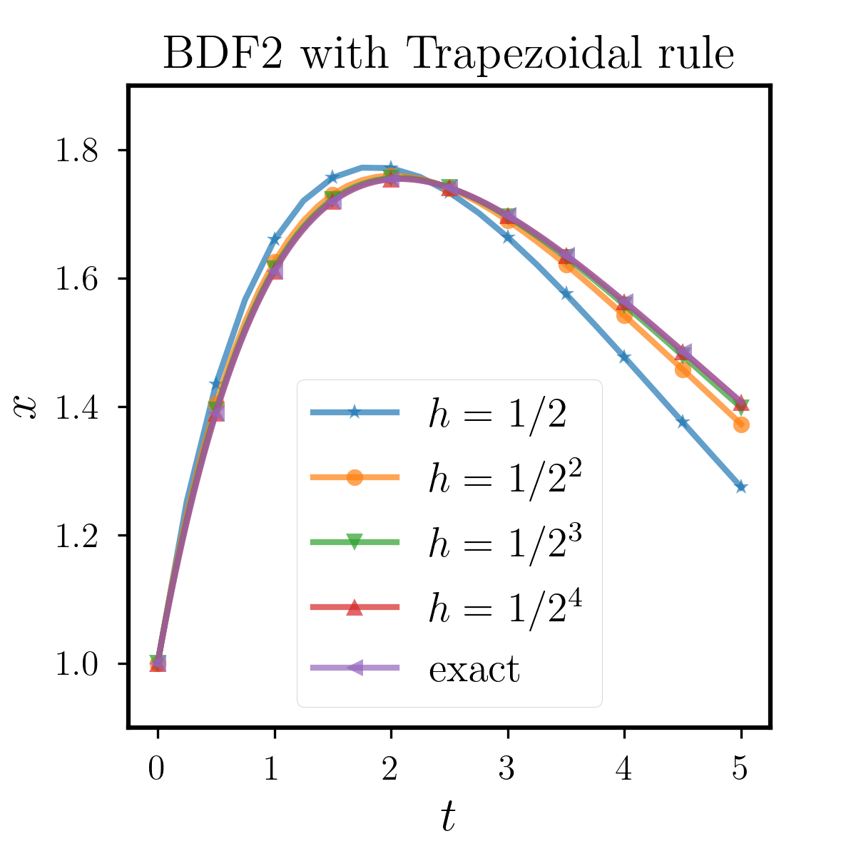
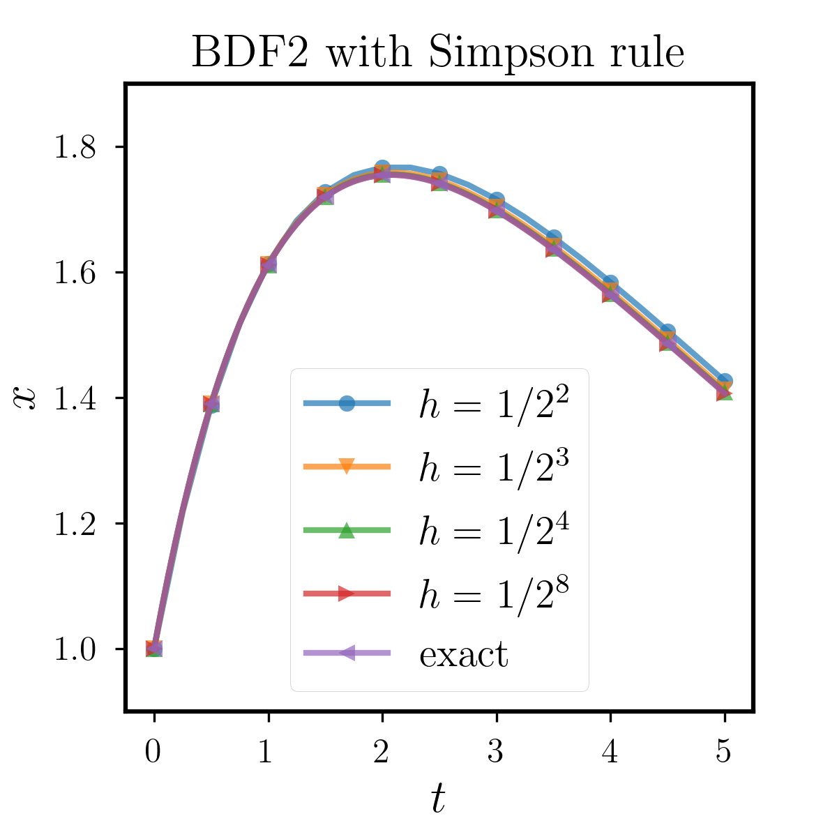
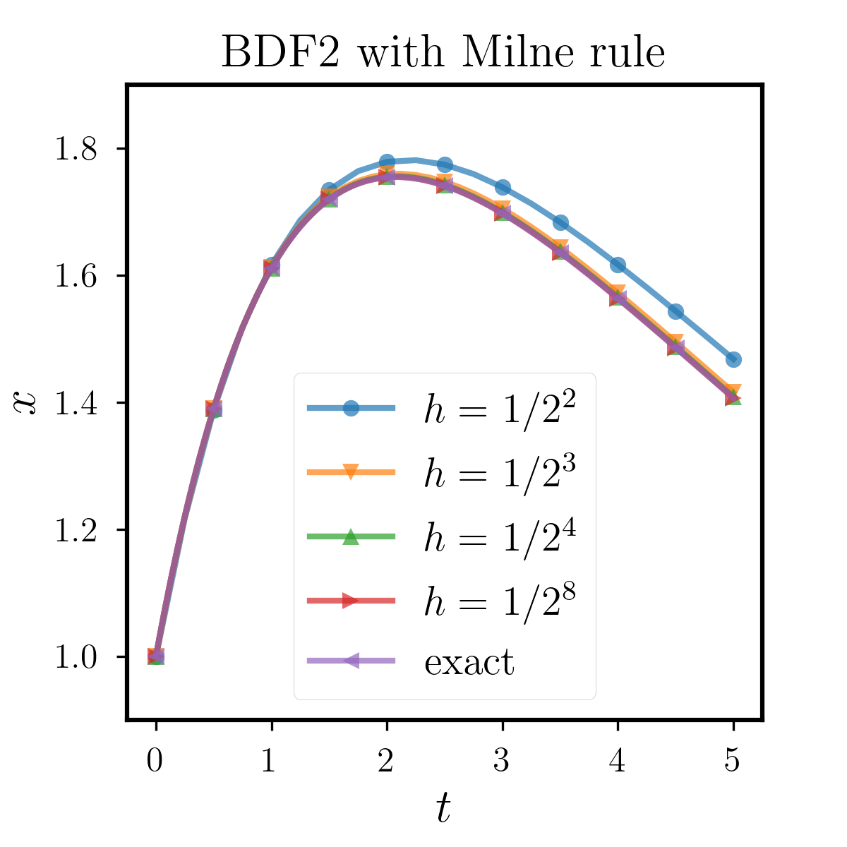
We can see that the memory item in this example is an exponential function, thus we can obtain the exact soluiton of the equation through Laplace Transform. We first fix the quadrature as open Mid-point rule, and compare the stability between BDF2, Backward Euler and Forward Euler methods. The results are shown in Figure 6.1.1, where we can observe that when the step size $h$ is relatively small, the three methods can approximate the true solution well. However, as we increase $h$ , different methods have errors due to accuracy issues. With the same quadrature as Mid-point rule, the performance of the Forward Euler is relatively poor, while that of the Backward Euler and BDF2 are similarly better. Moreover, to study the effects of different quadratures, we test BDF2 with Trapezoidal rule, Simpson rule and Milne rule. All of them have higher order than Mid-point rule and the results are shown in Figure 6.1.2. We can see that all the methods perform better than that with Mid-point rule as we expect. From this example, we conclude that these two implicit methods have superior numerical performance than the explicit Forward Euler. As for the usage of quadratures, the above tests show that the stable domain highly depends on the quadrature rules we use, which should be carefully chosen in applications.

Refer to caption — Figure 6.1.1: Performance of different methods with the same quadrature. From the left to the right, we apply BDF2, Backward Euler and Forward Euler with Mid-point rule to (6.1). The time steps $h=1/2^{2},1/2^{3},1/2^{4},1/2^{8}$ , the $5$ solid curves represent numerical solution of different $h$ and exact solution which is obtained by Laplace Transform.

6.1.2 Example 2

In the previous example, we consider an exponential memory term, which has a relatively weak impact on the solution. In this example, we change the kernel to a power function then the equation reads:

\dot{x}(t)=x(t)-\int_{0}^{t}\frac{10}{(t-s+1)^{2}}\mathop{}\!\mathrm{d}s,\quad x(0)=1.

(6.2)

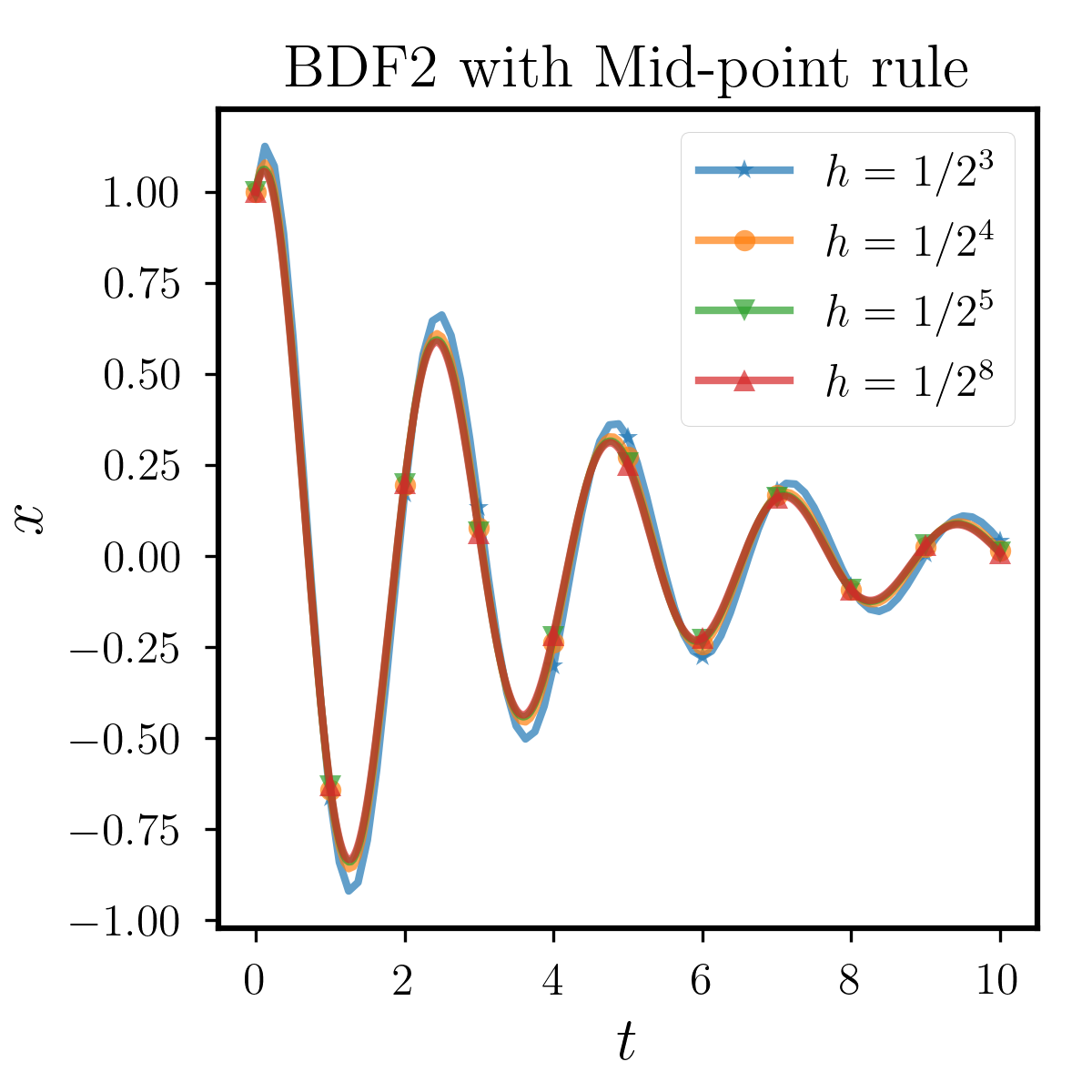
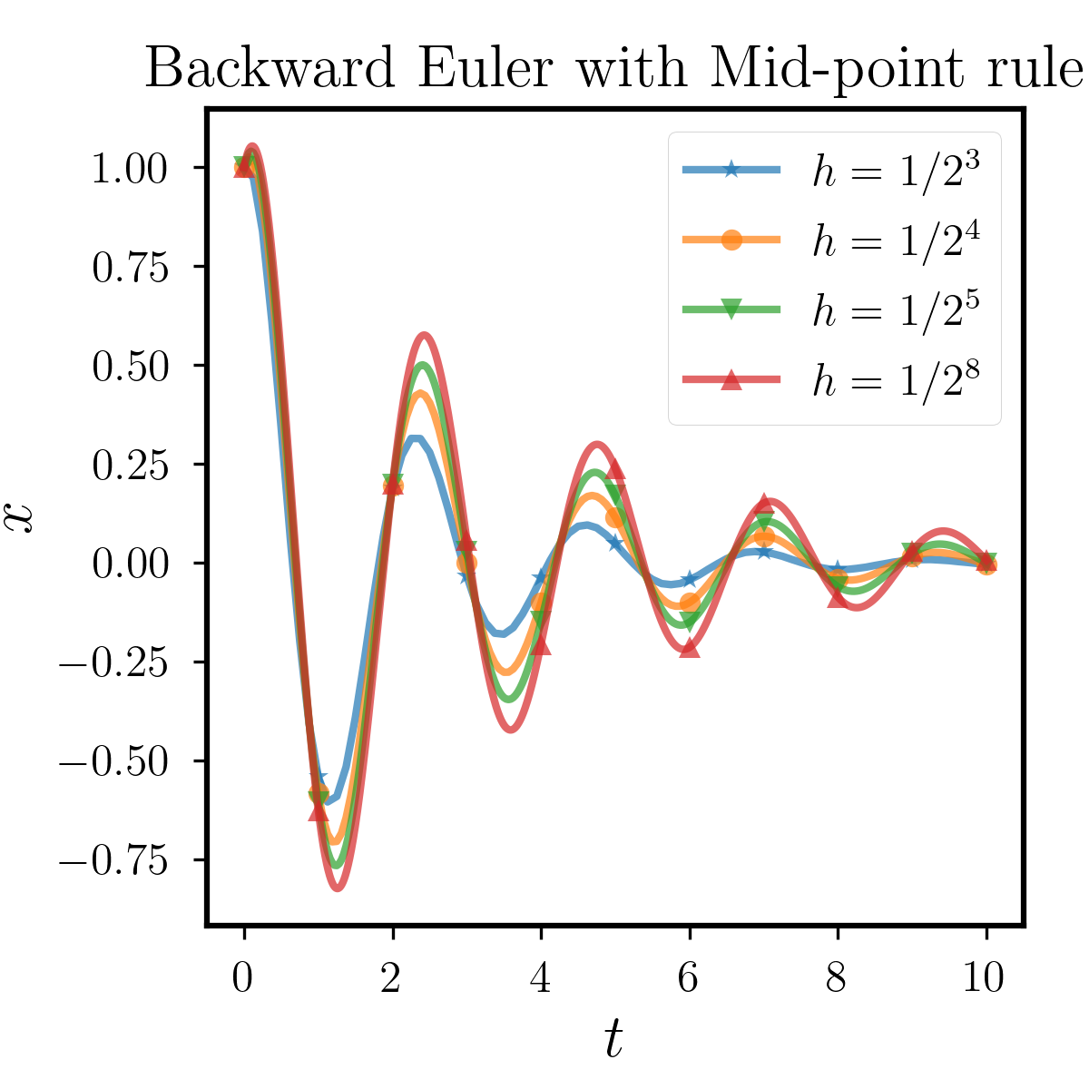
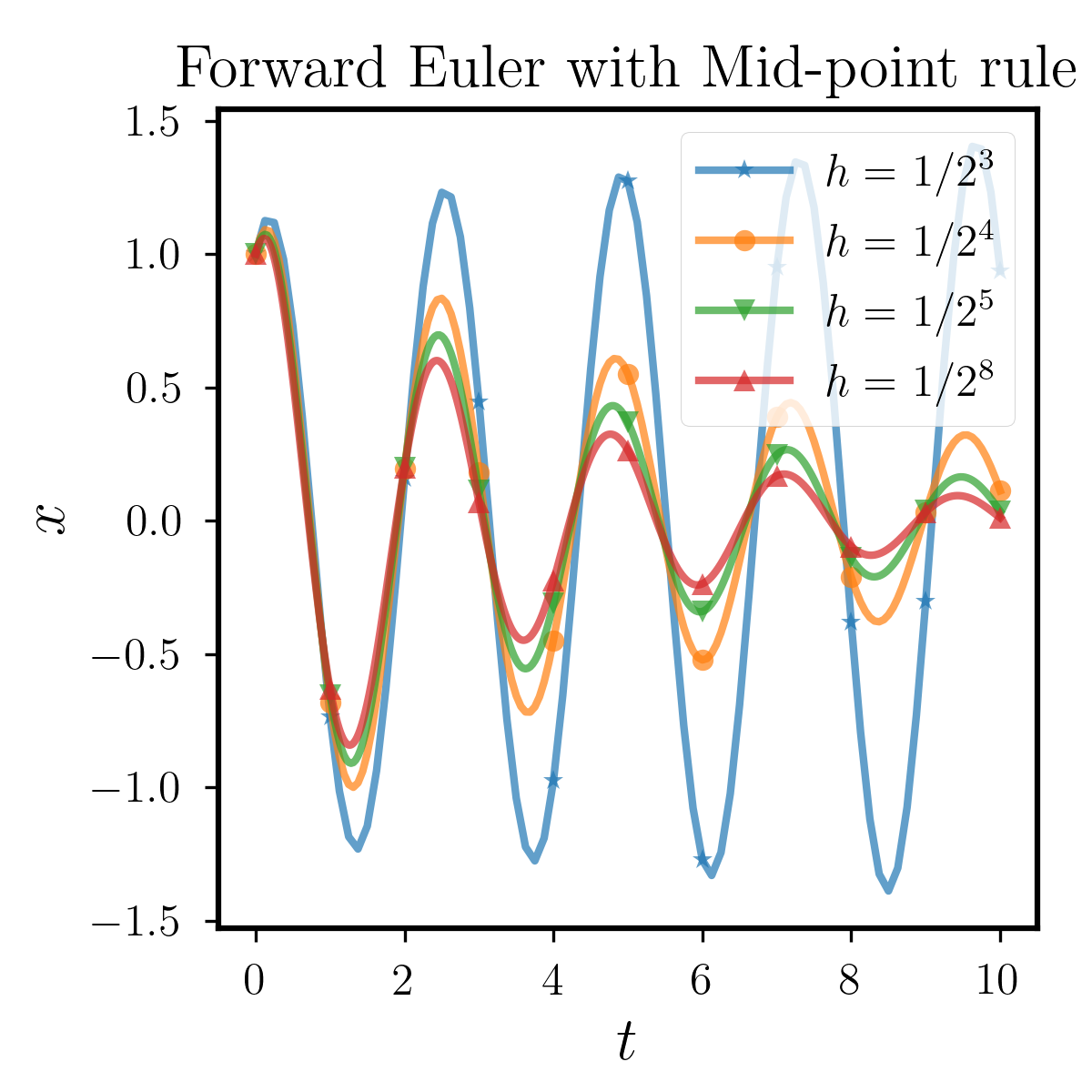
At this time, we can not derive the analytic solution so that we treat the numerical solution with $h=1/2^{8}$ as the exact solution. The result are shown in Figure 6.1.3, where we observe that the solution of the (6.2) is periodically oscillatory and decaying. In this example, we still use the Mid-point rule to compare the differences between the three different multi-step methods. It can be seen that for various step sizes, the BDF2 can capture this periodic oscillation well, while for the two Euler methods, as the step size is relatively larger, the numerical solution has a significantly higher or lower amplitude. Therefore, BDF2 has a clear advantage over the two Euler methods in this example.

6.2 Convergence

In this subsection, we test the convergence of the proposed methods for ODEs with memory. In the following examples, we set various time steps and measure the error of the numerical solutions. We use the following error measure:

\text{error}:=\lVert x(t)-x_{\text{exact}}(t)\rVert_{\infty}=\max_{t_{i}\in[0,T]}\left\lvert x(t_{i})-x_{\text{exact}}(t_{i})\right\rvert,

(6.3)

where the exact solution $x_{\text{exact}}(t)$ is obtained analytically and $t_{i}$ is a grid point. As we have Lemma 2, the order of LMM is determined by both the classical LMM and the quadrature. Thus we will combine different method with different quadratures and verify the order of the error we define as (6.3).

6.2.1 Example 3

In this example we consider the equation

\dot{x}(t)=x(t)-\int_{0}^{t}2\text{e}^{-(t-s)}x(s)\mathop{}\!\mathrm{d}s,\quad x(0)=1.

(6.4)

This equation has an analytical solution:

x(t)=\sin(t)+\cos(t).

(6.5)

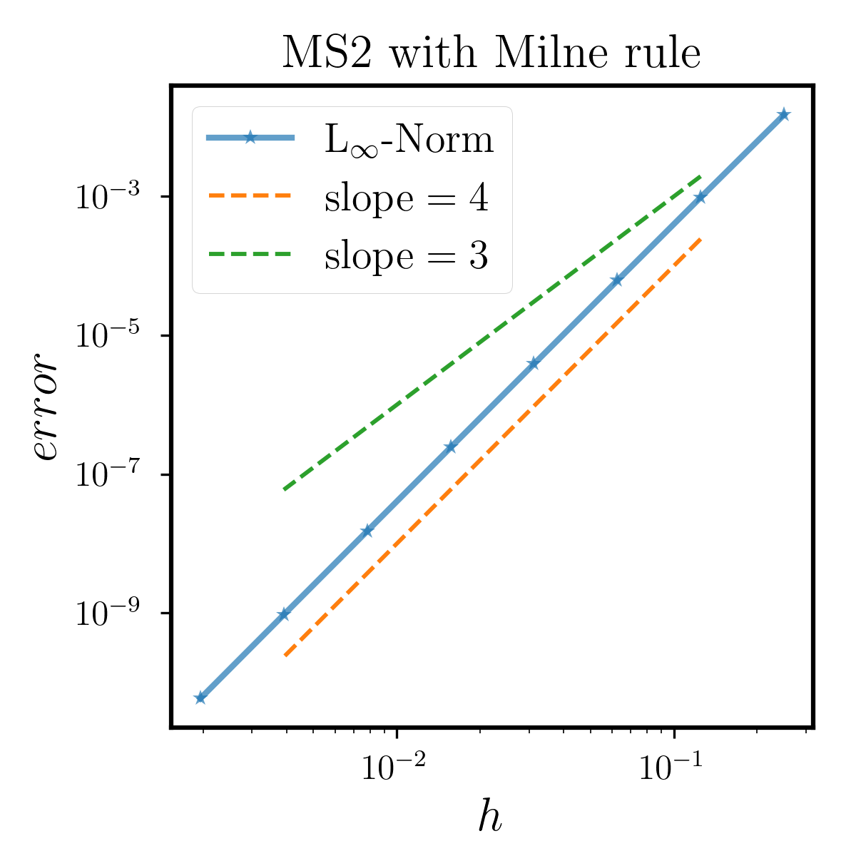
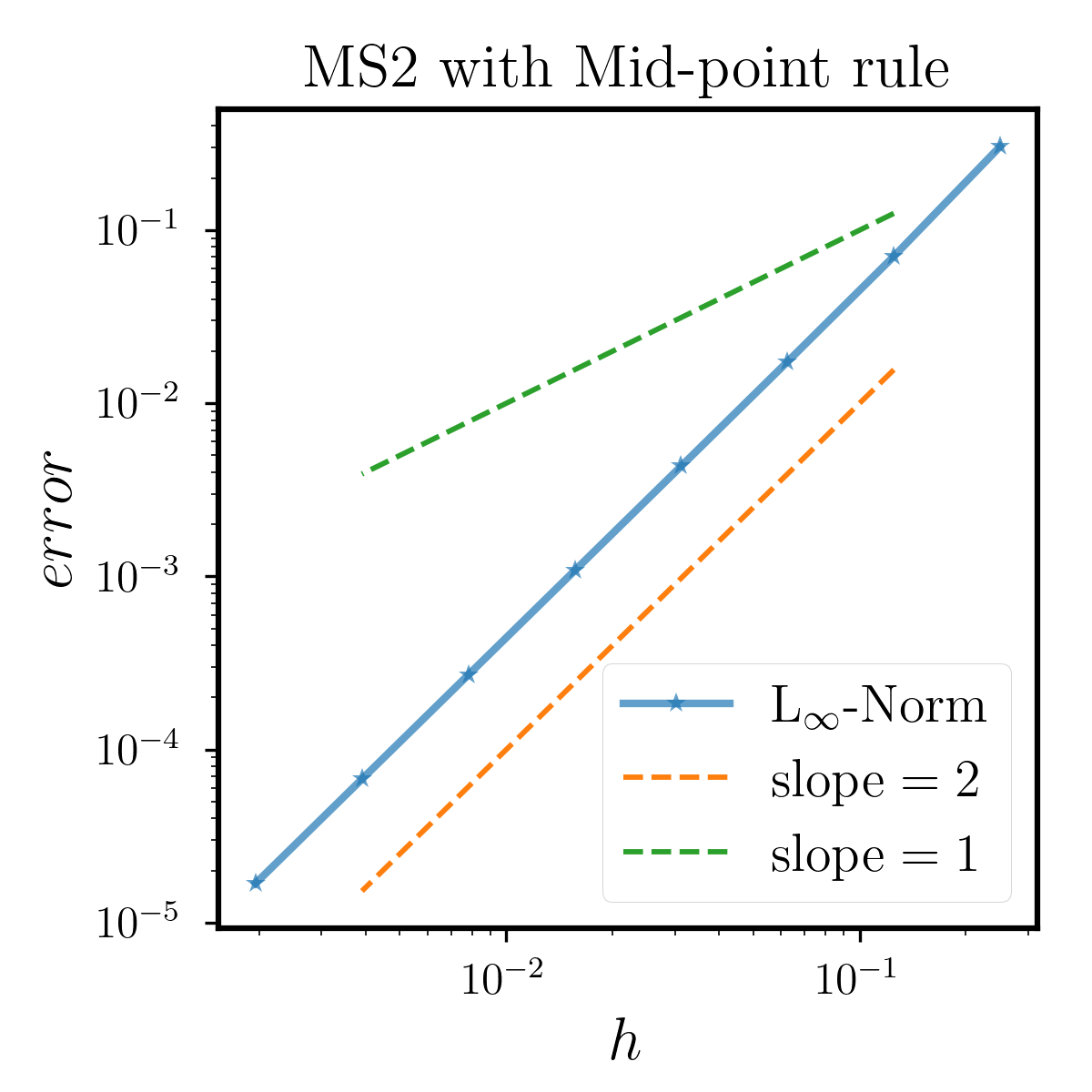
We test MS2 with both Milne rule and Mid-point rule for convergence from $t=0$ to $t=10$ . Recall that MS2 is a fourth-order method, the order of composed Milne rule and composed Mid-point rule is $4$ and $2$ . The results are shown in Figure 6.2.1, where both the $x$ -axis and $y$ -axis are on a logarithmic scale. It shows that MS2 with Milne rule is fourth-order accurate as the order of both two components are $4$ . While MS2 with Mid-point rule is second-order accurate, since it is restricted by the accuracy of quadrature.

6.2.2 Example 4

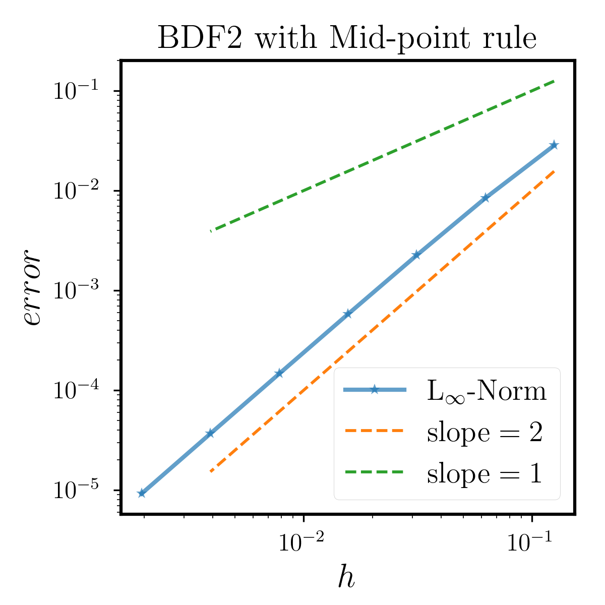
In this example, we change the memory kernel and use BDF2 instead to solve the equation which reads

\dot{x}(t)=-x(t)+\int_{0}^{t}8\text{e}^{-3(t-s)}x(s)\mathop{}\!\mathrm{d}s,\quad x(0)=1.

(6.6)

The analytical solution is

x(t)=\left(\frac{1}{3}\sinh(3t)+\cosh(3t)\right)\text{e}^{-2t}.

(6.7)

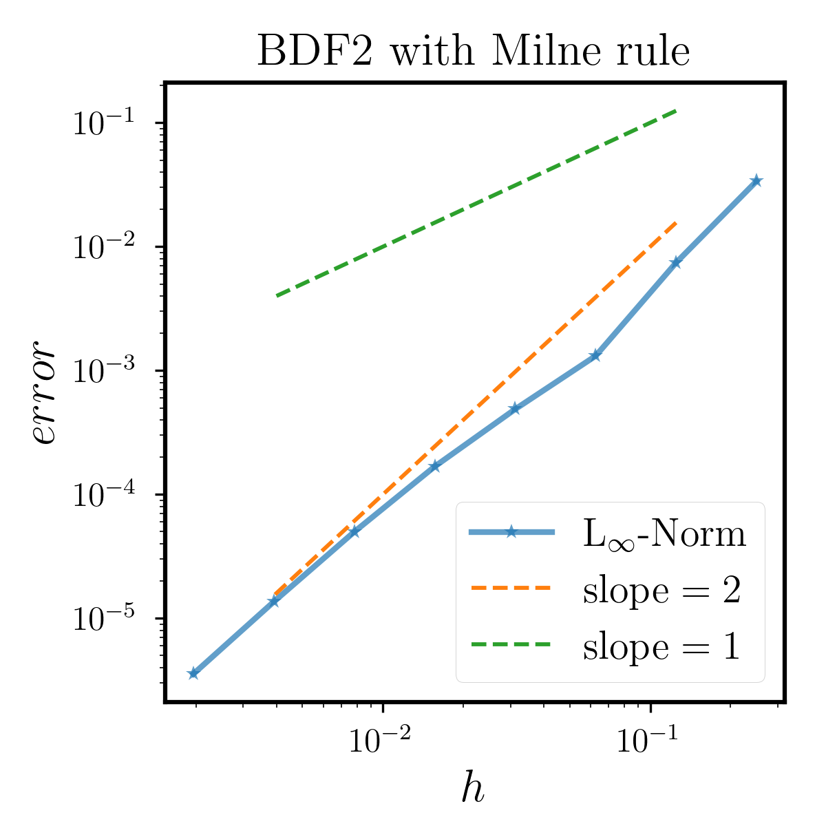
We test the convergence rate of BDF2 with both Milne rule and Mid-point rule from $t=0$ to $t=5$ . The results are shown in Figure 6.2.2, which shows that both methods are second-order accurate. Unlike the former example, the two methods are mainly restricted by the accuracy of the BDF2, as it is just of order $2$ .

From the above two examples, we can see that the order of the method is determined by both the classical LMM and the quadrature rule, i.e., when we use MS2 the error of integral part is dominant. From this prospective, it is unnecessary to use a method with a large difference of order between the two components.

6.3 Weak A-stability

Finally, we verify the weak A-stability results proved in Section 5, where we give the modified definition 11 and obtain that Backward Euler is weak A-stable.

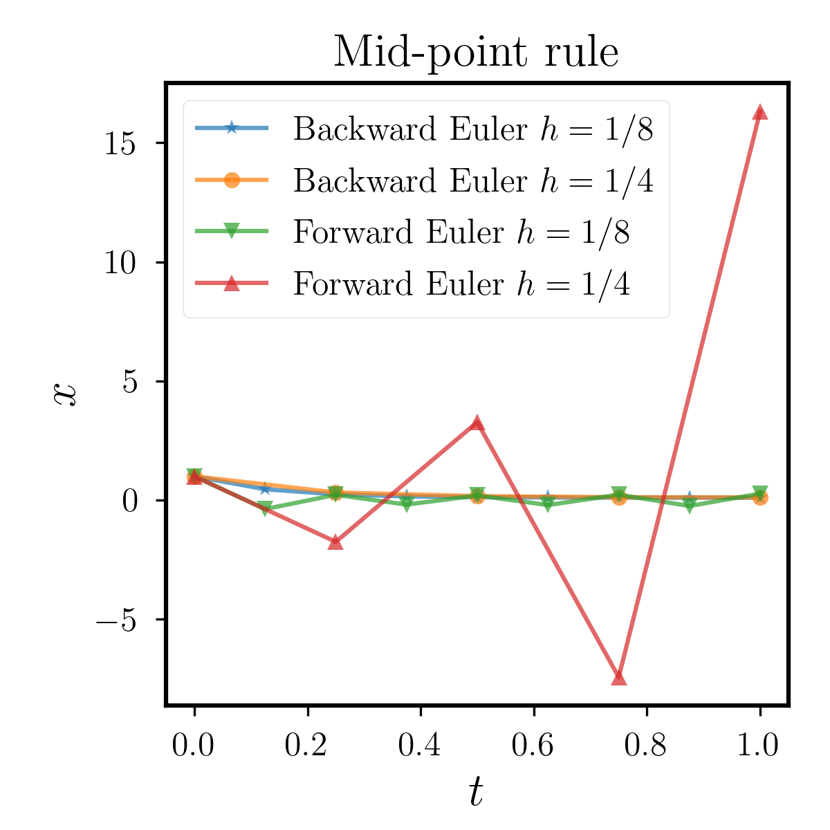
6.3.1 Example 5

In this example, we can consider the equation

\dot{x}=-11x+\int_{0}^{t}10\text{e}^{-(t-s)}x(s)\mathop{}\!\mathrm{d}s,\quad x(0)=1.

(6.8)

Here $\lambda=-11$ , $\kappa=10$ , thus $\lambda+\kappa<0$ and the solution of (6.8) is absolutely stable. Numerically, we use Mid-point as the quadrature, with $h$ values of $1/4$ and $1/8$ , and employ the Forward Euler method and the Backward Euler method. The results are shown in the left side of Figure 6.3.1. It is observed that the numerical solutions obtained from the Backward Euler method, which is weak A-stable, are stable for both $h$ . While for the Forward Euler method, the numerical solution obtained with a larger $h$ , i.e., $h=1/4$ is divergent, indicating that the method is not weak A-stable.

6.3.2 Example 6

In this example, we discuss our modified definition weak A-stability, where the “weakness” results from that we treat (5.9) as the region of absolute stability for the exact solution which should be a proper subset of the region. However, as we can derive the analytic solution when the kernel is exponential. We find that $\left\{(\lambda,k(\cdot)):\lambda+\int_{0}^{\infty}\left\lvert k(\xi)\right\rvert\mathop{}\!\mathrm{d}\xi<0\right\}$ indeed equals to $\mathcal{R}_{\text{exact}}$ in the case of exponential kernel. In this example, we consider the power function kernel and study the distinction of the two sets in (5.9). We look at the following equation:

\dot{x}(t)=\lambda x+\int_{0}^{t}\frac{10}{{(t-s+1)}^{2}}x(s)\mathop{}\!\mathrm{d}s,\quad x(0)=1,

(6.9)

with $\lambda+\kappa=-10+10=0$ or $\lambda+\kappa=-10.1+10=-0.1$ .

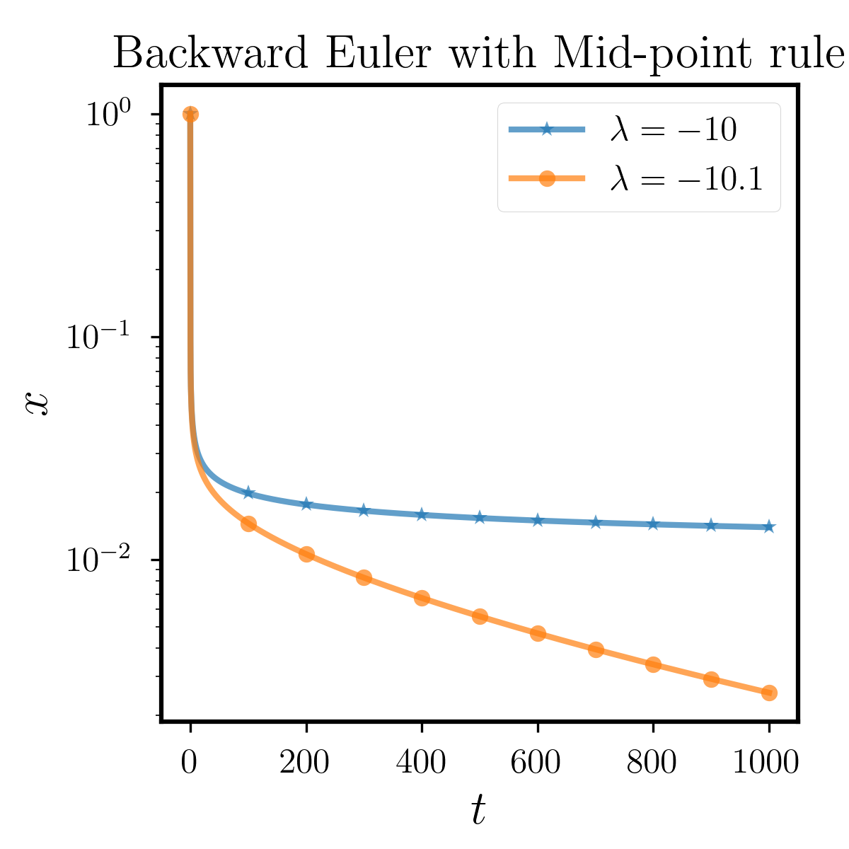
In this experiment, we use Backward Euler with Mid-point rule and set $h=1/2^{8}$ so that we treat the solution as exact one. The results are shown in the right side of Figure 6.3.1. It can be observed that we take the logarithmic scale on the $y$ -axis to observe the changes in the function value. When $\lambda+\kappa=0$ , we found that solution value is convergent at a non-zero value, indicating that this setting does not belong to the absolute stability region $\mathcal{R}_{\text{exact}}$ . However, when $\lambda+\kappa=-0.1$ , we can see that the solution continues to monotonically decrease. We calculate its long-term behavior up to $t=1000$ and conclude that it converges to zero, although it does so slowly, indicating that this setting is within $\mathcal{R}_{\text{exact}}$ . These phenomena show that numerically $\left\{(\lambda,k(\cdot)):\lambda+\int_{0}^{\infty}\left\lvert k(\xi)\right\rvert\mathop{}\!\mathrm{d}\xi<0\right\}$ equals to $\mathcal{R}_{\text{exact}}$ when we use the type of kernel in (6.9). From this point of view, our modified definition is properly reasonable for at least some types of kernel function.

References

[1] O. Arino, M. L. Hbid, and E. A. Dads, Delay Differential Equations and Applications: Proceedings of the NATO Advanced Study Institute held in Marrakech, Morocco, 9-21 September 2002, vol. 205, Springer Science & Business Media, 2007.
[2] V. I. Arnold, Ordinary Differential Equations, 10th printing, 1998.
[3] R. E. Bellman and K. L. Cooke, Differential-difference Equations, Rand Corporation, 1963.
[4] R. L. Burden and D. J. Faires, Numerical Analysis, PWS publishing company, 1985.
[5] P. J. Davis and P. Rabinowitz, Methods of Numerical Integration, Courier Corporation, 2007.
[6] D. F. Griffiths and D. J. Higham, Numerical Methods for Ordinary Differential Equations: Initial Value Problems, Springer Science & Business Media, 2010.
[7] E. Hairer, S. P. Nørsett, and G. Wanner, Solving Ordinary Differential Equations I: Nonstiff Problems, Springer-Verlag, 1987.
[8] R. Hilfer, Applications of fractional calculus in physics, World scientific, 2000.
[9] H.-l. Liao, D. Li, and J. Zhang, Sharp error estimate of the nonuniform l1 formula for linear reaction-subdiffusion equations, SIAM Journal on Numerical Analysis, 56 (2018), pp. 1112–1133.
[10] H.-L. Liao, W. McLean, and J. Zhang, A second-order scheme with nonuniform time steps for a linear reaction-sudiffusion problem, arXiv preprint arXiv:1803.09873, (2018).
[11] H.-l. Liao, W. McLean, and J. Zhang, A discrete gronwall inequality with applications to numerical schemes for subdiffusion problems, SIAM Journal on Numerical Analysis, 57 (2019), pp. 218–237.
[12] P. Linz, Analytical and numerical methods for Volterra equations, SIAM, 1985.
[13] N. Liu, H. Qin, and Y. Yang, Unconditionally optimal h1-norm error estimates of a fast and linearized galerkin method for nonlinear subdiffusion equations, Computers & Mathematics with Applications, 107 (2022), pp. 70–81.
[14] I. Podlubny, An introduction to fractional derivatives, fractional differential equations, to methods of their solution and some of their applications, Math. Sci. Eng, 198 (1999), p. 340.
[15] J. L. Schiff, The Laplace transform: theory and applications, Springer Science & Business Media, 1999.
[16] H. Smith, An introduction to delay differential equations with applications to the life sciences, springer, 2011.
[17] M. R. Spiegel, Laplace transforms, McGraw-Hill New York, 1965.
[18] J. Stoer and R. Bulirsch, Introduction to Numerical Analysis, vol. 12, Springer Science & Business Media, 2013.
[19] L. Torelli, Stability of numerical methods for delay differential equations, Journal of Computational and Applied Mathematics, 25 (1989), pp. 15–26.
[20] W.-S. Wang, S.-F. Li, and K. Su, Nonlinear stability of general linear methods for neutral delay differential equations, Journal of Computational and Applied Mathematics, 224 (2009), pp. 592–601.
[21] G. Wanner and E. Hairer, Solving Ordinary Differential Equations II: Stiff and Differential-Algebraic Problems, Springer Berlin Heidelberg, 1996.