NVC-1B: A Large Neural Video Coding Model
Abstract
The emerging large models have achieved notable progress in the fields of natural language processing and computer vision. However, large models for neural video coding are still unexplored. In this paper, we try to explore how to build a large neural video coding model. Based on a small baseline model, we gradually scale up the model sizes of its different coding parts, including the motion encoder-decoder, motion entropy model, contextual encoder-decoder, contextual entropy model, and temporal context mining module, and analyze the influence of model sizes on video compression performance. Then, we explore to use different architectures, including CNN, mixed CNN-Transformer, and Transformer architectures, to implement the neural video coding model and analyze the influence of model architectures on video compression performance. Based on our exploration results, we design the first neural video coding model with more than 1 billion parameters—NVC-1B. Experimental results show that our proposed large model achieves a significant video compression performance improvement over the small baseline model, and represents the state-of-the-art compression efficiency. We anticipate large models may bring up the video coding technologies to the next level.
Index Terms:
Neural Video Coding, Large Model, Motion Coding, Contextual Coding, Temporal Context Mining.I Introduction
The popularity of video applications, such as short video-sharing platforms, video conferences, and streaming television, has made the amount of video data increase rapidly. The large data amount brings large costs for video transmission and storage. Therefore, it is urgent to compress videos efficiently to reduce video data amount.
To decrease the costs of video transmission and storage, various advanced coding technologies have been proposed, including intra/inter-frame prediction, transform, quantization, entropy coding, and loop filters. These coding technologies have led to the development of a series of video coding standards over the past decades, such as H.264/AVC [1], H.265/HEVC [2], and H.266/VVC [3]. These video coding standards have significantly improved video compression performance.
Although traditional video coding standards have achieved great success, their compression performance is increasing at a slower speed than that of video data amount. To break through the bottleneck of video compression performance growth, researchers have begun to explore end-to-end neural video coding in recent years. Existing end-to-end neural video coding (NVC) models can be roughly classified into four classes: volume coding-based [4, 5], conditional entropy modeling-based [6, 7], implicit neural representation-based [8, 9, 10, 11], motion compensated prediction-based [12, 13, 14, 15, 16, 17, 18, 19, 20, 21, 22, 23, 24, 25, 26, 27, 28, 29, 30, 31, 32, 33, 34, 35, 36, 37, 38, 39]. With the development of neural networks in the fields of natural language processing and computer vision, recent neural video coding models [32, 39, 40] have surpassed the reference software of H.266/VVC standard under certain coding conditions. However, the development speed of neural video coding is lower than that of natural language processing and computer vision. One typical example is that the emerging large models for natural language processing or computer vision have achieved great success, but large models for neural video coding are still unexplored.
Large models for natural language processing and computer vision have attracted much attention recently. Large language models (LLMs) and large vision models (LVMs) are commonly first built on small models and then their model sizes are gradually scaled up. Following the scaling law [41], increasing the model sizes can bring impressive task performance gains. In terms of LLMs, their model sizes can reach hundreds to thousands of billion (B). For example, the representative LLMs—GPT-3 [42] and GPT-4 [43] developed by OpenAI contain 175B parameters and 1800B parameters, respectively. Their natural language understanding ability and human language generation ability are greatly improved. In terms of LVMs, their model sizes are much smaller than those of LLMs. For example, the Segment Anything Model (SAM) [44] used for image segmentation and the Depth Anything Model [45] only contain 636 million (M) parameters and 335M parameters. Even the largest Vision Transformer (ViT) [46] models have only recently grown from a few hundred million to 22B [47]. Although the model sizes of current LVMs are much smaller than those of LLMs, larger model sizes for vision models still greatly improve computer vision task performance [48].
Witnessing the success of LLMs and LVMs, in this paper, we try to explore the effectiveness of large model for neural video coding. We regard a small model–DCVC-SDD [32] as our baseline, which is based on the typical conditional coding architecture [34, 30, 35, 39] and has a higher compression performance than the reference software of H.266/VVC—VTM-13.0 [49] under certain testing conditions. We first analyze the influence of model sizes on compression performance. Specifically, we gradually scale up the model sizes of its motion encoder-decoder, motion entropy model, contextual encoder-decoder, contextual entropy model, and temporal context mining module. Then, we analyze the influence of model architectures on compression performance. Specifically, we try to replace the CNN architecture with mixed CNN-Transformer or Transformer-only architecture. Finally, we build a large neural video coding model with 1B parameters—NVC-1B.
Our contributions are summarized as follows:
-
•
We scale up the model sizes of different parts of a neural video coding model and analyze the influence of model sizes on video compression performance.
-
•
We use different architectures to implement the neural video coding model and analyze the influence of model architectures on video compression performance.
-
•
Based on our exploration results, we propose the first large neural video coding model with more than 1B parameters—NVC-1B and achieve a significant video compression performance gain over the small baseline model.
The remainder of this paper is organized as follows. Section II gives a review of related work about LLM, LVM, and neural video coding. Section III introduces the framework overview of our proposed NVC-1B. Section IV analyzes the influence of model sizes and model architectures on compression performance in detail. Section V reports the compression performance of NVC-1B and gives some analyses. Section VI gives a conclusion of this paper.
II Related Work
II-A Large Language Model
A large language model (LLM) refers to a language model containing billions of parameters with the goal of natural language understanding and human language generation. Recently, a variety of LLMs have emerged, including those developed by OpenAI (GPT-3 [42] and GPT-4 [43]), Google (GLaM [50], PaLM [51], PaLM-2 [52], and Gemini [53]), and Meta (LLaMA-1 [54], LLaMA-2 [54], and LLaMA-3 [55]). These models are commonly first built upon the small language models. Then, under the guidance of the scaling law [41], they largely scale the model sizes. For example, GPT-3 contains 175B parameters and GPT-4 even contains 1800B parameters. Owing to the massive scale in model sizes, LLMs have achieved significant performance across various tasks. They can better understand natural languages and generate high-quality texts based on interactive contexts, such as prompts.
II-B Large Vision Model
The success of LLMs leads to the rise of large vision models (LVMs). Similar to LLMs, scaling up the model sizes of small vision models has also shown improved performance for various tasks. Google researchers [47] proposed Vision Transformer (ViT) [46] for image and video modeling. Its model sizes gradually increase from several hundred million to 4B [56]. Recently, its model size has even been extended to 22B [47] and achieved the current state-of-the-art ranging from (few-shot) classification to dense output vision tasks. Based on the ViT backbone, LAION researchers [57] have investigated scaling laws for contrastive language-image pre-training (CLIP) [58]. The largest model based on ViT-G/14 can reach 1.8B parameters. Their investigation shows that scaling up the model size of CLIP can improve the performance of zero-shot classification of downstream vision tasks. Also based on ViT, Meta researchers proposed a Segment Anything Model (SAM) [44] for image segmentation. The largest SAM model has about 636M parameters and has achieved excellent segmentation accuracy on many benchmark datasets. Tiktok researchers proposed a Depth Anything Model [45] with 335M parameters for monocular image depth estimation and has shown impressive depth estimation accuracy. Although the model sizes of current LVMs are much smaller than those of LLMs, these pioneering works of LVMs still verify the benefits of scaling up the model sizes for visual tasks. However, no research has explored the effectiveness of scaling up the model size of neural video coding models.
II-C Neural Video Coding
Neural video coding [37, 4, 59, 19, 60, 25, 14, 12, 23, 6, 17, 15, 16, 24, 13, 8, 34, 21, 61, 62, 63, 7, 64, 26, 29, 27, 65, 28, 9, 66, 30, 40, 67, 68, 33, 69, 11] has explored a new direction for video compression in recent years. Among different kinds of coding schemes, motion compensation-based schemes have achieved state-of-the-art compression performance.
DVC [60] is a pioneering scheme of motion compensation-based neural video coding. It follows the traditional hybrid video coding framework but implements main modules with neural networks, such as motion estimation, motion compression, motion compensation, residual compression, and entropy models. Based on DVC, subsequent schemes mainly focus on how to increase the accuracy of temporal prediction. For example, Lin et al. [15] proposed M-LVC that introduces multiple reference frames for motion compensation and motion vector prediction. Agustsson et al. [17] proposed SSF that generalizes typical motion vectors to a scale-space flow for better handling complex motion. Hu et al. [16] proposed FVC that shifts temporal prediction from pixel domain to feature domain using deformable convolution [70].
Different from DVC-based schemes, DCVC [34] shifts the typical residual coding paradigm to a conditional coding paradigm. Regarding temporal prediction as a condition, DCVC feeds the condition into a contextual encoder-decoder, allowing the networks to learn how to reduce temporal redundancy automatically rather than performing explicit subtraction operations. Based on DCVC, Sheng et al. [30] proposed DCVC-TCM that designs a temporal context mining module to generate multi-scale temporal contexts. This work greatly improved the compression performance of neural video coding and began to make fair comparisons with standard reference software of traditional codecs. Following DCVC-TCM, DCVC-HEM [35], DCVC-DC [39], and DCVC-SDD [32] were further proposed. They focus on introducing more temporal conditions to utilize temporal correlation, such as latent-prior, decoding parallel-friendly spatial-prior, and long-term temporal prior. Nowadays, the compression performance of the DCVC series has exceeded that of the reference software of H.266/VVC [71].
Existing neural video coding models commonly have small model sizes. In this work, we try to scale up the model size of a neural video coding model to explore the influence of model size on video compression performance.
III Overview
We build the large neural video coding model–NVC-1B based on our small baseline model DCVC-SDD [32]. We first give a brief overview of the framework of our NVC-1B.
III-1 Motion Estimation
Similar to our small baseline model DCVC-SDD, we use the structure and detail decomposition-based motion estimation method to estimate the motion vectors between adjacent video frames [32]. Specifically, we first decompose the current frame and the reference frame into structure components (, ) and detail components (, ) . Then, we estimate the motion vectors (, ) of the structure and detail components respectively using a pre-trained SpyNet [72].
III-2 Motion Encoder-Decoder
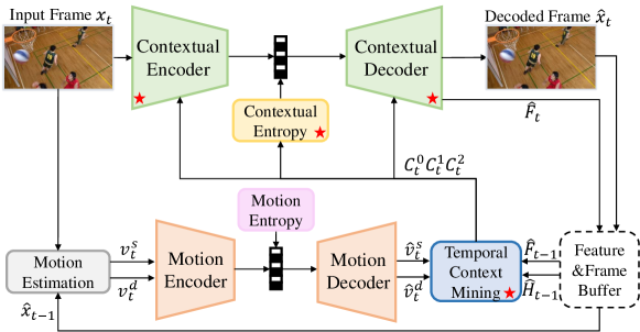
We use an autoencoder-based motion encoder-decoder to compress and reconstruct the estimated motion vectors (MVs) jointly, as shown in Fig. 1. Specifically, we first perform channel-wise concatenation to the input motion vectors and . Then, the MV encoder compresses them into a compact latent representation with the size of . is the height and is the width of the input motion maps. is the number of channels of the compact latent representation . After quantization, the quantized latent representation is signaled into a bitstream using the arithmetic encoder. After receiving the transmitted bitstream, the arithmetic decoder reconstructs the bitstream back to the quantized latent representation . The MV decoder then decompresses back to the reconstructed motion vectors and .
III-3 Temporal Context Mining
The temporal context mining module is essential for conditional-based neural video coding schemes [32, 33, 30, 37, 34, 35, 39, 40]. Given a reference feature , the temporal context mining module first uses a feature pyramid to extract multi-scale features from . Then, it uses muli-scale motion vectors to perform feature-based motion compensation to these features and learn multi-scale temporal contexts ,,. To handle motion occlusion, following our baseline [32], we use a ConvLSTM-based long-term reference generator to accumulate the historical information of each reference feature and learn a long-term reference feature . Then, we fuse with ,, to generate long short-term fused temporal contexts ,,.
III-4 Contextual Encoder-Decoder
We use an autoencoder-based contextual encoder and decoder to compress and reconstruct the input frame . The contextual encoder compresses into a compact latent representation with the size of . is the number of channels of the compact latent representation . In the encoding procedure, multi-scale temporal contexts ,, learned by the temporal context mining module are channel-wise concatenated into the contextual encoder to reduce temporal redundancy. Then, quantization is performed to and the arithmetic encoder converts the quantized latent representation to a bitstream. After receiving the transmitted bitstream, the arithmetic decoder reconstructs it to . The contextual decoder decompresses to a reconstructed frame . In the decoding procedure, the multi-scale temporal contexts ,, are also concatenated into the contextual decoder. Before obtaining , an intermediate feature of the contextual decoder with the size of is regarded as the reference feature for encoding/decoding the next frame.
III-5 Entropy Model
We use the factorized entropy model [73] for hyperprior and the Laplace distribution [74] to model the motion and contextual compact latent representations and . When estimating the mean and scale of the Laplace distribution of and , we combine the hyperprior, latent prior, and the spatial prior generated by the quadtree partition-based spatial entropy model [32, 39] together. For , we also introduce a temporal prior learned from the smallest-resolution temporal context .
IV Methodology
To explore the influence of model size on compression performance, we gradually scale up the model sizes of different parts of our small neural video coding model [32], including its motion encoder-decoder, motion entropy model, contextual encoder-decoder, contextual entropy model, and temporal context mining module. Since most existing neural video coding models use a pre-trained optical flow model for motion estimation and focus on designing other coding parts, we do not scale up the model size of the motion estimation module in this work. To explore the influence of model architecture on compression performance, we use different architectures such as mixed CNN-Transformer and Transformer architectures to implement the neural video coding model. In the exploration procedure, we regard our small baseline model—DCVC-SDD (21M parameters) without multiple-frame cascaded finetune as the anchor to reduce training time.
IV-A Influence of Model Size
IV-A1 Scaling Up for Motion Encoder-Decoder
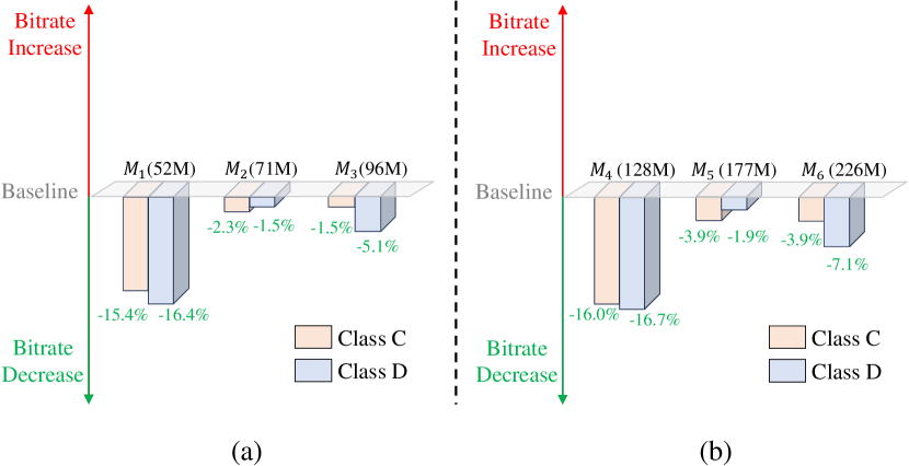
We increase the number of intermediate feature channels and insert more residual blocks to scale up the model size of the motion encoder and decoder. We build three models (, , ) with 52M, 71M, and 96M parameters, respectively. The comparison results as illustrated in Fig. 2(a) indicate that a slight increase in the model size of the motion encoder and decoder results in performance gains. However, continuously increasing the model size of the motion encoder-decoder will reduce the performance gain. For example, when the model size of the motion encoder-decoder is increased to 52M, 15.4% performance gain can be achieved for the HEVC Class C dataset. However, if we further increase its model size to 96M parameters, the performance gain drops to 1.5%. The results indicate that the motion encoder-decoder is not always the larger the better. More analysis can be found in Section V-C3. In addition, we observe that although larger motion encoder-decoders bring performance gain, the training processes become unstable and training crashes occur more frequently.
IV-A2 Scaling Up for Motion Entropy Model
Based on the abovementioned , , models, we first increase the channel number of the motion latent representation and associated hyperprior . Then, we scale up the model size of motion hyper-encoder, hyper-decoder, and quadtree partition-based spatial context models [32, 39] by increasing the number of intermediate feature channels. We build three models (, , ) with 128M, 177M, and 226M parameters, respectively. The comparison results as illustrated in Fig. 2(b) indicate that the increase in the model size of the motion entropy model can bring a little compression performance gain. For example, based on the model with 52M parameters, the model improves the performance gain from 15.4% to 16.0% for the HEVC Class C dataset. However, although , , models can further improve performance, similar to , , models, training crashes occur more frequently.
IV-A3 Scaling Up for Contextual Encoder-Decoder
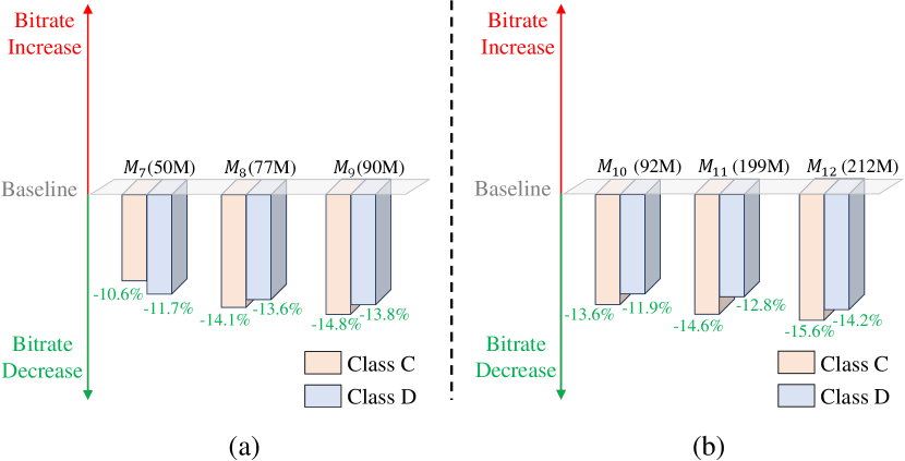
Based on our small baseline model with 21M parameters, we increase the number of intermediate feature channels and insert more residual blocks to scale up the model size of the contextual encoder and decoder. We build three models (, , ) with 50M, 77M, and 90M parameters, respectively. As presented in Fig. 3(a), increasing the model size of the context encoder and decoder can effectively improve compression performance. Different from the motion encoder and decoder, further increasing the model size of the contextual encoder and decoder can result in sustained and stable performance gains. For example, when the model size of the contextual encoder and decoder is increased to 50M, 10.6% performance gain can be achieved for the HEVC Class C dataset. When the model size of the contextual encoder and decoder is further increased to 90M, the performance gain can reach 14.8% for the HEVC Class C dataset. The results show that a larger contextual encoder-decoder can improve the transform capability. More analysis can be found in Section V-C1.
IV-A4 Scaling Up for Contextual Entropy Model
Based on , , models, we continue to scale up the model size of their contextual entropy models. We increase the channel number of the contextual latent representation and associated hyperprior . In addition, we increase the channel number of intermediate features of the contextual entropy model, including the contextual hyper-encoder, hyper-decoder, and quadtree partition-based spatial context models [32, 39]. We build three models (, , ) with 92M, 199M, and 212M parameters, respectively. As presented in Fig. 3(b), increasing the model size of the context encoder and decoder can bring stable compression performance improvement. For example, when the model size of model is increased from 90M to 212M by scaling up its contextual entropy model, an additional 0.8% performance gain can be achieved for the HEVC Class C dataset. The results show that a larger contextual entropy model can improve the entropy modeling of the contextual latent representation.
IV-A5 Scaling Up for Temporal Context Mining
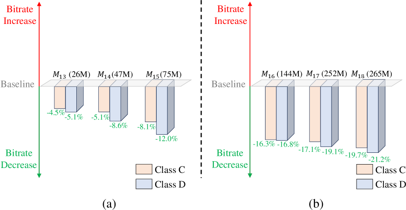
Temporal context mining is an intermediate link between the motion encoder-decoder and contextual encoder-decoder. To explore the influence of its model size, we increase the number of intermediate feature channels and insert more residual blocks to scale up its model size. Based on our small baseline model with 21M parameters, we build three models (, , ) with 26M, 47M, and 75M parameters, respectively. As shown in Fig. 4(a), scaling up the model size of the temporal context mining module can improve compression performance stably. For example, when the model size is increased from 26M to 75M, the performance gain can be increased from 5.1% to 12.0% for the HEVC Class D dataset. To explore whether the gain of scaling up the temporal context mining module can be superimposed with the gain of scaling up the contextual encoder-decoder and contextual entropy model, based on , , , we build another three models (, , ) with 144M, 252M, and 265M parameters, respectively. As shown in Fig. 4(b), based on the model with a larger contextual encoder-decoder and contextual entropy model, scaling up the model size of the temporal context mining module can bring additional performance gain. For example, based on with 212M parameters, increasing its temporal context mining module to build the model with 265M parameters can make the performance gain increase from 14.2% to 21.2% for the HEVC Class D dataset. The results show that a larger temporal context mining module can help make full use of the temporal correlation. More analysis can be found in Section V-C2.
IV-B Influence of Model Architecture
In addition to exploring the influence of model size, we also explore the influence of model architecture. In Section IV-A, all the models adopt CNN architectures. In this section, we try to replace the CNN architecture with mixed CNN-Transformer or Transformer architecture. Since the experimental results presented in Section IV-A indicate that scaling up the model sizes of contextual encoder-decoder, contextual entropy model, and temporal context mining module can bring stable compression performance improvement, we try new model architectures on these modules that have been proven to work.
IV-B1 Mixed CNN-Transformer Architecture
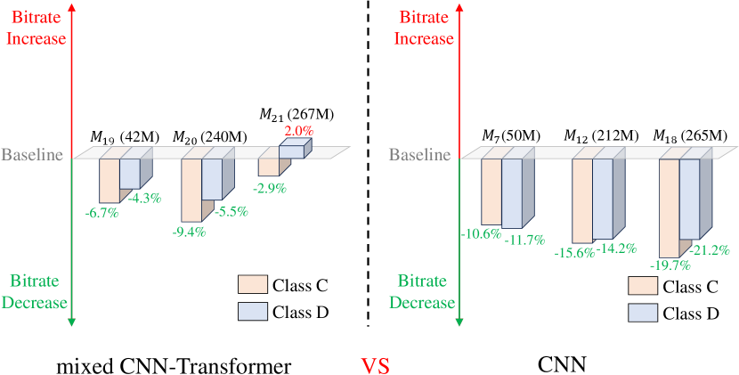
In terms of the mixed CNN-Transformer architecture, we build three models , , . For model , we replace the residual blocks between the convolutional layers of the contextual encoder and decoder with SwinTransformer layers [75] to build a contextual encoder-decoder with mixed CNN-Transformer architecture. We scale up its model size to 42M to compare it with its CNN-architecture counterpart— model (50M). For model , based on , we continue to insert SwinTransformer layers into the CNN-based entropy model to build a contextual entropy model with mixed CNN-Transformer architecture. We scale up its model size to 240M to compare it with its CNN architecture counterpart— model (212M). For model , based on , we insert a SwinTransformer layer after each residual block of the temporal context mining module. We scale up its model size to 267M to compare it with its CNN architecture counterpart— model (265M). As illustrated in Fig. 5(a), for model and model , inserting the Transformer layers into the original CNN architecture can bring performance gain over the small baseline model for its global feature extraction ability. This phenomenon is consistent with previous work [76, 77, 78] on image coding based on Transformer. However, when compared with their CNN-architecture counterparts of similar model sizes, CNN-architecture counterparts can obtain higher video coding performance gain. For example, comparing and , which both have larger contextual encoder-decoder and larger contextual entropy model, the performance gain of is 15.6% but that of is only 9.4% for the HEVC Class C dataset. For model , inserting SwinTransformer layers into the temporal context mining module brings performance loss. The compression performance gain drops from 9.4% achieved by to 2.9%. The results indicate that the global feature extraction ability of Transformer layers may not be suitable for learning multi-scale temporal contexts.
IV-B2 Transformer Architecture
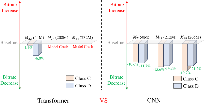
In terms of the Transformer architecture, we build three models , , . For model , we replace all the convolutional layers and residual blocks of the contextual encoder and decoder with SwinTransformer layers [75] to build a contextual encoder-decoder with Transformer architecture. We scale up its model size to 44M to compare it with its CNN-architecture counterpart— model (50M). For model , based on , we further replace the convolutional layers and depth blocks in the contextual entropy model with SwinTransformer layers to build a contextual entropy model with Transformer architecture. We scale up its model size to 208M to compare it with its CNN architecture counterpart— model (212M). For model , based on , we replace all the convolutional layers and residual blocks of the temporal context mining module with SwinTransformer layers. We scale up its model size to 232M to compare it with its CNN architecture counterpart— model (265M). As illustrated in Fig. 6, for model , the Transformer-based contextual encoder-decoder can bring a little performance gain over the small baseline model. However, when compared with its CNN architecture counterpart with similar model sizes, its performance gain is much smaller. For model and model , the Transform-only-based contextual entropy model and temporal context mining module make the model crash. Compared with the small baseline model, there is a PSNR loss of more than 4dB, which makes it difficult to calculate the BD-rate values. The results indicate that the convolutional layer is necessary for contextual entropy model and temporal context mining module.
| Number of Parameters | |
|---|---|
| Motion Estimation | 0.96M |
| Motion Encoder-Decoder | 0.81M |
| Motion Entropy Model | 2.50M |
| Contextual Encoder-Decoder | 504.59M |
| Contextual Entropy Model | 435.88M |
| Temporal Context Mining | 411.21M |
| Totally | 1355.95M (1.36B) |
IV-C Summary of Exploration Results
Based on the abovementioned exploration results, we make the following summary:
-
•
Slightly scaling up the model size of the motion encoder-decoder and motion entropy model brings compression performance gains, while further increasing the model size can lead to performance degradation.
-
•
Scaling up the model sizes of contextual encoder-decoder, contextual entropy model, and temporal context mining module can bring continuous compression performance improvement.
-
•
With a similar model size, the video coding model with CNN architecture can achieve higher compression performance than that with mixed CNN-Transformer and Transformer architectures.
According to the summary of exploration results, we build a large neural video coding model—NVC-1B with CNN architecture. Under the limited GPU memory condition, and in order to ensure the stability of training, we allocate most of the model parameters to the contextual encoder-decoder, contextual entropy model, and temporal context mining module. The number of parameters for each coding module of our proposed NVC-1B is listed in Table I.
IV-D Model Training
We design an elaborate training strategy for our proposed NVC-1B model, ensuring that each of its modules is fully trained. Table. II lists the detailed training stages. The training stages can be classified into 6 classes according to the training loss functions: , , , , , and . Among them, when using and as the loss functions, we only train the motion parts (Inter). When using and as the loss functions, we only train the temporal context mining and contextual parts (Rec). When using or as the loss function, we train all parts of the model (All).
| Frames | Network | Loss | Learning Rate | Epoch |
| 2 | Inter | 2 | ||
| 2 | Inter | 6 | ||
| 2 | Recon | 6 | ||
| 3 | Inter | 2 | ||
| 3 | Recon | 3 | ||
| 4 | Recon | 3 | ||
| 6 | Recon | 3 | ||
| 2 | Recon | 6 | ||
| 3 | Recon | 3 | ||
| 4 | Recon | 3 | ||
| 6 | Recon | 3 | ||
| 2 | All | 15 | ||
| 3 | All | 15 | ||
| 4 | All | 15 | ||
| 6 | All | 10 | ||
| 6 | All | 10 | ||
| 6 | All | 5 | ||
| 6 | All | 2 | ||
| 6 | All | 2 | ||
| 6 | All | 2 | ||
| 6 | All | 4 |
-
•
As described in (1), calculates the distortion between and its warping frame , which is used to obtain the high-fidelity reconstructed motion vectors.
(1) -
•
As described in (2), based on , takes the trade-off between the fidelity and the consumed bitrate of motion vectors into account. denotes the joint bitrate used for encoding the quantized motion latent representation and its associated hyperprior.
(2) -
•
As described in (3), calculates the distortion between and its reconstructed frame , which is used to generate a high-quality reconstructed frame.
(3) -
•
As described in (4), based on , takes the trade-off between the quality of reconstructed frame and the consumed bitrate of contextual latent representation . denotes the joint bitrate used for encoding the quantized contextual latent representation and its associated hyperprior.
(4) -
•
As described in (5), takes the trade-off between the quality of the reconstructed frame and all the consumed bitrate of the coded frame into account.
(5) - •
We use the Lagrangian multiplier to control the trade-off between the bitrate and distortion. To reduce the error propagation, we follow [32, 39] and add a periodically varying weight for each P-frame before the Lagrangian multiplier .
| HEVC Class B | HEVC Class C | HEVC Class D | HEVC Class E | UVG | MCL-JCV | Average | |
| VTM | 0.0 | 0.0 | 0.0 | 0.0 | 0.0 | 0.0 | 0.0 |
| HM | 39.0 | 37.6 | 34.7 | 48.6 | 36.4 | 41.9 | 39.7 |
| CANF-VC | 58.2 | 73.0 | 48.8 | 116.8 | 56.3 | 60.5 | 68.9 |
| DCVC | 115.7 | 150.8 | 106.4 | 257.5 | 129.5 | 103.9 | 144.0 |
| DCVC-TCM | 32.8 | 62.1 | 29.0 | 75.8 | 23.1 | 38.2 | 43.5 |
| DCVC-HEM | –0.7 | 16.1 | –7.1 | 20.9 | –17.2 | –1.6 | 1.73 |
| DCVC-DC | –13.9 | –8.8 | –27.7 | –19.1 | –25.9 | –14.4 | –18.3 |
| DCVC-FM | –8.8 | –5.0 | –23.3 | –20.8 | –20.5 | –7.4 | –14.3 |
| DCVC-SDD | –13.7 | –2.3 | –24.9 | –8.4 | –19.7 | –7.1 | –12.7 |
| Ours | –27.0 | –21.2 | –37.0 | –15.4 | –28.7 | –21.3 | –25.1 |
-
•
†DCVC-SDD [32] is our small baseline model.
| HEVC Class B | HEVC Class C | HEVC Class D | HEVC Class E | UVG | MCL-JCV | Average | |
| VTM | 0.0 | 0.0 | 0.0 | 0.0 | 0.0 | 0.0 | 0.0 |
| ECM | –19.5 | –21.5 | –20.1 | –18.8 | –15.5 | –18.3 | –19.0 |
| HM | 41.1 | 36.6 | 32.1 | 44.7 | 38.1 | 43.5 | 39.4 |
| DCVC-DC | –11.6 | –13.1 | –28.8 | –18.1 | –17.2 | –11.0 | –16.6 |
| DCVC-FM | –16.6 | –17.7 | –33.4 | –29.9 | –25.0 | –15.6 | –23.0 |
| DCVC-SDD | –4.2 | –2.3 | –25.7 | –10.6 | –7.0 | –0.3 | –8.4 |
| Ours | –17.7 | –21.8 | –37.4 | –14.0 | –16.0 | –15.9 | –20.5 |
| Schemes | Enc Time | Dec Time |
|---|---|---|
| VTM | 743.88 s | 0.31 s |
| ECM | 5793.88 s | 1.28 s |
| HM | 92.58 s | 0.21 s |
| DCVC-SDD | 0.89 s | 0.70 s |
| Ours | 4.44 s | 3.54 s |
V Experiments
V-A Experimental Setup
V-A1 Training and Testing Data
For training, we use 7-frame videos of the Vimeo-90k [80] dataset. Following most existing neural video coding models [34, 30, 35, 32], we randomly crop the original videos into 256256 patches for data augmentation. For testing, we use HEVC dataset [81], UVG dataset [82], and MCL-JCV dataset [83] in RGB and YUV420 format. These datasets contain videos with different contents, motion patterns, and resolutions, which are commonly used to evaluate the performance of neural video coding models. When testing RGB videos, we convert the videos in YUV420 format to RGB format using FFmpeg.
V-A2 Implementation Details
Following [32, 39], we set 4 base values (85, 170, 380, 840) to control the rate-distortion trade-off. For hierarchical quality, we set the periodically varying weight before as (0.5, 1.2, 0.5, 0.9). We implement our NVC-1B model with PyTorch. AdamW [84] is used as the optimizer and batch size is set to 32. Before the multi-frame cascaded fine-tuning stage, we train the NVC-1B model on 32 NVIDIA Ampere Tesla A40 (48G memory) GPUs for 85 days. In the multi-frame cascaded fine-tuning stage, we train the NVC-1B model on 4 NVIDIA A800 PCIe (80G memory) GPUs for 28 days. To alleviate the CUDA memory pressure induced by multi-frame cascaded training, Forward Recomputation Backpropagation (FRB)111https://qywu.github.io/2019/05/22/explore-gradient-checkpointing.html is used.
V-A3 Test Configurations
As with most previous neural video coding models, we focus on the low-delay coding scenario in this paper. Following [30, 32, 39, 34], we test 96 frames for each video sequence and set the intra-period to 32. For traditional video codecs, we choose HM-16.20 [85], VTM-13.2 [49], and ECM-5.0 [79] as our benchmarks. HM-16.20 is the official reference software of H.265/HEVC. VTM-13.2 is the official reference software of H.266/VVC. ECM is the prototype of the next-generation traditional codec. We use encoder_lowdelay_main (_rext), encoder_lowdelay_vtm, , and encoder_lowdelay_ecm configurations for HM-16.20, VTM-13.2, and ECM-13.0, respectively. The detailed commands for HM-16.20, VTM-13.2, and ECM-13.0 are shown as follows.
-
•
-c --InputFile= --InputChromaFormat= --FrameRate= --DecodingRefreshType=2 --InputBitDepth=8 --FramesToBeEncoded=96 --SourceWidth= --SourceHeight= --IntraPeriod=32 --QP= --Level=6.2 --BitstreamFile=
For neural video coding models, we choose CANF-VC [36], DCVC [34], DCVC-TCM [30], DCVC-HEM [35], DCVC-DC [35], DCVC-FM [40], and our small baseline model—DCVC-SDD [32] as our benchmarks.
V-A4 Evaluation Metrics
When testing RGB videos, we use RGB-PSNR as the distortion evaluation metric. When testing YUV420 videos, following DCVC-DC [35], we use the compound YUV PSNR as the distortion evaluation metric. The weight of YUV components is set to 6:1:1 [86]. Bits per pixel (bpp) is used as the bitrate evaluation metric. BD-rate [87] is used to compare the compression performance of difference models, where negative numbers indicate bitrate saving and positive numbers indicate bitrate increasing.
V-B Experimental Results
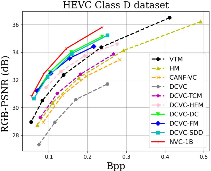
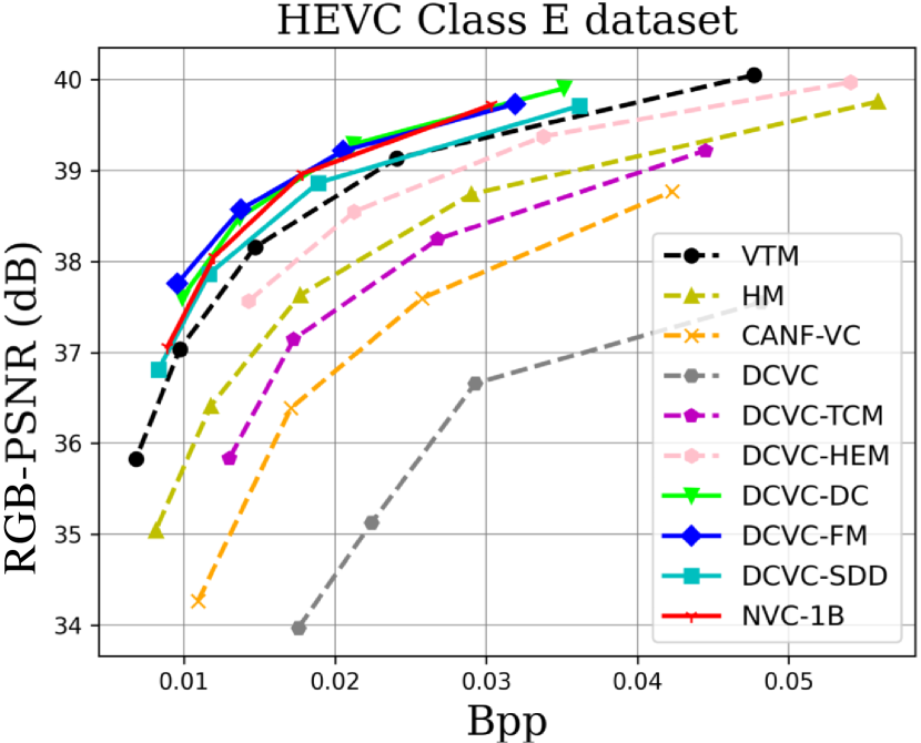
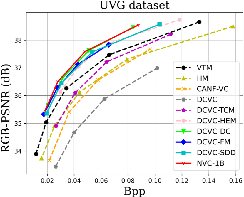
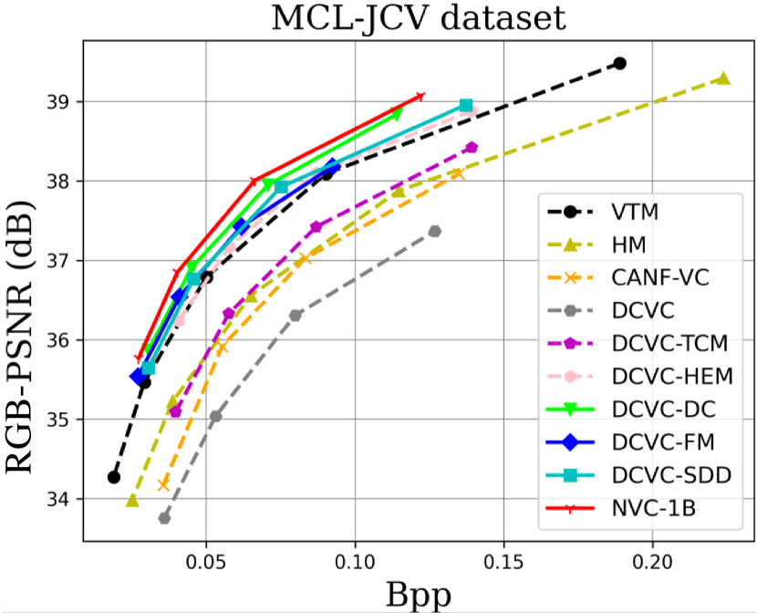
V-B1 Objective Comparison Results for RGB Videos
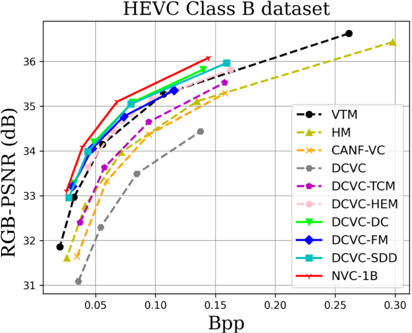
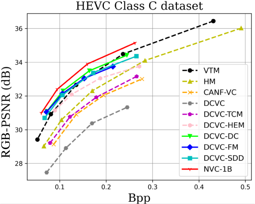
When testing RGB videos, we illustrate the rate-distortion curves on the HEVC, UVG, and MCL-JCV RGB video datasets in Fig. 7. The curves show that our proposed large neural video coding model—NVC-1B has significantly outperformed its small baseline model—DCVC-SDD. We list the detailed BD-rate comparison results in Table. III. The results show that our NVC-1B achieves an average –25.1% BD-rate reduction over VTM-13.2 across all test datasets, which is much better than that of DCVC-SDD (–12.7%). It even surpasses the state-of-the-art neural video coding models—DCVC-DC (–18.3%) and DCVC-FM (–14.3%).
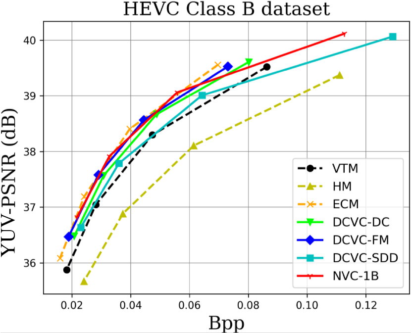
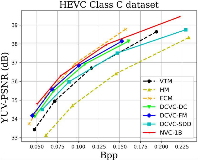
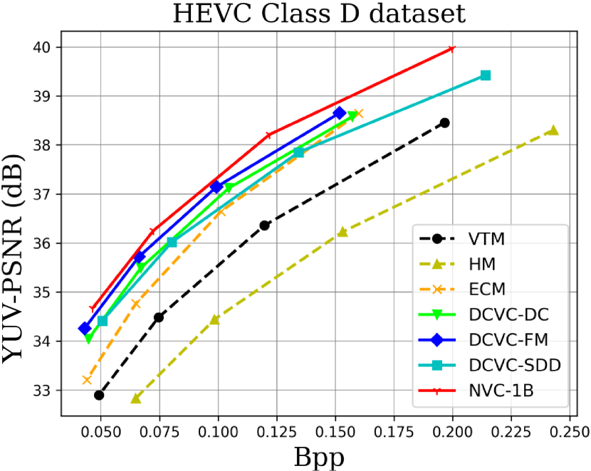
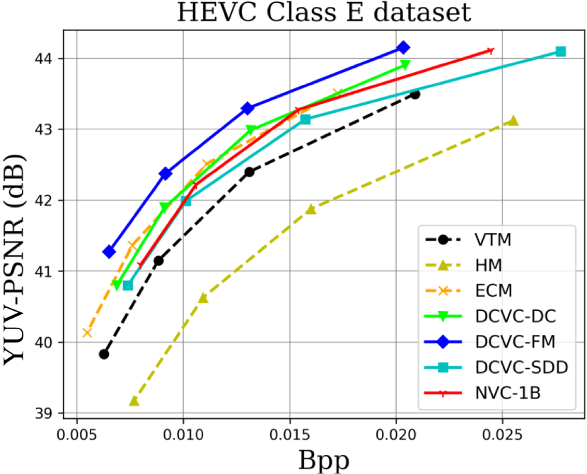
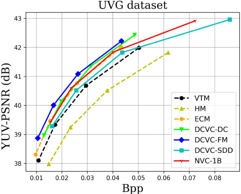
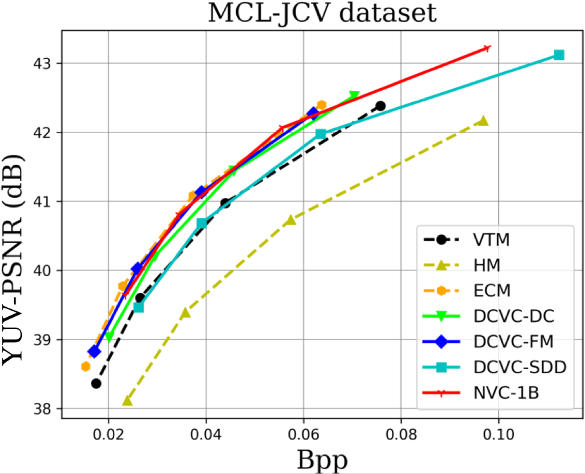
When testing YUV420 videos, we illustrate the rate-distortion curves on the YUV420 videos in Fig. 8 and list the corresponding BD-rate comparison results in Table. IV. The results show that based on our small baseline model—DCVC-SDD, the large model improves the average compression performance from –8.4% to –20.5%, which even outperforms ECM (–19.0%).
However, we find that the performance gain on the HEVC Class E dataset is smaller than that of other datasets. This is mainly because the number of frames used for multi-frame cascaded fine-tuning is small (6 frames) under the limitation of GPU CUDA memory. If we have GPUs with larger CUDA memory, we can use more frames (DCVC-DC uses 7 frames and DCVC-FM uses 32 frames) to fine-tune our large model to improve its compression performance.
V-B2 Subjective Comparison Results
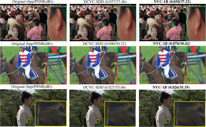
We visualize the reconstructed frames of our proposed NVC-1B and its small baseline model—DCVC-SDD in Fig. 9. By comparing their subjective qualities, we observe that the frames reconstructed by NVC-1B can retain more textures with a lower bitrate. We take the videoSRC14 sequence of the MCL-JCV dataset, the RaceHorses sequence of the HEVC Class D dataset, and the Kimono1 sequence of the HEVC Class B dataset as examples. For the videoSRC14 sequence, our NVC-1B model can use the bitrate of 0.051 bpp (0.057 bpp for DCVC-SDD) to achieve a reconstructed frame of 37.52 dB (37.46 dB for DCVC-SDD). Observing the earring of the dancing woman in videoSRC14, we can find our NVC-1B model can keep sharper edges. For the RaceHorses sequence, our NVC-1B model can use the bitrate of 0.078 bpp (0.090 bpp for DCVC-SDD) to achieve a reconstructed frame of 30.42 dB (30.32 dB for DCVC-SDD). Comparing the horse’s reins, we can see that our NVC-1B model can reconstruct the reins but DCVC-SDD cannot. For the Kimino1 sequence, our NVC-1B model can use the bitrate of 0.026 bpp (0.027 bpp for DCVC-SDD) to achieve a reconstructed frame of 35.19 dB (35.06 dB for DCVC-SDD). Zooming in the belt on the woman, the frame reconstructed by our NVC-1B model can retain more details.
V-B3 Encoding/Decoding Time
Following the setting of our small baseline model—DCVC-SDD, we include the time for model inference, entropy modeling, entropy coding, and data transfer between CPU and GPU. All the learned video codecs are run on a NVIDIA A800 GPU. As shown in Table V, the encoding and decoding time of our NVC-1B model for 1080p video are 4.44s and 3.54s per frame, respectively, which are five times longer than that of DCVC-SDD. However, the encoding time of our NVC-1B model is significantly lower than that of traditional video codecs. With the development of lightweight techniques [88, 89] for large models, the encoding and decoding time can be further optimized.
V-C Analysis
V-C1 Analysis of Transform Energy Compaction
To explore why our proposed large video coding model—NVC-1B can bring performance gain, we analyze the transform energy compaction. We calculate the average bitrate ratio of each channel of the contextual latent representation over the HEVC Class C and D datasets. Specifically, the contextual bitrate ratio (CR) of channel for each video sequence is first calculated as (7).
| (7) |
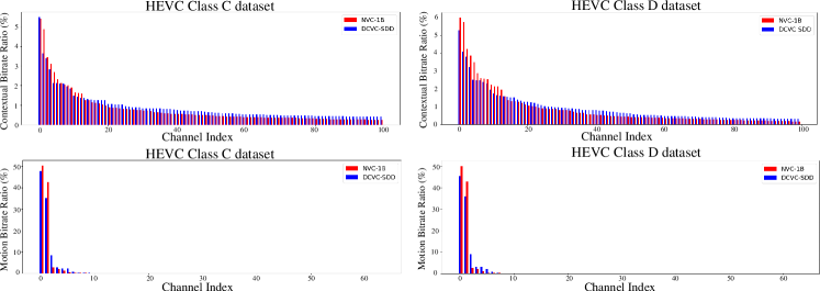
Then, we calculate the average contextual bitrate ratio over all sequences. We sort the average contextual bitrate ratio of each channel from largest to smallest to analyze the transform energy compaction. As illustrated in Fig. 10, for contextual bitrate ratio, we present the top 100 channels with obvious bitrate overhead. Comparing the channel bitrate distribution, we find that the contextual latent representations generated by our proposed large video coding model have higher transform energy compaction than our small baseline model—DCVC-SDD. More bitrates are concentrated in fewer channels.
In addition to the contextual latent representations, we also calculate the channel bitrate ratio of motion latent representations . Similarly, the motion bitrate ratio (MR) of channel for each video sequence is first calculated as (8).
| (8) |
Then, we calculate the average motion bitrate ratio over all sequences. As presented in Fig. 10, by ranking the average motion bitrate ratio of each channel, we find that although we allocate most of the parameters to contextual parts, the transform energy compaction can be improved for motion compression by end-to-end training. The motion channel bitrate distribution of our large model is also more concentrated. The analysis indicates that our large video coding model can obtain a higher compression performance by increasing the transform energy compaction. More signal energy is concentrated in fewer channels, which is beneficial for entropy coding.
V-C2 Analysis of Temporal Context Mining Accuracy
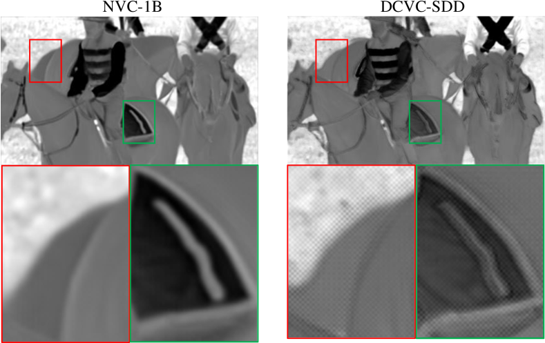
We further analyze the temporal context mining accuracy to explore why our proposed large video coding model—NVC-1B can bring performance gain. We visualize the temporal context predicted by NVC-1B and its small baseline model—DCVC-SDD in Fig. 11. By zooming in the temporal contexts, we find that the context predicted by NVC-1B has smoother object edges, whereas that predicted by DCVC-SDD has obvious prediction artifacts. For example, the edges of the horse’s tail and saddle predicted by DCVC-SDD have much noise, which seriously reduces the temporal prediction accuracy. The analysis indicates that our NVC-1B model can obtain a higher compression performance by improving the temporal context mining accuracy.
V-C3 Analysis of Scaling Up for Motion Encoder-Decoder
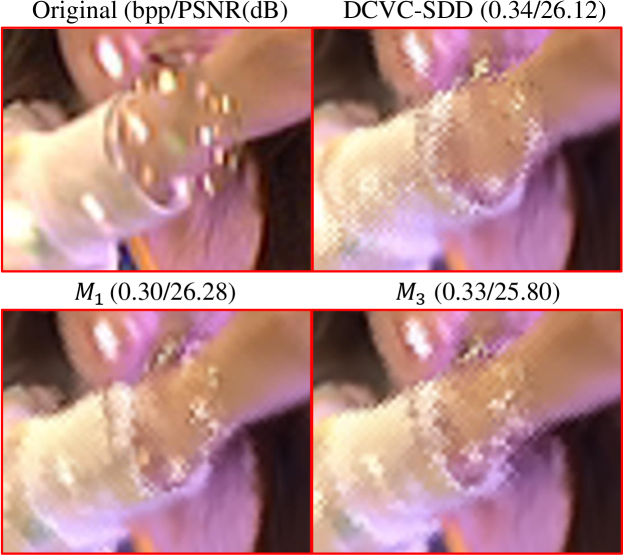
In Section IV-A1, we observe a strange phenomenon that if we slightly increase the model size of the motion encoder and decoder it can lead to performance gains. However, the performance gain will decrease if we continuously increase their model size. To explore the reason for this strange phenomenon, we visualize the warp frames predicted by the small baseline model—DCVC-SDD, , and models mentioned in Section IV-A1. As illustrated in Fig. 12, we find that, at a similar bitrate, the model with 52M parameters can obtain a more accurate warp frame than DCVC-SDD with 21M parameters. The arm and bubbles predicted by the model have fewer artifacts. However, the accuracy of the warp frame predicted by decreases dramatically. Its prediction artifacts of arms and bubbles increase significantly. The analysis indicates that the model size of the motion encoder-decoder is not always the bigger the better. An inappropriate model size will reduce the accuracy of temporal prediction.
VI Conclusion
In this paper, we scale up the model sizes of different parts of a neural video coding model to analyze the influence of model size on compression performance. In addition, we use different architectures to implement a neural video coding model to analyze the influence of model architecture architecture on compression performance. Based on our exploration, we design the first large neural video coding model—NVC-1B. Experimental results show that our proposed NVC-1B model can achieve a significant video compression gain over its small baseline model. In the future, we will design larger models with more efficient architectures to further improve the video compression performance.
References
- [1] T. Wiegand, G. J. Sullivan, G. Bjontegaard, and A. Luthra, “Overview of the H.264/AVC video coding standard,” IEEE Transactions on Circuits and Systems for Video Technology, vol. 13, no. 7, pp. 560–576, 2003.
- [2] G. J. Sullivan, J.-R. Ohm, W.-J. Han, and T. Wiegand, “Overview of the high efficiency video coding (HEVC) standard,” IEEE Transactions on Circuits and Systems for Video Technology, vol. 22, no. 12, pp. 1649–1668, 2012.
- [3] B. Bross, Y.-K. Wang, Y. Ye, S. Liu, J. Chen, G. J. Sullivan, and J.-R. Ohm, “Overview of the versatile video coding (VVC) standard and its applications,” IEEE Transactions on Circuits and Systems for Video Technology, 2021.
- [4] A. Habibian, T. v. Rozendaal, J. M. Tomczak, and T. S. Cohen, “Video compression with rate-distortion autoencoders,” in Proceedings of the IEEE/CVF International Conference on Computer Vision (ICCV), October 2019.
- [5] W. Sun, C. Tang, W. Li, Z. Yuan, H. Yang, and Y. Liu, “High-quality single-model deep video compression with frame-conv3d and multi-frame differential modulation,” in European Conference on Computer Vision (ECCV), pp. 239–254, Springer, 2020.
- [6] J. Liu, S. Wang, W.-C. Ma, M. Shah, R. Hu, P. Dhawan, and R. Urtasun, “Conditional entropy coding for efficient video compression,” in European Conference on Computer Vision (ECCV), pp. 453–468, Springer, 2020.
- [7] F. Mentzer, G. Toderici, D. Minnen, S. Caelles, S. J. Hwang, M. Lucic, and E. Agustsson, “VCT: A video compression transformer,” in Advances in Neural Information Processing Systems (NeurIPS), 2022.
- [8] H. Chen, B. He, H. Wang, Y. Ren, S. N. Lim, and A. Shrivastava, “Nerv: Neural representations for videos,” Advances in Neural Information Processing Systems, vol. 34, pp. 21557–21568, 2021.
- [9] H. Chen, M. Gwilliam, S.-N. Lim, and A. Shrivastava, “Hnerv: A hybrid neural representation for videos,” in Proceedings of the IEEE/CVF Conference on Computer Vision and Pattern Recognition, pp. 10270–10279, 2023.
- [10] Q. Zhao, M. S. Asif, and Z. Ma, “Dnerv: Modeling inherent dynamics via difference neural representation for videos,” in Proceedings of the IEEE/CVF Conference on Computer Vision and Pattern Recognition, pp. 2031–2040, 2023.
- [11] H. M. Kwan, G. Gao, F. Zhang, A. Gower, and D. Bull, “Hinerv: Video compression with hierarchical encoding-based neural representation,” Advances in Neural Information Processing Systems, vol. 36, 2024.
- [12] H. Liu, H. Shen, L. Huang, M. Lu, T. Chen, and Z. Ma, “Learned video compression via joint spatial-temporal correlation exploration,” in Proceedings of the AAAI Conference on Artificial Intelligence, vol. 34, pp. 11580–11587, 2020.
- [13] O. Rippel, A. G. Anderson, K. Tatwawadi, S. Nair, C. Lytle, and L. Bourdev, “ELF-VC: Efficient learned flexible-rate video coding,” in Proceedings of the IEEE/CVF International Conference on Computer Vision (ICCV), pp. 14479–14488, October 2021.
- [14] G. Lu, X. Zhang, W. Ouyang, L. Chen, Z. Gao, and D. Xu, “An end-to-end learning framework for video compression,” IEEE Transactions on Pattern Analysis and Machine Intelligence, 2020.
- [15] J. Lin, D. Liu, H. Li, and F. Wu, “M-LVC: multiple frames prediction for learned video compression,” in Proceedings of the IEEE/CVF Conference on Computer Vision and Pattern Recognition (CVPR), pp. 3546–3554, 2020.
- [16] Z. Hu, G. Lu, and D. Xu, “FVC: A new framework towards deep video compression in feature space,” in Proceedings of the IEEE/CVF Conference on Computer Vision and Pattern Recognition (CVPR), pp. 1502–1511, 2021.
- [17] E. Agustsson, D. Minnen, N. Johnston, J. Balle, S. J. Hwang, and G. Toderici, “Scale-space flow for end-to-end optimized video compression,” in Proceedings of the IEEE/CVF Conference on Computer Vision and Pattern Recognition (CVPR), pp. 8503–8512, 2020.
- [18] Z. Cheng, H. Sun, M. Takeuchi, and J. Katto, “Learning image and video compression through spatial-temporal energy compaction,” in Proceedings of the IEEE/CVF Conference on Computer Vision and Pattern Recognition (CVPR), pp. 10071–10080, 2019.
- [19] O. Rippel, S. Nair, C. Lew, S. Branson, A. G. Anderson, and L. Bourdev, “Learned video compression,” in Proceedings of the IEEE/CVF International Conference on Computer Vision (ICCV), pp. 3454–3463, 2019.
- [20] A. Djelouah, J. Campos, S. Schaub-Meyer, and C. Schroers, “Neural inter-frame compression for video coding,” in Proceedings of the IEEE/CVF International Conference on Computer Vision (ICCV), pp. 6421–6429, 2019.
- [21] R. Yang, F. Mentzer, L. Van Gool, and R. Timofte, “Learning for video compression with recurrent auto-encoder and recurrent probability model,” IEEE Journal of Selected Topics in Signal Processing, vol. 15, no. 2, pp. 388–401, 2021.
- [22] B. Liu, Y. Chen, S. Liu, and H.-S. Kim, “Deep learning in latent space for video prediction and compression,” in Proceedings of the IEEE/CVF Conference on Computer Vision and Pattern Recognition (CVPR), pp. 701–710, 2021.
- [23] H. Liu, M. Lu, Z. Ma, F. Wang, Z. Xie, X. Cao, and Y. Wang, “Neural video coding using multiscale motion compensation and spatiotemporal context model,” IEEE Transactions on Circuits and Systems for Video Technology, 2020.
- [24] M. A. Yılmaz and A. M. Tekalp, “End-to-end rate-distortion optimized learned hierarchical bi-directional video compression,” IEEE Transactions on Image Processing, vol. 31, pp. 974–983, 2021.
- [25] Z. Chen, T. He, X. Jin, and F. Wu, “Learning for video compression,” IEEE Transactions on Circuits and Systems for Video Technology, vol. 30, no. 2, pp. 566–576, 2019.
- [26] K. Lin, C. Jia, X. Zhang, S. Wang, S. Ma, and W. Gao, “DMVC: Decomposed motion modeling for learned video compression,” IEEE Transactions on Circuits and Systems for Video Technology, 2022.
- [27] Z. Guo, R. Feng, Z. Zhang, X. Jin, and Z. Chen, “Learning cross-scale weighted prediction for efficient neural video compression,” IEEE Transactions on Image Processing, 2023.
- [28] H. Guo, S. Kwong, C. Jia, and S. Wang, “Enhanced motion compensation for deep video compression,” IEEE Signal Processing Letters, 2023.
- [29] R. Yang, R. Timofte, and L. Van Gool, “Advancing learned video compression with in-loop frame prediction,” IEEE Transactions on Circuits and Systems for Video Technology, 2022.
- [30] X. Sheng, J. Li, B. Li, L. Li, D. Liu, and Y. Lu, “Temporal context mining for learned video compression,” IEEE Transactions on Multimedia, 2022.
- [31] F. Wang, H. Ruan, F. Xiong, J. Yang, L. Li, and R. Wang, “Butterfly: Multiple reference frames feature propagation mechanism for neural video compression,” in 2023 Data Compression Conference (DCC), pp. 198–207, IEEE, 2023.
- [32] X. Sheng, L. Li, D. Liu, and H. Li, “Spatial decomposition and temporal fusion based inter prediction for learned video compression,” IEEE Transactions on Circuits and Systems for Video Technology, 2024.
- [33] X. Sheng, L. Li, D. Liu, and H. Li, “Vnvc: A versatile neural video coding framework for efficient human-machine vision,” IEEE Transactions on Pattern Analysis and Machine Intelligence, 2024.
- [34] J. Li, B. Li, and Y. Lu, “Deep contextual video compression,” Advances in Neural Information Processing Systems (NeurIPS), vol. 34, pp. 18114–18125, 2021.
- [35] J. Li, B. Li, and Y. Lu, “Hybrid spatial-temporal entropy modelling for neural video compression,” in Proceedings of the 30th ACM International Conference on Multimedia, pp. 1503–1511, 2022.
- [36] Y.-H. Ho, C.-P. Chang, P.-Y. Chen, A. Gnutti, and W.-H. Peng, “Canf-vc: Conditional augmented normalizing flows for video compression,” in Computer Vision–ECCV 2022: 17th European Conference, Tel Aviv, Israel, October 23–27, 2022, Proceedings, Part XVI, pp. 207–223, Springer, 2022.
- [37] D. Jin, J. Lei, B. Peng, Z. Pan, L. Li, and N. Ling, “Learned video compression with efficient temporal context learning,” IEEE Transactions on Image Processing, 2023.
- [38] R. Lin, M. Wang, P. Zhang, S. Wang, and S. Kwong, “Multiple hypotheses based motion compensation for learned video compression,” Neurocomputing, p. 126396, 2023.
- [39] J. Li, B. Li, and Y. Lu, “Neural video compression with diverse contexts,” in Proceedings of the IEEE/CVF Conference on Computer Vision and Pattern Recognition (CVPR), pp. 22616–22626, 2023.
- [40] J. Li, B. Li, and Y. Lu, “Neural video compression with feature modulation,” arXiv preprint arXiv:2402.17414, 2024.
- [41] J. Kaplan, S. McCandlish, T. Henighan, T. B. Brown, B. Chess, R. Child, S. Gray, A. Radford, J. Wu, and D. Amodei, “Scaling laws for neural language models,” arXiv preprint arXiv:2001.08361, 2020.
- [42] T. Brown, B. Mann, N. Ryder, M. Subbiah, J. D. Kaplan, P. Dhariwal, A. Neelakantan, P. Shyam, G. Sastry, A. Askell, et al., “Language models are few-shot learners,” Advances in neural information processing systems, vol. 33, pp. 1877–1901, 2020.
- [43] J. Achiam, S. Adler, S. Agarwal, L. Ahmad, I. Akkaya, F. L. Aleman, D. Almeida, J. Altenschmidt, S. Altman, S. Anadkat, et al., “Gpt-4 technical report,” arXiv preprint arXiv:2303.08774, 2023.
- [44] A. Kirillov, E. Mintun, N. Ravi, H. Mao, C. Rolland, L. Gustafson, T. Xiao, S. Whitehead, A. C. Berg, W.-Y. Lo, et al., “Segment anything,” in Proceedings of the IEEE/CVF International Conference on Computer Vision, pp. 4015–4026, 2023.
- [45] L. Yang, B. Kang, Z. Huang, X. Xu, J. Feng, and H. Zhao, “Depth anything: Unleashing the power of large-scale unlabeled data,” arXiv preprint arXiv:2401.10891, 2024.
- [46] A. Dosovitskiy, L. Beyer, A. Kolesnikov, D. Weissenborn, X. Zhai, T. Unterthiner, M. Dehghani, M. Minderer, G. Heigold, S. Gelly, et al., “An image is worth 16x16 words: Transformers for image recognition at scale,” arXiv preprint arXiv:2010.11929, 2020.
- [47] M. Dehghani, J. Djolonga, B. Mustafa, P. Padlewski, J. Heek, J. Gilmer, A. P. Steiner, M. Caron, R. Geirhos, I. Alabdulmohsin, et al., “Scaling vision transformers to 22 billion parameters,” in International Conference on Machine Learning, pp. 7480–7512, PMLR, 2023.
- [48] Z. Liu, H. Hu, Y. Lin, Z. Yao, Z. Xie, Y. Wei, J. Ning, Y. Cao, Z. Zhang, L. Dong, et al., “Swin transformer v2: Scaling up capacity and resolution,” in Proceedings of the IEEE/CVF conference on computer vision and pattern recognition, pp. 12009–12019, 2022.
- [49] “VTM-13.2.” https://vcgit.hhi.fraunhofer.de/jvet/VVCSoftware_VTM/. Accessed: 2022-03-02.
- [50] N. Du, Y. Huang, A. M. Dai, S. Tong, D. Lepikhin, Y. Xu, M. Krikun, Y. Zhou, A. W. Yu, O. Firat, et al., “Glam: Efficient scaling of language models with mixture-of-experts,” in International Conference on Machine Learning, pp. 5547–5569, PMLR, 2022.
- [51] A. Chowdhery, S. Narang, J. Devlin, M. Bosma, G. Mishra, A. Roberts, P. Barham, H. W. Chung, C. Sutton, S. Gehrmann, et al., “Palm: Scaling language modeling with pathways,” Journal of Machine Learning Research, vol. 24, no. 240, pp. 1–113, 2023.
- [52] R. Anil, A. M. Dai, O. Firat, M. Johnson, D. Lepikhin, A. Passos, S. Shakeri, E. Taropa, P. Bailey, Z. Chen, et al., “Palm 2 technical report,” arXiv preprint arXiv:2305.10403, 2023.
- [53] G. Team, R. Anil, S. Borgeaud, Y. Wu, J.-B. Alayrac, J. Yu, R. Soricut, J. Schalkwyk, A. M. Dai, A. Hauth, et al., “Gemini: a family of highly capable multimodal models,” arXiv preprint arXiv:2312.11805, 2023.
- [54] H. Touvron, T. Lavril, G. Izacard, X. Martinet, M.-A. Lachaux, T. Lacroix, B. Rozière, N. Goyal, E. Hambro, F. Azhar, et al., “Llama: Open and efficient foundation language models,” arXiv preprint arXiv:2302.13971, 2023.
- [55] A. Meta, “Introducing meta llama 3: The most capable openly available llm to date,” Meta AI., 2024.
- [56] X. Chen, X. Wang, S. Changpinyo, A. Piergiovanni, P. Padlewski, D. Salz, S. Goodman, A. Grycner, B. Mustafa, L. Beyer, et al., “Pali: A jointly-scaled multilingual language-image model,” arXiv preprint arXiv:2209.06794, 2022.
- [57] M. Cherti, R. Beaumont, R. Wightman, M. Wortsman, G. Ilharco, C. Gordon, C. Schuhmann, L. Schmidt, and J. Jitsev, “Reproducible scaling laws for contrastive language-image learning,” in Proceedings of the IEEE/CVF Conference on Computer Vision and Pattern Recognition, pp. 2818–2829, 2023.
- [58] A. Radford, J. W. Kim, C. Hallacy, A. Ramesh, G. Goh, S. Agarwal, G. Sastry, A. Askell, P. Mishkin, J. Clark, et al., “Learning transferable visual models from natural language supervision,” in International conference on machine learning, pp. 8748–8763, PMLR, 2021.
- [59] C.-Y. Wu, N. Singhal, and P. Krahenbuhl, “Video compression through image interpolation,” in Proceedings of the European Conference on Computer Vision (ECCV), pp. 416–431, 2018.
- [60] G. Lu, W. Ouyang, D. Xu, X. Zhang, C. Cai, and Z. Gao, “DVC: an end-to-end deep video compression framework,” in IEEE Conference on Computer Vision and Pattern Recognition, CVPR 2019, Long Beach, CA, USA, June 16-20, 2019, pp. 11006–11015, Computer Vision Foundation / IEEE, 2019.
- [61] Z. Hu, G. Lu, J. Guo, S. Liu, W. Jiang, and D. Xu, “Coarse-to-fine deep video coding with hyperprior-guided mode prediction,” in Proceedings of the IEEE/CVF Conference on Computer Vision and Pattern Recognition, pp. 5921–5930, 2022.
- [62] H. Liu, M. Lu, Z. Chen, X. Cao, Z. Ma, and Y. Wang, “End-to-end neural video coding using a compound spatiotemporal representation,” IEEE Transactions on Circuits and Systems for Video Technology, vol. 32, no. 8, pp. 5650–5662, 2022.
- [63] Y. Shi, Y. Ge, J. Wang, and J. Mao, “Alphavc: High-performance and efficient learned video compression,” in European Conference on Computer Vision, pp. 616–631, Springer, 2022.
- [64] J. Xiang, K. Tian, and J. Zhang, “Mimt: Masked image modeling transformer for video compression,” in The Eleventh International Conference on Learning Representations, 2022.
- [65] T. Xu, H. Gao, C. Gao, Y. Wang, D. He, J. Pi, J. Luo, Z. Zhu, M. Ye, H. Qin, et al., “Bit allocation using optimization,” in International Conference on Machine Learning, pp. 38377–38399, PMLR, 2023.
- [66] H. Kim, M. Bauer, L. Theis, J. R. Schwarz, and E. Dupont, “C3: High-performance and low-complexity neural compression from a single image or video,” arXiv preprint arXiv:2312.02753, 2023.
- [67] C. Tang, X. Sheng, Z. Li, H. Zhang, L. Li, and D. Liu, “Offline and online optical flow enhancement for deep video compression,” in Proceedings of the AAAI Conference on Artificial Intelligence, vol. 38, pp. 5118–5126, 2024.
- [68] M. Lu, Z. Duan, F. Zhu, and Z. Ma, “Deep hierarchical video compression,” in Proceedings of the AAAI Conference on Artificial Intelligence, vol. 38, pp. 8859–8867, 2024.
- [69] P. Du, Y. Liu, and N. Ling, “Cgvc-t: Contextual generative video compression with transformers,” IEEE Journal on Emerging and Selected Topics in Circuits and Systems, 2024.
- [70] J. Dai, H. Qi, Y. Xiong, Y. Li, G. Zhang, H. Hu, and Y. Wei, “Deformable convolutional networks,” in Proceedings of the IEEE international conference on computer vision, pp. 764–773, 2017.
- [71] B. Bross, J. Chen, J.-R. Ohm, G. J. Sullivan, and Y.-K. Wang, “Developments in international video coding standardization after avc, with an overview of versatile video coding (VVC),” Proceedings of the IEEE, 2021.
- [72] A. Ranjan and M. J. Black, “Optical flow estimation using a spatial pyramid network,” in Proceedings of the IEEE/CVF Conference on Computer Vision and Pattern Recognition (CVPR), pp. 4161–4170, 2017.
- [73] J. Ballé, V. Laparra, and E. P. Simoncelli, “End-to-end optimized image compression,” in International Conference on Learning Representations, (ICLR) 2017, Toulon, France, April 24-26, 2017, Conference Track Proceedings, 2017.
- [74] J. Ballé, D. Minnen, S. Singh, S. J. Hwang, and N. Johnston, “Variational image compression with a scale hyperprior,” in 6th International Conference on Learning Representations, ICLR 2018, Vancouver, BC, Canada, April 30 - May 3, 2018, Conference Track Proceedings, OpenReview.net, 2018.
- [75] Z. Liu, Y. Lin, Y. Cao, H. Hu, Y. Wei, Z. Zhang, S. Lin, and B. Guo, “Swin transformer: Hierarchical vision transformer using shifted windows,” in Proceedings of the IEEE/CVF International Conference on Computer Vision (ICCV), 2021.
- [76] M. Lu, P. Guo, H. Shi, C. Cao, and Z. Ma, “Transformer-based image compression,” arXiv preprint arXiv:2111.06707, 2021.
- [77] Y. Qian, M. Lin, X. Sun, Z. Tan, and R. Jin, “Entroformer: A transformer-based entropy model for learned image compression,” arXiv preprint arXiv:2202.05492, 2022.
- [78] J. Liu, H. Sun, and J. Katto, “Learned image compression with mixed transformer-cnn architectures,” in Proceedings of the IEEE/CVF conference on computer vision and pattern recognition, pp. 14388–14397, 2023.
- [79] “ECM-13.0.” https://vcgit.hhi.fraunhofer.de/ecm/ECM. Accessed: 2024-07-20.
- [80] T. Xue, B. Chen, J. Wu, D. Wei, and W. T. Freeman, “Video enhancement with task-oriented flow,” International Journal of Computer Vision, vol. 127, no. 8, pp. 1106–1125, 2019.
- [81] F. Bossen, “Common hm test conditions and software reference configurations (JCTVC-l1100),” Joint Collaborative Team on Video Coding (JCT-VC) of ITU-T SG, 2013.
- [82] A. Mercat, M. Viitanen, and J. Vanne, “UVG dataset: 50/120fps 4k sequences for video codec analysis and development,” in Proceedings of the 11th ACM Multimedia Systems Conference, pp. 297–302, 2020.
- [83] H. Wang, W. Gan, S. Hu, J. Y. Lin, L. Jin, L. Song, P. Wang, I. Katsavounidis, A. Aaron, and C.-C. J. Kuo, “MCL-JCV: a JND-based H.264/AVC video quality assessment dataset,” in 2016 IEEE International Conference on Image Processing (ICIP), pp. 1509–1513, IEEE, 2016.
- [84] D. P. Kingma and J. Ba, “Adam: A method for stochastic optimization,” arXiv preprint arXiv:1412.6980, 2014.
- [85] “HM-16.20.” https://vcgit.hhi.fraunhofer.de/jvet/HM/. Accessed: 2022-07-05.
- [86] J.-R. Ohm, G. J. Sullivan, H. Schwarz, T. K. Tan, and T. Wiegand, “Comparison of the coding efficiency of video coding standards—including high efficiency video coding (hevc),” IEEE Transactions on circuits and systems for video technology, vol. 22, no. 12, pp. 1669–1684, 2012.
- [87] G. Bjontegaard, “Calculation of average psnr differences between rd-curves,” VCEG-M33, 2001.
- [88] E. J. Hu, Y. Shen, P. Wallis, Z. Allen-Zhu, Y. Li, S. Wang, and W. Chen, “Lora: Low-rank adaptation of large language models,” arXiv preprint arXiv:2106.09685, 2021.
- [89] X. Lu, T. Xu, L. Zheng, Z. Wang, Y. S. Tian, I. Stoica, and J. E. Gonzalez, “Flexgen: High-throughput generative inference of large language models with a single gpu,” arXiv preprint arXiv:2303.06865, 2023.