This paper was converted on www.awesomepapers.org from LaTeX by an anonymous user.
Want to know more? Visit the Converter page.

Observability and State Estimation for a Class of Nonlinear Systems

John Tsinias and Constantinos Kitsos J. Tsinias is with the Department of Mathematics, National Technical University of Athens, Zografou Campus 15780, Athens, Greece, email:jtsin@central.ntua.gr (corresponding author). C. Kitsos is with the Department of Mathematics, National Technical University of Athens, Zografou Campus 15780, Athens, Greece and Univ. Grenoble Alpes, CNRS, Grenoble INP, GIPSA-lab, 38000 Grenoble, France, email: konstantinos.kitsos@gipsa-lab.grenoble-inp.fr\circ Institute of Engineering Univ. Grenoble Alpes
Abstract

We derive sufficient conditions for the solvability of the state estimation problem for a class of nonlinear control time-varying systems which includes those, whose dynamics have triangular structure. The state estimation is exhibited by means of a sequence of functionals approximating the unknown state of the system on a given bounded time interval. More assumptions guarantee solvability of the state estimation problem by means of a hybrid observer.

Index Terms:
nonlinear systems, observability, state estimation, hybrid observers.

I Introduction

Many important approaches have been presented in the literature concerning the state estimation problem for a given nonlinear control system (see for instance [1] - [19], [21] - [25], [27], [28] and relative references therein). Most of them are based on the existence of an observer system exhibiting state estimation. The corresponding hypotheses include observability assumptions and persistence of excitation. In [8], [9] and [10] Luenberger type observers and switching estimators are proposed for a general class of triangular systems under weaker assumptions than those adopted in the existing literature. In [16] and [24] the state estimation is exhibited for a class of systems by means of a hybrid observer.

The present note is inspired by the approach adopted in [16], where a ”hybrid dead-beat observer” is used, as well as by the methodologies applied in [20], [26] and [29], where, fixed point theorems are used for the establishment of sufficient conditions for observability and asymptotic controllability. Our main purpose is to establish that, under certain hypotheses, including persistence of excitation, the State Estimation Design Problem (SEDP) around a given fixed value of initial time is solvable for a class of nonlinear systems by means of a sequence of mappings XνX_{\nu}, exclusively dependent on the dynamics of the original system, the input uu and the corresponding output yy, and further each XνX_{\nu} is independent of the time-derivatives of uu and yy. An algorithm for explicit construction of these mappings is provided.

We consider time-varying finite dimensional nonlinear control systems of the form:

x˙=A(t,y,u)x+f(t,y,x,u)(t,y,x,u)0×k×n×m\displaystyle\begin{aligned} \dot{x}=A(t,y,u)x+f(t,y,x,u)\\ (t,y,x,u)\in{{\mathbb{R}}_{\geq 0}}\times{{\mathbb{R}}^{k}}\times{{\mathbb{R}}^{n}}\times{{\mathbb{R}}^{m}}\end{aligned} (1.1a)
with output
y=C(t,u)x\displaystyle y=C\left(t,u\right)x (1.1b)

where uu is the input of (1.1). Our main results establish sufficient conditions for the approximate solvability of the SEDP for (1.1). The paper is organized as follows. Section II contains definitions, assumptions, as well as statement and proof of our main result (Proposition 2.1) concerning the state estimation problem for the general case (1.1). We apply in Section III the main result of Section II for the derivation of sufficient conditions for the solvability of the same problem for certain subclasses of systems (1.1), whose dynamics have triangular structure (Proposition 3.1). According to our knowledge, the sufficient conditions proposed in Sections II, III are weaker than those imposed in the existing literature for the solvability of the observer design problem for the same class of systems. More extensions are discussed in Section IV of present work, concerning the solvability of the SEDP by means of a hybrid observer under certain additional assumptions (Proposition 4.1).

Notations: For given xnx\in{{\mathbb{R}}^{n}}, |x| \left|x\right|\text{ }denotes its usual Euclidean norm. For a given constant matrix Am×nA\in{{\mathbb{R}}^{m\times n}}, A{A}^{\prime} denotes its transpose and |A|:=sup{|Ax|,|x|=1}\left|A\right|:=\sup\left\{\left|Ax\right|,\left|x\right|=1\right\} is its induced norm. For any nonempty set II\subset\mathbb{R} and map ItA(t)m×nI\ni t\to A(t)\in{{\mathbb{R}}^{m\times n}} we adopt the notation A()I:=ess.sup{|A(t)|,tI}\|A(\cdot){{\|}_{I}}\text{:=}\operatorname{ess}.\sup\{\left|A(t)\right|,t\in I\}.

II Hypotheses and Main Result

In this section we provide sufficient conditions for observability of (1.1) and solvability of the SEDP. We assume that for each t0t\geq 0 the mappings A(t,,):A\left(t,\cdot,\cdot\right): k×mn×n{{\mathbb{R}}^{k}}\times{{\mathbb{R}}^{m}}\to{{\mathbb{R}}^{n\times n}} , C(t,):mk×nC\left(t,\cdot\right):{{\mathbb{R}}^{m}}\to{{\mathbb{R}}^{k\times n}} and f(t,,,):f\left(t,\cdot,\cdot,\cdot\right): k×n×mn{{\mathbb{R}}^{k}}\times{{\mathbb{R}}^{n}}\times{{\mathbb{R}}^{m}}\to{{\mathbb{R}}^{n}} are continuous and further ff is (locally) Lipschitz continuous with respect to xx, i.e., for every bounded I0,Xn,UmI\subset{{\mathbb{R}}_{\geq 0}},X\subset{{\mathbb{R}}^{n}},U\subset{{\mathbb{R}}^{m}} and YkY\subset{{\mathbb{R}}^{k}} there exists a constant C>0C>0 such that

|f(t,y,z1,u)f(t,y,z2,u)|C|z1z2|,\displaystyle\left|f\left(t,y,{{z}_{1}},u\right)-f\left(t,y,{{z}_{2}},u\right)\right|\leq C\left|{{z}_{1}}-{{z}_{2}}\right|,
(t,y,u)I×Y×U,z1,z2X\displaystyle\forall\left(t,y,u\right)\in I\times Y\times U,\,{{z}_{1}},{{z}_{2}}\in X (2.1)

Also, assume that for any (x,y,u)n×k×m\left(x,y,u\right)\in{{\mathbb{R}}^{n}}\times{{\mathbb{R}}^{k}}\times{{\mathbb{R}}^{m}} the mappings A(,y,u)A\left(\cdot,y,u\right), f(,y,x,u)f\left(\cdot,y,x,u\right) and C(,u)C(\cdot,u) are measurable and locally essentially bounded in 0\mathbb{R}_{\geq 0}. Let t00,τ>t0{{t}_{0}}\geq 0,\tau>{{t}_{0}} and let U[t0,τ]{{U}_{[{{t}_{0}},\tau]}} be a nonempty set of inputs uL([t0,τ];m)u\in{{L}_{\infty}}\left(\left[{{t}_{0}},\tau\right];{{\mathbb{R}}^{m}}\right) of (1.1) (without any loss of generality it is assumed that U[t0,τ]{{U}_{[{{t}_{0}},\tau]}} is independent of the initial state). Define by Y[t0,τ],u{{Y}_{[{{t}_{0}},\tau],u}} the set of outputs yy of (1.1) defined on the interval [t0,τ][{{t}_{0}},\tau] corresponding to some input uU[t0,τ]u\in{{U}_{[{{t}_{0}},\tau]}}:

Y[t0,τ],u:={yL([t0,τ];k):y(t)=C(t,u(t))\displaystyle Y_{[t_{0},\tau],u}:=\{y\in L_{\infty}\left([t_{0},\tau];\mathbb{R}^{k}\right):y(t)=C\left(t,u(t)\right)
×x(t;t0,x0,u),a.e. t[t0,τ], for certain x0n}\displaystyle\times x\left(t;t_{0},x_{0},u\right),\text{a.e. }t\in[t_{0},\tau],\text{ for certain }x_{0}\in\mathbb{R}^{n}\} (2.2)

provided that tmaxτ{{t}_{\max}}\geq\tau where tmax=tmax(t0,x0,u)+t_{\max}=t_{\max}(t_{0},x_{0},u)\leq+\infty is the maximum time of existence of the solution x(;t0,x0,u)x(\cdot;{{t}_{0}},{{x}_{0}},u) of (1.1) with initial x(t0;t0,x0,u)=x0x({{t}_{0}};{{t}_{0}},{{x}_{0}},u)={{x}_{0}}.

Definition II.1

Let II be a nonempty subset of 0{{\mathbb{R}}_{\geq 0}}. We say that (1.1) is observable over II, if for all t0I{{t}_{0}}\in I, almost all τ>t0\tau>{{t}_{0}} near t0{{t}_{0}}, input uU[t0,τ]u\in{{U}_{[{{t}_{0}},\tau]}} and output yY[t0,τ],uy\in{{Y}_{[{{t}_{0}},\tau],u}}, there exists a unique x0n{{x}_{0}}\in{{\mathbb{R}}^{n}} such that

y(t)=C(t,u(t))x(t;t0,x0,u),a.e. t[t0,τ]\displaystyle y(t)=C(t,u(t))x(t;{{t}_{0}},{{x}_{0}},u),\text{a.e. }t\in\left[{{t}_{0}},\tau\right] (2.3)

According to Definition 2.1, observability is equivalent to the existence of a (probably noncausal) functional X(,,):{t0}×Y[t0,τ],u×U[t0,τ]nX(\cdot,\cdot,\cdot):\left\{{{t}_{0}}\right\}\times{{Y}_{[{{t}_{0}},\tau],u}}\times{{U}_{[{{t}_{0}},\tau]}}\to{{\mathbb{R}}^{n}}, such that, for every x0n{{x}_{0}}\in{{\mathbb{R}}^{n}} for which (2.3) holds for certain uU[t0,τ]u\in{{U}_{[{{t}_{0}},\tau]}} and yY[t0,τ],uy\in{{Y}_{[{{t}_{0}},\tau],u}}, we have:

X(t0,y,u)=x0\displaystyle X({{t}_{0}},y,u)={{x}_{0}} (2.4)

and XX is exclusively dependent on the input uu and the output yy of (1.1) and is in general noncausal. Knowledge of XX satisfying the previous properties guarantees knowledge of the initial state value, thus knowledge of the future values of the solution of (1.1), provided that the system is complete.

Definition II.2

Let II be a nonempty subset of 0{{\mathbb{R}}_{\geq 0}}. We say that the SEDP is solvable for (1.1) over II, if there exists a functional X(,,):{t0}×Y[t0,τ],u×U[t0,τ]nX(\cdot,\cdot,\cdot):\left\{{{t}_{0}}\right\}\times{{Y}_{[{{t}_{0}},\tau],u}}\times{{U}_{[{{t}_{0}},\tau]}}\to{{\mathbb{R}}^{n}}, t0I{{t}_{0}}\in I, τ>t0\tau>{{t}_{0}} near t0{{t}_{0}}, being in general noncausal, such that (2.4) is fulfilled for every x0n{{x}_{0}}\in{{\mathbb{R}}^{n}} for which (2.3) holds for certain uU[t0,τ]u\in{{U}_{[{{t}_{0}},\tau]}} and further XX is exclusively depended on uu and yy and the dynamics of (1.1) and it does not include any differentiation of their arguments. It turns out that XX is independent of the time-derivatives of uu and yy, whenever they exist.

It is worthwhile to remark here that the approach proposed in [16] for the construction of a hybrid dead-beat observer for a subclass of systems (1.1) is based on an explicit construction of a (noncausal) map XX satisfying (2.4). However, for general nonlinear systems, the precise and direct determination of the functional XX is a difficult task. The difficulty comes from our requirements for the candidate XX to be exclusively dependent on uu and yy and the dynamics of system and, for practical reasons, it should be independent of the time-derivatives of uu and yy. We next provide a weaker sequential type of definition of the solvability of SEDP, which is adopted in the present work, in order to achieve the state determination for general case (1.1) by employing an explicit approximate strategy.

Definition II.3

We say that the approximate SEDP is solvable for system (1.1) over II, if there exist functionals Xν(,,),ν=1,2,:{t0}×Y[t0,τ],u×U[t0,τ]nX_{\nu}(\cdot,\cdot,\cdot),\nu=1,2,\ldots:\left\{{{t}_{0}}\right\}\times{{Y}_{[{{t}_{0}},\tau],u}}\times{{U}_{[{{t}_{0}},\tau]}}\to{{\mathbb{R}}^{n}}(being in general noncausal), such that, if we denote:

ξν:=Xν(t0,y,u),t0I,yY[t0,τ],u,uU[t0,τ]\displaystyle{{\xi}_{\nu}}:={{X}_{\nu}}({{t}_{0}},y,u),\ {{t}_{0}}\in I,y\in{{Y}_{[{{t}_{0}},\tau],u}},u\in{{U}_{[{{t}_{0}},\tau]}} (2.5)

then
(I) the mappings XνX_{\nu} are exclusively dependent on the input uu and the corresponding output yy, the dynamics of system (1.1) and further their domains do not include any differentiation of their arguments. It turns out that each XνX_{\nu} should be independent of the time-derivatives of uu and yy (whenever they exist);
(II) the following hold:

limνξν=x0;\displaystyle\lim_{\nu\to\infty}{{\xi}_{\nu}}={{x}_{0}}; (2.6a)
x0 is the (unique) vector forwhich both (2.3) and (2.6a) hold\displaystyle\begin{aligned} {{x}_{0}}\text{ is the (unique) vector for}\\ \text{which both (2.3) and (2.6a) hold}\end{aligned} (2.6b)

It should be emphasised that uniqueness requirement in (2.6b) is not essential. We may replace (2.6b) by the assumption that there exists x0x_{0} satisfying both (2.3) and (2.6a). Then uniqueness of such a vector x0x_{0} is a consequence of (2.6a), definition (2.5) and the fact that each functional XνX_{\nu} exclusively depends on uu and yy.

Obviously, according to the definitions above, the following implications hold:

Solvability of SEDP \Rightarrow Solvability of approximate SEDP \Rightarrow Observability (over II).
For completeness, we note that the first implication follows by setting Xν:=X,ν=1,2,X_{\nu}:=X,\nu=1,2,\ldots in (2.4). The second implication is a direct consequence of both assumptions (2.6a,b), definition (2.5) and the exclusive dependence of each XνX_{\nu} from uu and yy. The converse claims are not in general valid; particularly, observability does not in general imply solvability of the (approximate) SEDP, due to the additional requirements of Definitions 2.2 and 2.3 concerning the independence XX, XνX_{\nu}, respectively, from the time-derivatives of uu and yy.

From (2.6a) we deduce that, if the approximate SEDP is solvable for (1.1) over II, then for any T>t0T>t_{0} for which Ttmax(t0,x0,u)T\leq{{t}_{\max}}({{t}_{0}},{{x}_{0}},u) it holds:

limνx(;t0,ξν,u)x(;t0,x(t0),u)[t0,T]=0\displaystyle\lim_{\nu\to\infty}\|x(\cdot;t_{0},\xi_{\nu},u)-x(\cdot;t_{0},x(t_{0}),u)\|_{[t_{0},T]}=0 (2.7)
Remark II.1

(i) Condition (2.7) guarantees that for any given interval [t0,T][{{t}_{0}},T] with Ttmax(t0,x0,u)T\leq{{t}_{\max}}({{t}_{0}},{{x}_{0}},u), the unknown solution x(s;t0,x(t0),u),s[t0,T]x(s;{{t}_{0}},x({{t}_{0}}),u),s\in[{{t}_{0}},T] of (1.1) is uniformly approximated by a sequence of trajectories x^\hat{x} of the system

x^˙(t)=A(t,y,u)x^+f(t,y,x^,u),x^(to)=ξν,ν=1,2,\displaystyle\dot{\hat{x}}\left(t\right)=A(t,y,u)\hat{x}+f(t,y,\hat{x},u),\hat{x}({{t}_{o}})={{\xi}_{\nu}},\nu=1,2,\ldots

with ξν,ν=1,2,{{\xi}_{\nu}},\nu=1,2,\ldots as given in Definition 2.2.
(ii) If the system (1.1) is complete, then (2.7) implies solvability of the approximate SEDP, thus, observability for (1.1) over 0{{\mathbb{R}}_{\geq 0}}. Indeed, let t0I{{t}_{0}}\in I and without loss of generality consider arbitrary s>t0s>{{t}_{0}}. It follows by invoking the forward completeness assumption and (2.7) that limνξ^ν=x(s)\lim_{\nu\to\infty}{{\hat{\xi}}_{\nu}}=x(s), where ξ^ν:=x(s;t0,ξν,u),ν=1,2,{{\hat{\xi}}_{\nu}}:=x(s;{{t}_{0}},{{\xi}_{\nu}},u),\nu=1,2,\ldots and simultaneously (2.3) and (2.6a) hold with ss and x(s)x(s), instead of t0{{t}_{0}} and x0=x(t0){{x}_{0}}=x({{t}_{0}}), respectively. Moreover, due to the backward completeness, x(s)x(s) is the unique vector for which limνξ^ν=x(s)\lim_{\nu\to\infty}{{\hat{\xi}}_{\nu}}=x(s).

In order to state and establish our main result, we first require the following notations and additional assumptions for the dynamics of (1.1). Consider t0I{{t}_{0}}\in I, τ>t0\tau>{{t}_{0}}, uU[t0,τ]u\in{{U}_{[{{t}_{0}},\tau]}}, yY[t0,τ],uy\in{{Y}_{[{{t}_{0}},\tau],u}} and dC0([t0,τ];m)d\in{{C}^{0}}\left(\left[{{t}_{0}},\tau\right];{{\mathbb{R}}^{m}}\right). We denote by Φ(t,t0)\Phi(t,{{t}_{0}}) the fundamental matrix solution of

tΦ(t,t0)=A(t,y(t),u(t))Φ(t,t0)\displaystyle\frac{\partial}{\partial t}\Phi(t,{{t}_{0}})=A(t,y(t),u(t))\Phi(t,{{t}_{0}}) (2.8a)
Φ(t0,t0)=In×n\displaystyle\Phi\left({{t}_{0}},{{t}_{0}}\right)={{I}_{n\times n}} (2.8b)

and define the mappings:

Ψ(t;t0,y,u):=t0tΦ(s,t0)C(s,u(s))C(s,u(s))Φ(s,t0)𝑑s,t[t0,τ]\Psi\left(t;{{t}_{0}},y,u\right):=\\ \int\limits_{{{t}_{0}}}^{t}{\Phi^{\prime}\left(s,{{t}_{0}}\right)C^{\prime}\left(s,u\left(s\right)\right)C\left(s,u\left(s\right)\right)\Phi\left(s,{{t}_{0}}\right)ds},t\in\left[{{t}_{0}},\tau\right] (2.9)
Ξ(t;t0,y,d,u):=t0tΦ(ρ,t0)C(ρ,u(ρ))C(ρ,u(ρ))Φ(ρ,t0)×(t0ρΦ(t0,s)f(s,y(s),d(s),u(s))ds)dρ,t[t0,τ]{{\Xi}}(t;{{t}_{0}},y,d,u):=\int_{{{t}_{0}}}^{t}{{{\Phi}^{\prime}}}(\rho,{{t}_{0}}){C}^{\prime}(\rho,u(\rho))C(\rho,u(\rho))\Phi(\rho,{{t}_{0}})\\ \times\left(\int_{{{t}_{0}}}^{\rho}{\Phi}({{t}_{0}},s)f\left(s,y(s),d(s),u(s)\right)\text{d}s\right)\text{d}\rho,t\in\left[{{t}_{0}},\tau\right] (2.10)

We are in a position to provide our main assumptions together with the statement and proof of our main result.
A1. For system (1.1) we assume that there exists a nonempty subset II of 0\mathbb{R}_{\geq 0} in such a way that for all t0I{{t}_{0}}\in I, τ>t0\tau>{{t}_{0}} close to t0{{t}_{0}} and for each uU[t0,τ]u\in{{U}_{[{{t}_{0}},\tau]}} and yY[t0,τ],uy\in{{Y}_{[{{t}_{0}},\tau],u}} it holds:

Ψ(t;t0,y(t),u(t))>0,t(t0,τ]\displaystyle\Psi\left(t;{{t}_{0}},y(t),u(t)\right)>0,\forall t\in({{t}_{0}},\tau] (2.11)

where the map Ψ\Psi is given by (2.9);
A2. In addition, we assume that for every t0I{{t}_{0}}\in I, T>t0T>{{t}_{0}} close to t0{{t}_{0}}, uU[t0,T]u\in{{U}_{[{{t}_{0}},T]}}, yY[t0,T],uy\in{{Y}_{[{{t}_{0}},T],u}}, (0,1)\ell\in(0,1) and constants R,θ>0R,\theta>0 there exists a constant τ(t0,min{t0+θ,T})\tau\in\left({{t}_{0}},\min\left\{{{t}_{0}}+\theta,T\right\}\right) such that

Ψ1(;t0,y,u)[Ξ(;t0,y,d1,u)Ξ(;t0,y,d2,u)](t0,τ]d1d2[t0,τ],d1,d2C0([t0,τ];n), with di[t0,τ]R,i=1,2\|{{\Psi}^{-1}}(\cdot;{{t}_{0}},y,u)\left[{{\Xi}}(\cdot;{{t}_{0}},y,{{d}_{1}},u)-{{\Xi}}(\cdot;{{t}_{0}},y,{{d}_{2}},u)\right]{{\|}_{({{t}_{0}},\tau]}}\\ \leq\ell\|{{d}_{1}}-{{d}_{2}}{{\|}_{[{{t}_{0}},\tau]}},\forall{{d}_{1}},{{d}_{2}}\in{{C}^{0}}\left([{{t}_{0}},\tau];{{\mathbb{R}}^{n}}\right),\\ \text{ with }\|{{d}_{i}}{{\|}_{[{{t}_{0}},\tau]}}\leq R,i=1,2 (2.12)

Assumption A1 is a type of persistence of excitation and A2 is a type of contraction condition. Assumptions A1 and A2 are in general difficult to be checked, however, they are both fulfilled for a class of nonlinear triangular systems, under weak assumptions that are exclusively expressed in terms of system’s dynamics (see (3.1) in the next section). We are in a position to state and prove our main result. Our approach leads to an explicit algorithm for the state estimation.

Proposition II.1

Assume that A1 and A2 are fulfilled. Then the approximate SEDP is solvable for (1.1) over the set II; consequently (1.1) is observable over II.

Proof:

Let t0I{{t}_{0}}\in I, uU[t0,τ]u\in{{U}_{[{{t}_{0}},\tau]}}, y()Y[t0,τ],uy(\cdot)\in{{Y}_{[{{t}_{0}},\tau],u}}, with τ\tau as given in A1 and A2, and let x()C0([t0,τ];n)x(\cdot)\in C^{0}\left([t_{0},\tau];\mathbb{R}^{n}\right) be a solution of (1.1) corresponding to u()u(\cdot) and y()y(\cdot) satisfying (2.3). Consider the trajectory z(t):=z(t;t0,z(t0),u){{z}}(t)\text{:=}z(t;{{t}_{0}},{{z}}({{t}_{0}}),u) of the auxiliary system:

z˙(t)=A(t,y(t),u(t))|y(t)=C(t,u(t))x(t)z(t)+f(t,y(t),z(t),u(t))|y(t)=C(t,u(t))x(t)\displaystyle\begin{aligned} {{\dot{z}}}(t)=A\left(t,y(t),u(t)\right){{|}_{y(t)=C\left(t,u(t)\right)x(t)}}{{z}}(t)\\ +f\left(t,y(t),{{z}}(t),u(t)\right){{|}_{y(t)=C\left(t,u(t)\right)x(t)}}\end{aligned} (2.13a)
with output Y(t):=C(t,u(t))z(t)\displaystyle\text{with output }{{Y}}(t):=C\left(t,u(t)\right){{z}}(t) (2.13b)

for certain initial z(t0)nz(t_{0})\in\mathbb{R}^{n}. The map Y(t)=C(t,u(t))z(t){{Y}}(t)=C\left(t,u(t)\right){{z}}(t) is written:

Y(t)=C(t,u(t))Φ(t,t0)z(t0)+C(t,u(t))×t0tΦ(t,s)f(s,y(s),z(s),u(s))dsY(t)=C\left(t,u(t)\right)\Phi(t,t_{0})z(t_{0})+C\left(t,u(t)\right)\\ \times\int_{t_{0}}^{t}\Phi(t,s)f(s,y(s),z(s),u(s))\text{d}s (2.14)

By multiplying by Φ(t,t0)C(t,u(t)){\Phi}^{\prime}(t,{{t}_{0}}){C}^{\prime}\left(t,u(t)\right) and integrating we find:

t0tΦ(ρ,t0)C(ρ,u(ρ))Y(ρ)dρ=(t0tΦ(ρ,t0)C(ρ,u(ρ))C(ρ,u(ρ))Φ(ρ,t0)dρ)z(t0)+t0t(Φ(ρ,t0)C(ρ,u(ρ))C(ρ,u(ρ))Φ(ρ,t0)×t0ρΦ(t0,s)f(s,y(s),z(s),u(s))ds)dρ\int_{{{t}_{0}}}^{t}{{{\Phi}^{\prime}}}(\rho,{{t}_{0}}){C}^{\prime}(\rho,u(\rho)){{Y}}(\rho)\text{d}\rho\\ =(\int_{{{t}_{0}}}^{t}{{{\Phi}^{\prime}}}(\rho,{{t}_{0}}){C}^{\prime}(\rho,u(\rho))C(\rho,u(\rho))\Phi(\rho,{{t}_{0}})\text{d}\rho\text{)}{{z}}({{t}_{0}})\\ +\int_{{{t}_{0}}}^{t}({{{\Phi}^{\prime}}}(\rho,{{t}_{0}}){C}^{\prime}(\rho,u(\rho))C(\rho,u(\rho))\Phi(\rho,t_{0})\\ \times\int_{{{t}_{0}}}^{\rho}\Phi(t_{0},s)f(s,y(s),z(s),u(s))\text{d}s)\text{d}\rho

The latter in conjunction with (2.9) - (2.11) yields:

z(t0)=Ψ1(t;t0,y,u)t0tΦ(ρ,t0)C(ρ,u(ρ))Y(ρ)dρΨ1(t;t0,y,u)Ξ(t;t0,y,z,u),t(t0,τ]{{z}}({{t}_{0}})={{\Psi}^{-1}}(t;{{t}_{0}},y,u)\int_{{{t}_{0}}}^{t}{{{\Phi}^{\prime}}}(\rho,{{t}_{0}}){C}^{\prime}(\rho,u(\rho)){{Y}}(\rho)\text{d}\rho\\ -{{\Psi}^{-1}}(t;{{t}_{0}},y,u){{\Xi}}(t;{{t}_{0}},y,z,u),\forall t\in({{t}_{0}},\tau] (2.15)

By considering the solution x()x(\cdot) of (1.1) corresponding to same u()u(\cdot) with y(t)=C(t,u(t))x(t),t[t0,τ]y(t)=C(t,u(t))x(t),t\in[t_{0},\tau] and with same initial x(t0)x(t_{0}), it follows from (2.13) that the mappings Y()Y(\cdot) and y()y(\cdot) coincide, therefore, from (2.14) we get:

x(t0)=Ψ1(t;t0,y,u)t0tΦ(ρ,t0)C(ρ,u(ρ))y(ρ)dρΨ1(t;t0,y,u)Ξ(t;t0,y,xε,u),t(t0,τ]{{x}}({{t}_{0}})={{\Psi}^{-1}}(t;{{t}_{0}},y,u)\int_{{{t}_{0}}}^{t}{{{\Phi}^{\prime}}}(\rho,{{t}_{0}}){C}^{\prime}(\rho,u(\rho)){{y}}(\rho)\text{d}\rho\\ -{{\Psi}^{-1}}(t;{{t}_{0}},y,u){{\Xi}}(t;{{t}_{0}},y,x_{\varepsilon},u),\forall t\in({{t}_{0}},\tau] (2.16)

Let T(t0,τ]T\in(t_{0},\tau] and define:

T(t;t0,y,z,u):=Φ(t,t0)Ψ1(T;t0,y,u)×(t0TΦ(ρ,t0)C(ρ,u(ρ))y(ρ)dρΞ(T;t0,y,z,u))+t0tΦ(t,ρ)f(ρ,y(ρ),z(ρ),u(ρ))dρ,t[t0,T],z()C0([t0,T];n)\mathcal{F}_{T}(t;{{t}_{0}},y,z,u):=\Phi(t,{{t}_{0}}){{\Psi}^{-1}}(T;{{t}_{0}},y,u)\\ \times\left(\int_{{{t}_{0}}}^{T}{{{\Phi}^{\prime}}}(\rho,{{t}_{0}}){C}^{\prime}(\rho,u(\rho))y(\rho)\text{d}\rho-\Xi(T;{{t}_{0}},y,z,u)\right)\\ +\int_{{{t}_{0}}}^{t}{\Phi}(t,\rho)f(\rho,y(\rho),z(\rho),u(\rho))\text{d}\rho,\\ t\in[{{t}_{0}},T],z(\cdot)\in{{C}^{0}}\left([{{t}_{0}},T];{{\mathbb{R}}^{n}}\right) (2.17)

Then, by (2.15) and (2.16) we have:

T(t;t0,y,x,u)=x(t),t[t0,T]{{\mathcal{F}}_{T}}(t;{{t}_{0}},y,{{x}},u)={{x}}(t),\forall t\in[{{t}_{0}},T] (2.18)

Next, consider a strictly increasing sequence {Rν>0,ν=1,2,}\left\{R_{\nu}\in\mathbb{R}_{>0},\nu=1,2,\ldots\right\} defined as:

Rν+1=2Rν,ν=1,2,, wth R1=1R_{\nu+1}=2R_{\nu},\nu=1,2,\ldots,\text{ wth }R_{1}=1 (2.19)

Since, due to continuity of x()x(\cdot), the set {x(t),t[t0,τ]}\left\{x(t),t\in[t_{0},\tau]\right\} is bounded, there exists an integer k1k\geq 1 such that

x()[t0,τ]<Rk\|x(\cdot)\|_{[t_{0},\tau]}<R_{k} (2.20)

Let

(0,1/2]\ell\in(0,1/2] (2.21)

By virtue of (2.1), (2.12) and (2.16) it follows that for the above \ell there exists a decreasing continuous function T=T(R):>0(t0,τ]T=T(R):\mathbb{R}_{>0}\to(t_{0},\tau] with limR+T(R)=t0\lim_{R\to+\infty}T(R)=t_{0} and such that

T(;t0,y,d1,u)T(;t0,y,d2,u)(t0,T]d1d2[t0,T],T:=T(R),d1,d2C0([t0,T(R)];n), for which max{di[t0,T(R)],i=1,2}R\|\mathcal{F}_{T}(\cdot;{{t}_{0}},y,{{d}_{1}},u)-\mathcal{F}_{T}(\cdot;{t_{0}},y,{{d}_{2}},u)\|_{(t_{0},T]}\leq\ell\|d_{1}-d_{2}\|_{[{{t}_{0}},T]},\\ T:=T(R),\forall d_{1},d_{2}\in C^{0}\left([t_{0},T(R)];\mathbb{R}^{n}\right),\text{ for which }\\ \max\left\{\|d_{i}\|_{[t_{0},T(R)]},i=1,2\right\}\leq R (2.22)

Finally, define:

tν:=T(Rν);\displaystyle t_{\nu}:=T(R_{\nu}); (2.23a)
zν+1(t):=tν(t;t0,y,zν,u);t[t0,tν],ν=k,k+1,k+2,\displaystyle\begin{aligned} z_{\nu+1}(t):=\mathcal{F}_{t_{\nu}}(t;{{t}_{0}},y,{{z}_{\nu}},u);\\ t\in[{{t}_{0}},{{t}_{\nu}}],\nu=k,k+1,k+2,\ldots\end{aligned} (2.23b)

with arbitrary

zkC0([t0,tk];n):zk[t0,tk]<Rkz_{k}\in C^{0}\left([t_{0},t_{k}];\mathbb{R}^{n}\right):\|z_{k}\|_{[t_{0},t_{k}]}<R_{k} (2.24)

Then by (2.19) and (2.21)-(2.23) we get

tk(;t0,y,zk,u)tk(;t0,y,x,u)[t0,tk]zkx[t0,tk]\|\mathcal{F}_{t_{k}}(\cdot;{{t}_{0}},y,z_{k},u)-\mathcal{F}_{t_{k}}(\cdot;{t_{0}},y,x,u)\|_{[t_{0},t_{k}]}\leq\ell\|z_{k}-x\|_{[{{t}_{0}},t_{k}]} (2.25)

According to (2.22b) let zk+1():=tk(;t0,y,zk,u){{z}_{k+1}}(\cdot):={{\mathcal{F}}_{t_{k}}}(\cdot;{{t}_{0}},y,{{z}_{k}},u). Then, from (2.17), (2.21)-(2.24) and the fact that the sequence {tν(t0,τ]}\left\{{{t}_{\nu}}\in({{t}_{0}},\tau]\right\} is decreasing, we have:

zk+1x[t0,tk+1]=tk(;t0,y,zk,u)x[t0,tk+1]=tk(;t0,y,zk,u)tk(;t0,y,x,u)[t0,tk+1]tk(;t0,y,zk,u)tk(;t0,y,x,u)[t0,tk]zkx[t0,tk]\|{{z}_{k+1}}-x{{\|}_{[{{t}_{0}},{{t}_{k+1}}]}}=\|{{\mathcal{F}}_{{{{t}_{k}}}}}(\cdot;{{t}_{0}},y,{{z}_{k}},u)-x{{\|}_{[{{t}_{0}},{{t}_{k+1}}]}}\\ =\|{{\mathcal{F}}_{{{{t}_{k}}}}}(\cdot;{{t}_{0}},y,{{z}_{k}},u)-{{\mathcal{F}}_{{{t}_{k}}}}(\cdot;{{t}_{0}},y,x,u){{\|}_{[{{t}_{0}},{{t}_{k+1}}]}}\\ \leq\|{{\mathcal{F}}_{{{{t}_{k}}}}}(\cdot;{{t}_{0}},y,{{z}_{k}},u)-{{\mathcal{F}}_{{{t}_{k}}}}(\cdot;{{t}_{0}},y,x,u){{\|}_{[{{t}_{0}},{{t}_{k}}]}}\leq\ell\|{{z}_{k}}-x{{\|}_{[{{t}_{0}},{{t}_{k}}]}} (2.26)

therefore, by invoking (2.18), (2.19), (2.20), (2.23) and (2.25) it follows:

zk+1[t0,tk+1]x[t0,tk+1]+zkx[t0,tk]<Rk+2RkRk+1\|{{z}_{k+1}}{{\|}_{[{{t}_{0}},{{t}_{k+1}}]}}\leq\|x{{\|}_{[{{t}_{0}},{{t}_{k+1}}]}}+\ell\|{{z}_{k}}-x{{\|}_{[{{t}_{0}},{{t}_{k}}]}}<{{R}_{k}}+2\ell{{R}_{k}}\\ \leq{{R}_{k+1}} (2.27)

Quite similarly, by induction we get:

zν+1x[t0,tν+1]ν+1kzkx[t0,t1];zν[t0,tν+1]Rν,ν=k,k+1,k+2,\|{{z}_{\nu+1}}-x{{\|}_{[{{t}_{0}},{{t}_{\nu+1}}]}}\leq{{\ell}^{\nu+1-k}}\|{{z}_{k}}-x{{\|}_{[{{t}_{0}},{{t}_{1}}]}};\\ \quad\|{{z}_{\nu}}{{\|}_{[{{t}_{0}},{{t}_{\nu+1}}]}}\leq{{R}_{\nu}},\forall\nu=k,k+1,k+2,\ldots (2.28)

which implies

ξν:=zν(tν)x(t0);Xν(t0,y,u):=ξν{{\xi}_{\nu}}:={{z}_{\nu}}({{t}_{\nu}})\to x({{t}_{0}});{{X}_{\nu}}({{t}_{0}},y,u):={{\xi}_{\nu}} (2.29)

where the values ξν{{\xi}_{\nu}} above are exclusively dependent on the values of the input uu and the output yy and the dynamics of system and they are independent of any time-derivatives of uu and yy, thus both (2.6a) and (2.6b) are fulfilled. We conclude that the approximate SEDP is solvable for (1.1) over II, therefore, system (1.1) is observable over II. ∎

The existence result of Proposition 2.1 does not in general determine explicitly the desired sequence of mappings Xν{{X}_{\nu}} exhibiting (2.27). The reason is that, although existence of the constant kk satisfying (2.19) is guaranteed from boundedness of {x(t),t[t0,τ]}\left\{x(t),t{{\in}{[{{t}_{0}},\tau]}}\right\}, its precise determination requires knowledge of a bound of the previous set, which, in general, is not available. The rest part of this section is devoted for the establishment of a constructive algorithm, exhibiting the state determination. The corresponding procedure is based on the approach given in proof of Proposition 2.1 plus some appropriate modifications.

Algorithm

To simplify the procedure, we distinguish two cases:
Case I: First, we assume that a bounded region of the state space is a priori known, where the unknown initial state of (1.1) belongs. Particularly, assume that for all t0I{{t}_{0}}\in I, almost all τ>t0\tau>{{t}_{0}} near t0{{t}_{0}} and input uU[t0,τ]u\in{{U}_{[{{t}_{0}},\tau]}}, an open ball BR{{B}_{R}} of radius R>0R>0 centered at zero is known, such that the corresponding set of outputs of (1.1) is modified as follows:

Y[t0,τ],u:={yC0([t0,τ];k):y(t)=C(t,u(t))×x(t;t0,x0,u), a.e.t[t0,τ], for certain x0BR}{{Y}_{[{{t}_{0}},\tau],u}}:=\{y\in{{C}^{0}}\left([{{t}_{0}},\tau];{{\mathbb{R}}^{k}}\right):y(t)=C\left(t,u(t)\right)\\ \times x\left(t;{{t}_{0}},{{x}_{0}},u\right),\text{ a.e.}\ t\in[{{t}_{0}},\tau],\text{ for certain }{{x}_{0}}\in{{B}_{R}}\} (2.30)

For the case above we adopt a slight modification of the approach used for the proof of Proposition 2.1. Our proposed algorithm contains two steps:
Step 1: Define

R1:=RR_{1}:=R (2.31)

where the latter is involved in (2.28). Notice that, due to the additional assumption (2.28), it follows that (2.19) holds with k=1k=1 and for τ\tau close to t0t_{0}. Next, consider a strictly increasing sequence {Rν>0,ν=1,2,}\left\{{{R}_{\nu}}\in{{\mathbb{R}}_{>0}},\nu=1,2,\ldots\right\} satisfying the first equality of (2.18), namely,

Rν+1=2Rν,ν=1,2,R_{\nu+1}=2R_{\nu},\nu=1,2,\ldots (2.32)

and with R1{{R}_{1}} as above. We set =1/2\ell=1/2 and find a decreasing sequence tν>0,ν=1,2,{{t}_{\nu}}\in{{\mathbb{R}}_{>0}},\nu=1,2,\ldots with tνt0{{t}_{\nu}}\to{{t}_{0}} and in such a way that

tν(;t0,y,d1,u)tν(;t0,y,d2,u)[t0,tν]d1d2[t0,tν],d1,d2C0([t0,tν];n):max{di[t0,tν],i=1,2}Rν,ν=1,2,\|{{\mathcal{F}}_{{{t}_{\nu}}}}(\cdot;{{t}_{0}},y,{{d}_{1}},u)-{{\mathcal{F}}_{{{t}_{\nu}}}}(\cdot;{{t}_{0}},y,{{d}_{2}},u){{\|}_{[{{t}_{0}},{{t}_{\nu}}]}}\leq\ell\|{{d}_{1}}-{{d}_{2}}{{\|}_{[{{t}_{0}},{{t}_{\nu}}]}},\\ \quad\forall{{d}_{1}},{{d}_{2}}\in{{C}^{0}}\left([{{t}_{0}},{{t}_{\nu}}];{{\mathbb{R}}^{n}}\right):\\ \max\left\{\|{{d}_{i}}{{\|}_{[{{t}_{0}},{{t}_{\nu}}]}},i=1,2\right\}\leq{{R}_{{}_{\nu}}},\nu=1,2,\ldots (2.33)

Step 2: Consider the sequence zν+1(t):=tν(t;t0,y,zν,u),t[t0,tν]{{z}_{\nu+1}}(t):={{\mathcal{F}}_{{{{t}_{\nu}}}}}(t;{{t}_{0}},y,{{z}_{\nu}},u),t\in[{{t}_{0}},t_{\nu}] with arbitrary initial z1()C0([t0,tk];n){{z}_{1}}(\cdot)\in{{C}^{0}}\left([{{t}_{0}},{{t}_{k}}];{{\mathbb{R}}^{n}}\right) satisfying (2.23) with k=1k=1 and set

Xν(t0,y,u):=zν(tν),ν=1,2,{{X}_{\nu}}({{t}_{0}},y,u):={{z}_{\nu}}({{t}_{\nu}}),\nu=1,2,\ldots (2.34)

It then follows that (2.27) holds with unique x(t0)BRx({{t}_{0}})\in{{B}_{R}} satisfying (2.3). Particularly, we have:

zν+1x[t0,tν+1]νz1x[t0,t1],ν=1,2,\|{{z}_{\nu+1}}-x{{\|}_{[{{t}_{0}},{{t}_{\nu+1}}]}}\leq{{\ell}^{\nu}}\|{{z}_{1}}-x{{\|}_{[{{t}_{0}},{{t}_{1}}]}},\nu=1,2,\ldots (2.35)

therefore, the sequence of mappings Xν{{X}_{\nu}}, as defined by (2.32), exhibits the state determination. above satisfies the desired (2.5) and (2.6).
Case II (General Case): We now provide an algorithm, which exhibits the state determination for the general case, without any additional assumption. The algorithm contains two steps:
Step 1: Repeat the same procedure followed in Case I, with R=1,2,3,R=1,2,3,\ldots and construct a sequences of mappings

zν+1i(t):=tνi(t;t0,y,zν,u),t[t0,tνi],z1i():=0,ν=1,2,3,;i=1,2,3,\displaystyle\begin{aligned} z_{\nu+1}^{i}(t):=\mathcal{F}_{t_{\nu}^{i}}(t;{{t}_{0}},y,{{z}_{\nu}},u),t\in[{{t}_{0}},t_{\nu}^{i}],\\ z_{1}^{i}(\cdot):=0,\nu=1,2,3,\ldots;i=1,2,3,\ldots\end{aligned} (2.36a)
associated with appropriate decreasing sequences {tνi(t0,τ]},i=1,2,3,\left\{t_{\nu}^{i}\in(t_{0},\tau]\right\},i=1,2,3,\ldots, with limνtνi=t0\lim_{\nu\to\infty}t_{\nu}^{i}=t_{0}, by pretending that x()[t0,τ]<i,i=1,2,\|x(\cdot){{\|}_{[{{t}_{0}},\tau]}}<i,i=1,2,\ldots and in such a way that, if we define ξνi:=zνi(tνi)\xi_{\nu}^{i}:=z_{\nu}^{i}(t_{\nu}^{i}), we have:
|ξν+1ix(t0)|νz1ix[t0,t1i];z1i[t0,t1i]<i,ν,i=1,2,, provided that x()[t0,τ]<i\displaystyle\begin{aligned} \left|\xi_{\nu+1}^{i}-x({{t}_{0}})\right|\leq{{\ell}^{\nu}}\|z_{1}^{i}-x{{\|}_{[{{t}_{0}},t_{1}^{i}]}};\|z_{1}^{i}\|_{[t_{0},t_{1}^{i}]}<i,\\ \forall\nu,i=1,2,\ldots,\text{ provided that }\|x(\cdot){{\|}_{[{{t}_{0}},\tau]}}<i\end{aligned} (2.36b)

Step 2: Define

Xν(t0,y,u):=ξνν,ν=1,2,X_{\nu}({{t}_{0}},y,u):=\xi_{\nu}^{\nu},\nu=1,2,\ldots (2.37)

Notice that, since the set {x(t),t[t0,τ]}\left\{x(t),t{{\in}{[{{t}_{0}},\tau]}}\right\} is bounded, there exists an integer kk such that x()[t0,τ]<k<k+1<k+2<\|x(\cdot){{\|}_{[{{t}_{0}},\tau]}}<k<k+1<k+2<\ldots. The latter in conjunction with (2.33) yields:

|ξννx(t0)|ν1z1νx[t0,t1ν],ν1(ν+k),ν=k+1,k+2,\left|\xi_{\nu}^{\nu}-x({{t}_{0}})\right|\leq{{\ell}^{\nu-1}}\|z_{1}^{\nu}-x{{\|}_{[{{t}_{0}},t^{\nu}_{1}]}},\leq\ell^{\nu-1}(\nu+k),\nu=k+1,k+2,\ldots (2.38)

which, due to selection =1/2\ell=1/2, implies Xν(t0,y,u):=ξννx(t0){{X}_{\nu}}({{t}_{0}},y,u):=\xi_{\nu}^{\nu}\to x({{t}_{0}}). We conclude that for the general case the sequence of mappings Xν{{X}_{\nu}}, as defined by (2.34), exhibits the state determination. Finally, it should be noted that, according to the methodology above, contrary to the approach adopted in the proof of Proposition 2.1, the specific knowledge of kk satisfying (2.35) is not required.

III Application

In this section we apply the results of Section II to triangular systems (1.1) of the form:

x˙i=ai+1(t,x1,u)xi+1+fi(t,x1,u),i=1,,n1,x˙n=fn(t,x1,,xn,u)\displaystyle\begin{aligned} \dot{x}_{i}=a_{i+1}(t,x_{1},u)x_{i+1}+f_{i}(t,x_{1},u),i=1,\ldots,n-1,\\ \dot{x}_{n}=f_{n}(t,x_{1},\ldots,x_{n},u)\end{aligned} (3.1a)
(x1,x2,,xn)n,um,\displaystyle(x_{1},x_{2},\ldots,x_{n})\in\mathbb{R}^{n},u\in\mathbb{R}^{m},
with output
y=x1\displaystyle y=x_{1} (3.1b)

where we make the following assumptions:
H1 (Regularity Assumptions). It is assumed that for each (x,y,u)n××m(x,y,u)\in{{\mathbb{R}}^{n}}\times\mathbb{R}\times{{\mathbb{R}}^{m}} the mappings ai(,y,u),i=2,,n{{a}_{i}}(\cdot,y,u),\,\,i=2,\ldots,n, fi(,x1,u){{f}_{i}}(\cdot,{{x}_{1}},u), i=1,,n1i=1,\ldots,n-1 and fn(,x1,,xn,u){{f}_{n}}(\cdot,{{x}_{1}},\ldots,{{x}_{n}},u) are measurable and locally essentially bounded and for each fixed t0t\geq 0 and umu\in{{\mathbb{R}}^{m}} the mappings ai(t,,u),i=2,,n,fi(t,,u),i=1,,n1{{a}_{i}}(t,\cdot,u),i=2,\ldots,n,{{f}_{i}}(t,\cdot,u),i=1,\ldots,n-1 and fn(t,,u){{f}_{n}}(t,\ldots,u) are (locally) Lipschitz.

Obviously, (3.1) has the form of (1.1) with

A(t,y,u):=\displaystyle A(t,y,u):=
[0a2(t,y,u)0000a3(t,y,u)000an(t,y,u)0000]\displaystyle{\begin{bmatrix}0&a_{2}(t,y,u)&0&\cdots&0\\ 0&0&a_{3}(t,y,u)&\cdots&0\\ \vdots&\vdots&\ddots&\\ 0&0&\cdots&&a_{n}(t,y,u)\\ 0&0&0&\cdots&0\end{bmatrix}} (3.2a)
f:=[f1f2fn]\displaystyle f:=[\begin{matrix}{{f}_{1}}&{{f}_{2}}&\cdots&{{f}_{n}}\end{matrix}]^{\prime} (3.2b)
C(t,u):=C=[100]\displaystyle C\left(t,u\right):=C=\left[\begin{matrix}1&0&\cdots&0\end{matrix}\right] (3.2c)

We also make the following observability assumption:
H2. There exists a measurable set I0I\subset{{\mathbb{R}}_{\geq 0}} with nonempty interior such that for all t0I{{t}_{0}}\in I, τ>t0\tau>{{t}_{0}} close to t0{{t}_{0}} and for each uU[t0,τ]:=L([t0,τ];m)u\in{{U}_{[{{t}_{0}},\tau]}}:={{L}_{\infty}}([{{t}_{0}},\tau];{{\mathbb{R}}^{m}}) and yY[t0,τ],uy\in Y_{[t_{0},\tau],u} it holds:

i=2nai(t0)0;ai(t0) :=ai(t0,y(t0),u(t0))\displaystyle\prod\limits_{i=2}^{n}{{{a}_{i}}}({{t}_{0}})\neq 0;{{a}_{i}}({{t}_{0}})\text{ :=}{{a}_{i}}({{t}_{0}},y({{t}_{0}}),u({{t}_{0}})) (3.3)
Proposition III.1

For the system (3.1) assume that H1 and H2 hold with U[t0,τ]:=L([t0,τ];m){{U}_{[{{t}_{0}},\tau]}}:={{L}_{\infty}}([{{t}_{0}},\tau];{{\mathbb{R}}^{m}}) for certain τ>t0\tau>{{t}_{0}} close to t0I{{t}_{0}}\in I. Then there exists a set I^I\hat{I}\subset I with clI^=I\text{cl}\hat{I}=I such that the approximate SEDP is solvable over I^\hat{I} for the system (3.1) by employing the methodology of Proposition 2.1; consequently, (3.1) is observable over I^\hat{I}.

Remark III.1

A stronger version of assumption (3.3), is required in [8], [9], [25], [27], [28], for the construction of Luenberger type observers for a more general class of triangular systems. Particularly, in all previously mentioned works it is further imposed that the mappings ai(,,)a_{i}(\cdot,\cdot,\cdot) are C1C^{1}. We note that the second conclusion of Proposition 3.1 concerning observability can alternatively be obtained under H1 and H2 as follows: By exploiting (3.3) and applying successive differentiation with respect to time, we can determine a map XX satisfying (2.4) with the information of the time-derivatives of uu and output yy (details are left to the reader). But this map is not acceptable for the solvability of SEDP for (3.1), due to the additional requirements of Definition 2.2 that the candidate XX should be independent of the time-derivatives of uu and yy.

Proof:

We establish that the assumptions H1 and H2 guarantee that conditions A1 and A2 of previous section are fulfilled for (3.1), therefore by invoking Proposition 2.1 we get the desired statement. We first evaluate the fundamental solution Φ(t,t0)\Phi(t,{{t}_{0}}) of (2.8) with A(t,y,u)A(t,y,u) as given by (3.2a) for certain t0It_{0}\in I. We find:

Φ(t,t0)=[ε11(=1)ε12(t)(tt0)ε1n(t)(tt0)n10ε21(=1)ε2,n1(t)(tt0)n200εn1(=1)]\Phi(t,t_{0})=\\ {\begin{bmatrix}\varepsilon_{11}(=1)&\varepsilon_{12}(t)(t-t_{0})&\cdots&\varepsilon_{1n}(t)(t-t_{0})^{n-1}\\ 0&\varepsilon_{21}(=1)&\cdots&\varepsilon_{2,n-1}(t)(t-t_{0})^{n-2}\\ \vdots&\vdots&\ddots&\vdots\\ 0&0&\cdots&\varepsilon_{n1}(=1)\end{bmatrix}} (3.4)

where each function εij:[t0,τ],i,j=1,2,,n{{\varepsilon}_{ij}}:[{{t}_{0}},\tau]\to\mathbb{R},i,j=1,2,\ldots,n satisfies

εij(t)=Eij(1+Zij(t))\varepsilon_{ij}(t)=E_{ij}\left(1+Z_{ij}(t)\right) (3.5a)
for certain constants Eij{{E}_{ij}}\in\mathbb{R} and functions ZijL([t0,τ];){{Z}_{ij}}\in{{L}_{\infty}}([{{t}_{0}},\tau];\mathbb{R}) with
limtt0Zij(t)=0\underset{t\to{{t}_{0}}}{\mathop{\lim}}\,{{Z}_{ij}}(t)=0 (3.5b)

Particularly, due to (3.3), we have:

ε1,1(t0)=1,ε1,i(t0)=E1,i=cia2(t0)ai(t0)0,i=2,,n\displaystyle\begin{aligned} {{\varepsilon}_{1,1}}({{t}_{0}})=1,{{\varepsilon}_{1,i}}({{t}_{0}})={{E}_{1,i}}={{c}_{i}}{{a}_{2}}({{t}_{0}})\cdots{{a}_{i}}({{t}_{0}})\neq 0,\\ i=2,\ldots,n\end{aligned} (3.6)

for certain nonzero constants ci{{c}_{i}}. Notice, that the above representation is feasible for almost all t0It_{0}\in I due to our regularity assumptions concerning ai{{a}_{i}}. For simplicity, we may assume next that (3.4) - (3.6) hold for every t0It_{0}\in I. We now calculate by taking into account (3.2c) and (3.4):

CΦ(t,t0)=[ε11(t),ε12(t)(tt0),,ε1n(t)(tt0)n1]\displaystyle C\Phi\left(t,{{t}_{0}}\right)=[{{\varepsilon}_{11}}(t),{{\varepsilon}_{12}}(t)(t-{{t}_{0}}),\cdots,{{\varepsilon}_{1n}}(t){{(t-{{t}_{0}})}^{n-1}}] (3.7)

Notice that Ψ\Psi, as defined by (2.9), satisfies (2.11) since otherwise, there would exist sequences υi=(υ1i,υ2i,,υni)n{0},ti(t0,τ]\upsilon^{i}=(\upsilon_{1}^{i},\upsilon_{2}^{i},\ldots,\upsilon_{n}^{i})\in\mathbb{R}^{n}\setminus\{0\},{{{t}_{i}}\in({{t}_{0}},\tau]} and a nonzero vector υ=[υ1,υ2,,υn]n\upsilon=[{{\upsilon}_{1}},{{\upsilon}_{2}},\cdots,{{\upsilon}_{n}}]\in{{\mathbb{R}}^{n}} with limiυi=υ,limiti=t0\lim_{i\to\infty}\upsilon^{i}=\upsilon,\lim_{i\to\infty}{{t}_{i}}={{t}_{0}} and in such a way that CΦ(ti,t0)υi=0,i=1,2,C\Phi({{t}_{i}},{{t}_{0}})\upsilon^{i}=0,i=1,2,\ldots. Then by using (3.7) we get υ1iε11(ti)+υ2iε12(ti)(tit0)++υniε1n(ti)(tit0)n1=0{{\upsilon}_{1}^{i}}{{\varepsilon}_{11}}({{t}_{i}})+{{\upsilon}_{2}^{i}}{{\varepsilon}_{12}}({{t}_{i}})({{t}_{i}}-{{t}_{0}})+\ldots+{{\upsilon}_{n}^{i}}{{\varepsilon}_{1n}}({{t}_{i}}){{({{t}_{i}}-{{t}_{0}})}^{n-1}}=0, which by virtue of (3.5) and (3.6) implies that υ=0\upsilon=0, a contradiction. We conclude that relation (2.11) of A1 holds with U[t0,τ]=L([t0,τ];m){{U}_{[{{t}_{0}},\tau]}}={{L}_{\infty}}([{{t}_{0}},\tau];{{\mathbb{R}}^{m}}). In order to establish A2, we calculate, according to definition (2.9) and by using (3.7):

Ψ=[ε11(t)Δtε12(t)(Δt)2ε1n(t)(Δt)nε21(t)(Δt)2ε22(t)(Δt)3ε2n(t)(Δt)n+1εn1(t)(Δt)nεn2(t)(Δt)n+1εnn(t)(Δt)2n1]\Psi={\begin{bmatrix}\varepsilon_{11}(t)\Delta t&\varepsilon_{12}(t)(\Delta t)^{2}&\cdots&\varepsilon_{1n}(t)(\Delta t)^{n}\\ \varepsilon_{21}(t)(\Delta t)^{2}&\varepsilon_{22}(t)(\Delta t)^{3}&\cdots&\varepsilon_{2n}(t)(\Delta t)^{n+1}\\ \vdots&\vdots&&\vdots\\ \varepsilon_{n1}(t)(\Delta t)^{n}&\varepsilon_{n2}(t)(\Delta t)^{n+1}&\cdots&\varepsilon_{nn}(t)(\Delta t)^{2n-1}\end{bmatrix}} (3.8)

where Δt:=tt0\Delta t:=t-t_{0} and the functions εij:[t0,τ]{{\varepsilon}_{ij}}:[{{t}_{0}},\tau]\to\mathbb{R} above satisfy (3.5). Define d1=(x2,,xn){{d}_{1}}=({{x}_{2}},\ldots,{{x}_{n}}{)}^{\prime}, d2=(x¯2,,x¯n){{d}_{2}}=({{\bar{x}}_{2}},\ldots,{{\bar{x}}_{n}}{)}^{\prime} and let f:=[f1,f2,,fn1,fn]f:=[f_{1},f_{2},\cdots,f_{n-1},f_{n}]^{\prime} and

Δf(,d1,d2,u):=f(,d2,u)f(,d1,u)\displaystyle\Delta f(\cdot,{{d}_{1}},{{d}_{2}},u):=f(\cdot,{{d}_{2}},u)-f(\cdot,{{d}_{1}},u) (3.9)

By (3.1a), (3.2c), (3.4) and (3.9) we find:

t0ρΦ(t0,s)Δf(s,d1(s),d2(s),u(s))ds=[ε1(ρ)(Δρ)n,ε2(ρ)(Δρ)n1,,εn1(ρ)(Δρ)2,εn(ρ)Δρ]\int_{{{t}_{0}}}^{\rho}{\Phi}(t_{0},s)\Delta f(s,{{d}_{1}}(s),{{d}_{2}}(s),u(s))\text{d}s=\\ \left[\varepsilon_{1}(\rho)(\Delta\rho)^{n},\varepsilon_{2}(\rho)(\Delta\rho)^{n-1},\cdots,\varepsilon_{n-1}(\rho)(\Delta\rho)^{2},\varepsilon_{n}(\rho)\Delta\rho\right]^{\prime} (3.10)

ρt0\rho\geq{{t}_{0}} near t0{{t}_{0}}, Δρ:=t0ρ\Delta\rho:=t_{0}-\rho, where the functions εi()=εi(;d1(),d2()){{\varepsilon}_{i}}(\cdot)={{\varepsilon}_{i}}(\cdot;{{d}_{1}}(\cdot),{{d}_{2}}(\cdot)) have the form:

εi(t)=Ei(1+Zi(t)),limtt0Zi(t)=0,i=1,,n\displaystyle{{\varepsilon}_{i}}(t)={{E}_{i}}(1+{{Z}_{i}}(t)),\ li{{m}_{t\to{{t}_{0}}}}{{Z}_{i}}(t)=0,i=1,\ldots,n (3.11)

for certain Ei,{{E}_{i}}\in\mathbb{R}, ZiL([t0,τ];){{Z}_{i}}\in{{L}_{\infty}}([{{t}_{0}},\tau];\mathbb{R}), and in such a way that, due to (3.9) and Lipschitz continuity property of fn{{f}_{n}}, the following holds for every R>0R>0:

|εi(t)|Cd1d2[t0,τ],t[t0,τ],τ near t0,d1,d2C0([t0,τ];n) with di[t0,τ]R,i=1,2|\varepsilon_{i}(t)|\leq C\|d_{1}-d_{2}\|_{[t_{0},\tau]},\forall t\in[t_{0},\tau],\tau\text{ near }t_{0},\\ {{d}_{1}},{{d}_{2}}\in{{C}^{0}}\left([{{t}_{0}},\tau];{{\mathbb{R}}^{n}}\right)\text{ with }\|{{d}_{i}}{{\|}_{[{{t}_{0}},\tau]}}\leq R,i=1,2 (3.12)

for certain constant C>0C>0. Also, we evaluate from (3.8):

Ψ1=[ε11(t)(Δt)1ε12(t)(Δt)2ε1n(t)(Δt)nε21(t)(Δt)2ε22(t)(Δt)3ε2n(t)(Δt)n1εn1(t)(Δt)nεn2(t)(Δt)n1εnn(t)(Δt)2n+1]\Psi^{-1}=\\ \begin{bmatrix}\varepsilon_{11}(t)(\Delta t)^{-1}&\varepsilon_{12}(t)(\Delta t)^{-2}&\cdots&\varepsilon_{1n}(t)(\Delta t)^{-n}\\ \varepsilon_{21}(t)(\Delta t)^{-2}&\varepsilon_{22}(t)(\Delta t)^{-3}&\cdots&\varepsilon_{2n}(t)(\Delta t)^{-n-1}\\ \vdots&\vdots&&\vdots\\ \varepsilon_{n1}(t)(\Delta t)^{-n}&\varepsilon_{n2}(t)(\Delta t)^{-n-1}&\cdots&\varepsilon_{nn}(t)(\Delta t)^{-2n+1}\end{bmatrix} (3.13)

where Δt:=tt0\Delta t:=t-t_{0} and εij{{\varepsilon}_{ij}} above satisfy (3.5a). From (2.10), (3.7) and (3.10) - (3.12) we also find:

Ξ(t;t0,y,d1,u)Ξ(t;t0,y,d2,u)=[ε1(t)(Δt)n+1,ε2(t)(Δt)n+2,,εn(t)(Δt)2n]\Xi(t;{{t}_{0}},y,{{d}_{1}},u)-\Xi(t;{{t}_{0}},y,{{d}_{2}},u)=\\ {{\left[{{\varepsilon}_{1}}(t){{(\Delta t)}^{n+1}},{{\varepsilon}_{2}}(t){{(\Delta t)}^{n+2}},\cdots,{{\varepsilon}_{n}}(t){{(\Delta t)}^{2n}}\right]}^{\prime}} (3.14)

for tt near t0{{t}_{0}}, where Δt:=tt0\Delta t:=t-t_{0} and each εi,i=1,,n{{\varepsilon}_{i}},i=1,\ldots,n above satisfy again (3.11) and (3.12). The latter in conjunction with (3.9), (3.13) and (3.14) implies A2. To be precise, the following holds: For every t0I{{t}_{0}}\in I, T>t0T>{{t}_{0}} close to t0{{t}_{0}}, uU[t0,T]u\in{{U}_{[{{t}_{0}},T]}}, yY[t0,T],uy\in{{Y}_{[{{t}_{0}},T],u}} and constants (0,1)\ell\in(0,1) and R,θ>0R,\theta>0, a constant τ(t0,min{t0+θ,T})\tau\in({{t}_{0}},\min\left\{{{t}_{0}}+\theta,T\right\}) can be found satisfying (2.12). We conclude that both A1 and A2 are fulfilled for the case (3.1), hence, according to Proposition 2.1, the approximate SEDP is solvable for (3.1) over a set I^I\hat{I}\subset I with clI^=I\text{cl}\hat{I}=I. ∎

Example III.1

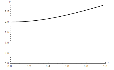
We illustrate the nature of our methodology by considering the elementary case of the planar single-input triangular system x˙1=x2u,x˙2=x1x23{{{\dot{x}}}_{1}}={{x}_{2}}u,{{{\dot{x}}}_{2}}={{x}_{1}}-x_{2}^{3} with output y=x1y={{x}_{1}} that has the form (3.1) with

A:=[0u00]and f:=(0,x1x23).A:=\left[\begin{matrix}0&u\\ 0&0\\ \end{matrix}\right]\text{and }f:=\left(0,{{x}_{1}}-x_{2}^{3}\right)^{\prime}.

We may assume that each admissible input uu is any nonzero measurable and essentially locally bounded function and for simplicity, let u(t)=1u(t)=1 for tt near zero. Obviously, the system above satisfies H1 and H2. Let us choose (x1(0),x2(0))=(2, 0)({{x}_{1}}(0),{{x}_{2}}(0))=(2,\,0) as initial condition and calculate the corresponding output trajectory y=x1y={{x}_{1}} (see Figure 1 below).

Figure 1: Output of the System
Refer to caption

We next apply the methodology suggested in the previous section, in order to confirm that our proposed algorithm converges to x(0)=(x1(0),x2(0))x(0)=({{x}_{1}}(0),{{x}_{2}}(0)) above. For simplicity, let us assume that is a priori known that the “unknown” initial state x(0)x(0) is contained into the ball BR{{B}_{R}} of radius R=3R=3 centered at zero. We take R1=3,R2=6,R3=12,R4=24,R5=48,{{R}_{1}}=3,{{R}_{2}}=6,{{R}_{3}}=12,{{R}_{4}}=24,{{R}_{5}}=48,\ldots and =0.5\ell=0.5 as in the proposed algorithm (Case I). By taking into account the known values of y()y(\cdot), we find a decreasing sequence {tν}\left\{{{t}_{\nu}}\right\} satisfying (2.31) converging to t0=0t_{0}=0; particularly, take t1=5×10⁴{{t}_{1}}=5\times{{10}^{-4}} t2=1.3×10⁴,t3=3.2×10⁵,t4=7.8×10⁶,t5=1.9×10⁶,{{t}_{2}}=1.3\times{{10}^{-4}},\ {{t}_{3}}=3.2\times{{10}^{-5}},\ {{t}_{4}}=7.8\times{{10}^{-6}},\ {{t}_{5}}=1.9\times{{10}^{-6}},\ldots. Then, choose an arbitrary constant initial map, say z1()=(z11(),z12()){{z}_{1}}(\cdot)=(z_{1}^{1}(\cdot),z_{1}^{2}(\cdot)); with z11(t)=0z_{1}^{1}\left(t\right)=0 and z12(t)=1z_{1}^{2}\left(t\right)=1, for t[t0=0,t1=5×10⁴]t\in[{{t}_{0}}=0,{{t}_{1}}=5\times{{10}^{-4}}] and successively apply (2.22b), in order to evaluate the desired sequence {zν(tν):=(zν1(tν),zν2(tν)},ν=1,2,\left\{{{z}_{\nu}}({{t}_{\nu}}):=(z_{\nu}^{1}({{t}_{\nu}}),z_{\nu}^{2}({{t}_{\nu}})\right\},\nu=1,2,\ldots. Figures 2 and 3 present the corresponding values of errors eν1(tν):=zν1(tν)x1(0),eν2(tν):=zν2(tν)x2(0),ν=1,2,e_{\nu}^{1}({{t}_{\nu}}):=z_{\nu}^{1}({{t}_{\nu}})-{{x}_{1}}(0),e_{\nu}^{2}({{t}_{\nu}}):=z_{\nu}^{2}({{t}_{\nu}})-{{x}_{2}}(0),\nu=1,2,\ldots and confirms that the evaluated pair of terms zν(tν){{z}_{\nu}}\left({{t}_{\nu}}\right) converges to the pair (x1(0),x2(0))=(2,0)({{x}_{1}}(0),{{x}_{2}}(0))=(2,0).

Figure 2: Error eν1e_{\nu}^{1}
Refer to caption
Figure 3: Error eν2e_{\nu}^{2}
Refer to caption

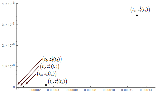
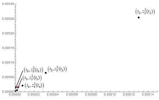
Finally, we remark that, since the system is forward complete, then for any T>t0T>{{t}_{0}} the sequence of mappings Xν(0,y,u):=x(t;0,ξν,u),t[0,T],ν=1,2,{{X}_{\nu}}(0,y,u):=x(t;0,{{\xi}_{\nu}},u),t\in[0,T],\nu=1,2,\ldots with ξν:=zν(tν){{\xi}_{\nu}}:={{z}_{\nu}}\left({{t}_{\nu}}\right) uniformly approximates the unknown solution x(;0,x(0),u)x(\cdot;0,x(0),u) on the interval [t0,T][{{t}_{0}},T].

IV Additional Hypotheses and Hybrid Observer

In this section we briefly present a hybrid-observer technique for the state estimation for (1.1). The proof of the following proposition is based on a modification of the approach employed in Section II.

Proposition IV.1

For the system (1.1) we make the same assumptions with those imposed in statement of Proposition 2.1. Also, assume that for any t0I{{t}_{0}}\in I and input uU[t0,+)u\in{{U}_{[{{t}_{0}},+\infty)}} there exists a constant C>0C>0 such that

|f(t,y,z1,u(t))f(t,y,z2,u(t))|C|z1z2|,\displaystyle\left|f\left(t,y,{{z}_{1}},u(t)\right)-f\left(t,y,{{z}_{2}},u(t)\right)\right|\leq C\left|{{z}_{1}}-{{z}_{2}}\right|,
(t,y)[t0,)×,z1,z2n\displaystyle\forall(t,y)\in[t_{0},\infty)\times\mathbb{R},{{z}_{1}},{{z}_{2}}\in\mathbb{R}^{n} (4.1)

Then, there exists a sequence ξν=ξν(t0,y,u)n,ν=0,1,2,\xi_{\nu}=\xi_{\nu}(t_{0},y,u)\in\mathbb{R}^{n},\nu=0,1,2,\ldots such that, if for any arbitrary constant h>t0h>t_{0} we define:

ω0(ξ):=ξ;ων+1(ξ)=x(t0+(ν+1)σ;t0+νσ,ων(ξ),u),ν=0,1,2,\displaystyle\begin{aligned} {{\omega}_{0}}(\xi):=\xi;\\ {{\omega}_{\nu+1}}(\xi)=x({{t}_{0}}+(\nu+1)\sigma;{{t}_{0}}+\nu\sigma,{{\omega}_{\nu}}(\xi),u),\nu=0,1,2,\ldots\end{aligned} (4.2a)
m0:=ω0(ξ0)(=ξ0);mν:=ων(ξν),ν=1,2,\displaystyle{{m}_{0}}:={{\omega}_{0}}({{\xi}_{0}})(={{\xi}_{0}});\ {{m}_{\nu}}:={{\omega}_{\nu}}({{\xi}_{\nu}}),\nu=1,2,\ldots (4.2b)

where σ:=ht0\sigma:=h-t_{0}, then the system below exhibits the global state estimation of (1.1):

x^˙(t)=A(t,y,u)x^+f(t,y,x^,u),t[t0+νσ,t0+(ν+1)σ)\dot{\hat{x}}\left(t\right)=A(t,y,u)\hat{x}+f(t,y,\hat{x},u),\ t\in\left[{{t}_{0}}+\nu\sigma,{{t}_{0}}+(\nu+1)\sigma\right) (4.3a)
x^(t0+νσ)=mν,ν=0,1,2,\hat{x}\left({{t}_{0}}+\nu\sigma\right)={{m}_{\nu}},\ \nu=0,1,2,\ldots (4.3b)

particularly, it holds:

limt|x^(t;t0,m0,u)x(t;t0,x0,u)|=0\displaystyle\underset{t\to\infty}{\mathop{\lim}}|\hat{x}(t;t_{0},m_{0},u)-x(t;t_{0},x_{0},u)|=0 (4.4)
Proof:

Let x()=x(;t0,x0,u),t0Ix(\cdot)=x(\cdot;{{t}_{0}},{{x}_{0}},u),{{t}_{0}}\in I be a solution of (1.1) corresponding to u()u(\cdot). Let h>t0h>{{t}_{0}} and consider the sequence Cν:=(exphC)ν+1,ν=1,2,{{C}_{\nu}}:={{(\exp hC)}^{\nu+1}},\nu=1,2,\ldots, with CC as defined in (4.1), and let {ν},ν(0,1/2],ν=1,2,\left\{{{\ell}_{\nu}}\right\},{{\ell}_{\nu}}\in(0,1/2],\nu=1,2,\ldots be a decreasing sequence with

limνν1Cν=0\displaystyle\lim_{\nu\to\infty}\ell_{\nu-1}C_{\nu}=0 (4.5)

We next proceed by using a generalization of the procedure employed for the proof of Proposition 2.1. First, we find a decreasing sequence tν(t0,h]{{t}_{\nu}}\in({{t}_{0}},h], ,ν=0,1,2,,\nu=0,1,2,\ldots with tνt0{{t}_{\nu}}\to{{t}_{0}} such that

tν(;t0,y,d1,u)tν(;t0,y,d2,u)[t0,tν]νd1d2[t0,tν],d1,d2C0([t0,tν];n):max{di[t0,tν],i=1,2}Rν,ν=k,k+1,k+2,\|{{\mathcal{F}}_{{{t}_{\nu}}}}(\cdot;{{t}_{0}},y,{{d}_{1}},u)-{{\mathcal{F}}_{{{t}_{\nu}}}}(\cdot;{{t}_{0}},y,{{d}_{2}},u){{\|}_{[{{t}_{0}},{{t}_{\nu}}]}}\leq{{\ell}_{\nu}}\|{{d}_{1}}-{{d}_{2}}{{\|}_{[{{t}_{0}},{{t}_{\nu}}]}},\\ \forall{{d}_{1}},{{d}_{2}}\in{{C}^{0}}\left([{{t}_{0}},{{t}_{\nu}}];{{\mathbb{R}}^{n}}\right):\max\left\{\|{{d}_{i}}{{\|}_{[{{t}_{0}},{{t}_{\nu}}]}},i=1,2\right\}\leq{{R}_{\nu}},\\ \nu=k,k+1,k+2,\ldots (4.6)

with {Rν}\left\{{{R}_{\nu}}\right\} and kk as defined by (2.18) and (2.19), respectively. Then, consider the sequence of mappings zν()n,ν=k,k+1,k+2,{{z}_{\nu}}(\cdot)\in{{\mathbb{R}}^{n}},\nu=k,k+1,k+2,\ldots, as precisely defined in (2.22) and again define:

ξν:=zν(tν),ν=k,k+1,{{\xi}_{\nu}}:={{z}_{\nu}}({{t}_{\nu}}),\nu=k,k+1,\ldots (4.7)

Then, as in proof of Propostion 2.1 we can show, by exploiting (4.6), that

|ξνx0|νν1k|ξkx0|,ν=k+1,k+2,\left|{{\xi}_{\nu}}-{{x}_{0}}\right|\leq{{\ell}_{\nu}}{{\ell}_{\nu-1}}\cdots{{\ell}_{k}}\left|{{\xi}_{k}}-{{x}_{0}}\right|,\forall\nu=k+1,k+2,\ldots (4.8)

We are now in a position to show (4.4). We take into account (4.1)-(4.3), (4.5), (4.8), definition of Cν{{C}_{\nu}} and consider the difference between the integral representation of the solutions of (1.1a) and (4.3a). Then, by successively applying the Gronwall - Bellman inequality, we can estimate:

x^(;t0+νσ,mν,u)x(;t0,x0,u)[t0+νσ,t0+(ν+1)σ]kk+1ν1Cν|ξ0x0|ν1Cν|ξ0x0|,ν=k+1,k+2,{{\left\|\hat{x}(\cdot;{{t}_{0}}+\nu\sigma,{{m}_{\nu}},u)-x(\cdot;{{t}_{0}},{{x}_{0}},u)\right\|}_{[{{t}_{0}}+\nu\sigma,{{t}_{0}}+(\nu+1)\sigma]}}\\ \leq{{\ell}_{k}}{{\ell}_{k+1}}\cdots{{\ell}_{\nu-1}}{{C}_{\nu}}\left|{{\xi}_{0}}-{{x}_{0}}\right|\leq{{\ell}_{\nu-1}}{{C}_{\nu}}\left|{{\xi}_{0}}-{{x}_{0}}\right|,\\ \nu=k+1,k+2,\ldots (4.9)

and the above, in conjunction with (4.5), asserts that

limνx^(;t0+νσ,mν,u)x(;t0,x0,u)[t0+νσ,t0+(ν+1)σ]=0\underset{\nu\to\infty}{\mathop{\lim}}\,{{\left\|\hat{x}(\cdot;{{t}_{0}}+\nu\sigma,{{m}_{\nu}},u)-x(\cdot;{{t}_{0}},{{x}_{0}},u)\right\|}_{[{{t}_{0}}+\nu\sigma,{{t}_{0}}+(\nu+1)\sigma]}}=0

The latter implies the desired (4.4). Details are left to the reader. ∎

V Conclusion

Sufficient conditions for observability and solvability of the state estimation for a class of nonlinear control time - varying systems are derived. The state estimation is exhibited by means of a sequence of functionals approximating the unknown state of the system on a given bounded time interval. Each functional is exclusively dependent on the dynamics of system, the input uu and the corresponding output yy. The possibility of solvability of the state estimation problem by means of hybrid observers is briefly examined.

References

  • [1] T. Ahmed-Ali and F. Lamnabhi-Lagarrigue, “Sliding observer-controller design for uncertain triangular nonlinear systems,” IEEE Transactions on Automatic Control, vol. 44, no. 6, pp. 1244–1249, 1999.
  • [2] J. H. Ahrens and H. K. Khalil, “High-gain observers in the presence of measurement noise,” Automatica, vol. 45, no. 4, pp. 936–943, 2009.
  • [3] M. Alamir, “Optimization based non-linear observers revisited,” International Journal of Control, vol. 72, no. 13, pp. 1204–1217, 1999.
  • [4] A. Alessandri and A. Rossi, “Increasing-gain observers for nonlinear systems: Stability and design,” Automatica, vol. 57, pp. 180–188, 2015.
  • [5] V. Andrieu, L. Praly, and A. Astolfi, “High gain observers with updated gain and homogeneous correction terms,” Automatica, vol. 45, no. 2, pp. 422–428, 2009.
  • [6] A. Astolfi and L. Praly, “Global complete observability and output-to-state stability imply the existence of a globally convergent observer,” Mathematics of Control, Signals, and Systems, vol. 18, no. 1, pp. 32–65, 2006.
  • [7] G. Besançon and A. Ticlea, “An immersion-based observer design for rank-observable nonlinear systems,” IEEE Transactions on Automatic Control, vol. 52, no. 1, pp. 83–88, 2007.
  • [8] D. Boskos and J. Tsinias, “Sufficient conditions on the existence of switching observers for nonlinear time-varying systems,” Eur. J. Control, vol. 19, pp. 87–103, 2013.
  • [9] ——, “Observer Design for Nonlinear Triangular Systems with Unobservable Linearization,” International Journal of Control, vol. 86, pp. 721–739, 2013.
  • [10] ——, “Observer Design for a General Class of Triangular Systems,” Proc. 21st Symp. Math. Theory Netw. Syst. (MTSN), 2014.
  • [11] H. Du, C. Qian, S. Yang, and S. Li, “Recursive design of finite-time convergent observers for a class of time-varying nonlinear systems,” Automatica, vol. 49, no. 2, pp. 601–609, 2013.
  • [12] P. Dufour, S. Flila, and H. Hammouri, “Observer design for MIMO non-uniformly observable systems,” IEEE Transactions on Automatic Control, vol. 57, no. 2, pp. 511–516, 2012.
  • [13] J. P. Gauthier, H. Hammouri, and S. Othman, “A Simple Observer for Nonlinear Systems Applications to Bioreactors,” IEEE Transactions on Automatic Control, vol. 37, no. 6, pp. 875–880, 1992.
  • [14] J.-P. Gauthier and I. Kupka, Deterministic Observation Theory and Applications. Cambridge: Cambridge University Press, 2001.
  • [15] T. Hoàng, W. Pasillas-Lépine, and W. Respondek, “A switching observer for systems with linearizable error dynamics via singular time-scaling,” Proc. 21st Symp. Math. Theory Netw. Syst. (MTNS), 2014.
  • [16] I. Karafyllis and Z. P. Jiang, “Hybrid dead-beat observers for a class of nonlinear systems,” Systems and Control Letters, vol. 60, no. 8, pp. 608–617, 2011.
  • [17] I. Karafyllis and C. Kravaris, “Global exponential observers for two classes of nonlinear systems,” Systems and Control Letters, vol. 61, no. 7, pp. 797–806, 2012.
  • [18] D. Karagiannis, M. Sassano, and A. Astolfi, “Dynamic scaling and observer design with application to adaptive control,” Automatica, vol. 45, no. 12, pp. 2883–2889, 2009.
  • [19] N. Kazantzis and C. Kravaris, “Nonlinear observer design using Lyapunov’s auxiliary theorem,” Proceedings of the 36th IEEE Conference on Decision and Control, vol. 5, no. June 1997, pp. 241–247, 1997.
  • [20] J. Klamka, “On the global controllability of perturbed nonlinear systems,” IEEE Trans. Automat. Control 20 (1), pp. 170–172, 1975.
  • [21] A. J. Krener and M. Xiao, “Observers for linearly unobservable nonlinear systems,” Systems and Control Letters, vol. 46, no. 4, pp. 281–288, 2002.
  • [22] P. Krishnamurthy and F. Khorrami, “Dynamic High-Gain Scaling: State and Output Feedback With Application to Systems With ISS Appended Dynamics Driven by All States,” IEEE Trans. Autom. Control, vol. 49, no. 12, pp. 2219–2239, 2004.
  • [23] T. Ménard, E. Moulay, and W. Perruquetti, “Global finite-time observers for non linear systems,” in Proceedings of the IEEE Conference on Decision and Control, 2009, pp. 6526–6531.
  • [24] H. Ríos and A. R. Teel, “A hybrid observer for fixed-time state estimation of linear systems,” in 2016 IEEE 55th Conference on Decision and Control (CDC), Las Vegas, NV, 2016, pp. 5408–5413.
  • [25] D. Theodosis, D. Boskos, and J. Tsinias, “Observer design for triangular systems under weak observability assumptions,” IEEE Transactions on Automatic Control, 2018.
  • [26] J. Tsinias, “Links between asymptotic controllability and persistence of excitation for a class of time-varying systems,” Systems and Control Letters, vol. 54, no. 11, pp. 1051–1062, 2005.
  • [27] ——, “Time-varying observers for a class of nonlinear systems,” Syst. Control Lett., vol. 57, no. 12, pp. 1037–1047, 2008.
  • [28] J. Tsinias and D. Theodosis, “Luenberger-type observers for a class of nonlinear triangular control systems,” IEEE Trans. Autom. Control, vol. 61, no. 12, pp. 3797–3812, 2016.
  • [29] Y. Yamamoto and I. Sugiura, “Some sufficient conditions for the observability of nonlinear systems,” J. Optim. Theory Appl., vol. 13, no. 6, pp. 660–669, 1974.