Observability of 2HDM Neutral Higgs Bosons in fully hadronic decay at future linear collider
Abstract
The study aims to investigate the observability of pseudoscalar Higgs boson and neutral heavy CP even Higgs boson , at different benchmark points, in the framework of type-I 2HDM. The study is done for collisions at = 1000 GeV centre of mass energy (c.o.m.) a possible scenario in future lepton collider. The associated production of and in collisions are investigated in fully hadronic final state in two different channels. The first one is while the other one is . The observability of neutral heavy Higgs and pseudoscalar Higgs signal is possible within the parameter space which satisfies all experimental and theoretical constraints. The CP odd and CP even Higgs bosons in all scenarios are observable when signal exceeds , which is the final extracted value of signal significance. The signal significance is calculated at different integrated luminosities. It is concluded from current analysis that fully hadronic channel is promising for search and measurement of the neutral Higgs Bosons in 2HDM.
pacs:
12.60.Fr, 14.80.FdI Introduction
After the decades of continuous searches, the Standard Model (SM) Higgs boson was discovered by the CMS and ATLAS experiments at the Large Hadron Collider (LHC) in 2012. This proved to be the corner stone in a very successful theory which passed all of the experimental tests. Yet there are a number of reasons which lead us to believe that this is at best an incomplete theory. This opens a way for physics that is beyond the standard model BSM. The BSM comprises of many theories, but to establish any of these, the experimental evidence is required. The Two Higgs Doublet Model 2HDM is a model that provides a simple extension to the standard model and features in a number of BSM theories including the Minimal Supersymmetric Standard Model MSSM. There are eight degrees of freedom in two doublet model out of which three degrees of freedom are eaten up by the electroweak bosons due to electro-weak symmetry breaking. The remaining five degrees of freedom lead to five physical Higgs bosons that are 2 CP CP-even neutral scalar Higgs bosons , , a CP-odd pseudoscalar neutral Higgs boson and a pair of charged Higgs bosons . The existence of these Higgs bosons are to be verified through experimental measurements of production cross sections and branching ratios. In July 2017, ATLAS published the results for collaboration on the trending search of decaying neutral Higgs collaboration into two tau leptons. The tau leptons are individually interesting to search due to the existence of strong coupling of A/H and fermions of down type for the specific value of MSSM provided parameter space. These will certainly boost up the probability of A/H production in accordance with b-quarks and provides a higher cross-section. Future lepton collider such as will play an important role for the detection of Higgs boson. The precise attention is given to search the Higgs boson. The main focus of this study is to investigate the production of neutral Higgs in association to at electron positron collider. The assumed framework for the study is Type 1 2HDM. Several benchmark points are assumed with different mass hypotheses. Two decay channels are investigated in this study. In the first one, the pseudoscalar Higgs decays to boson along with neutral CP even heavy Higgs boson , the Z boson then decays hadronically to quarks while the H boson decays to leading to two light jets and four b jets in final state (). The Feynman diagram for first process is given in Figure 1.
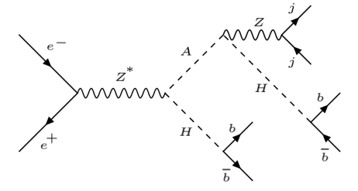
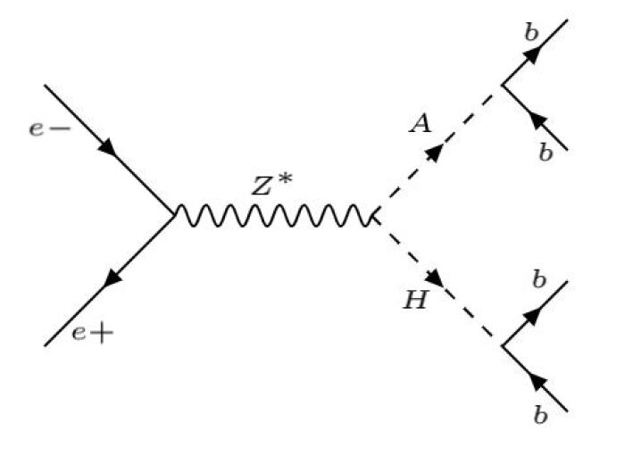
In the second decay channel both A and H decay to b-quarks leading to four b jets in final state (). The Feynman diagram of this process is given in Figure 2.
II Two Higgs Doublet Model 2HDM
The 2HDM is extension of the SM which is featured in many BSM theories. This model is proficient in solving some of the problems in SM while still maintaining the good agreement between the SM and experiments. The 2HDM offers the most simple extension of the SM where the Higgs sector is extended by including an additional doublet in the theory. The Supersymmetric theories show that the scalars are associated to chiral multiplets and opposite chirality is found in their complex conjugates. The most attractive feature of 2HDM that it smoothens the way for initiating new possibilities for explicit or for the automatic CP violation fk . Each class of 2HDM gives interesting environment and unique phenomenology. The 2HDM is divided into four types depending on the coupling of fermions with the doublets as shown in Table 1.
| Types of Model | Description | Up quarks | Down quarks | charged leptons |
|---|---|---|---|---|
| Type I | Fermiophobic | |||
| Type II | MSSM like | |||
| X | Lepton-specific | |||
| Y | Flipped |
General scalar of 2HDM is the most usual scalar potential of 14 parameters which can function as charge parity (CP) conserving, parity-violating and charge violating minima. The common scalar potential expression is assumed for two doublets and gf with hypercharge +1 and is given in equation (1)
| (1) | |||
This potential contains all real parameters with two assumed doublets in 2HDM. and are the values of vacuum expectation of two doublets i.e and . The doublet expanded by making known to eight read field , , all over the place of these minima, is given in equation (2)
| (2) |
| (3) |
By implementing the two minimization conditions of 2HDM, the terms and can be eliminated in the favour of pseudo scalar inputs. By the use of conditions seven real independent parameters are obtained.
To be more convenient, the other parameters would be . Where is mixing angle which rotates non-physical states ( and ) to the physical states ( and ). For Yukawa Lagrangian, the procedure as in SM cannot be followed and if both of the Higgs doublets couples to SM fermions, this would be flavor violating. To overcome this problem, the discrete symmetry is imposed.
A discrete symmetry gs was forced on the 2HDM potential to avoid FCNCs ga but the potential still contains a term that clearly breaks this symmetry. If is not disappearing, the potential is not invariant under the transformation but this form of symmetry breaking is only soft because has mass dimension.
The constraints are applied to 2HDM parameters by some of the theoretical considerations like perturbativity, vacuum stability, perturbative unitarity. Consistency is checked at the confidence level of .
III Signal Process
The observability of neutral Higgs bosons is investigated in two final states. In the first one we have signal chain process and in second final state the chain process is within framework of Type 1 2HDM in the low regime and enhancement of and is achieved. The boson goes into hadronic decay as a di-jet pairs , . The enhancement of the Higgs boson decay mode is due to factor. The several benchmark points with different mass hypothesis are shown in Table 2. At linear collider, the initial collision is assumed to take place at the centre of mass energy GeV and integrated luminosity is assumed to be 500 . The range for mass of the CP-even Higgs boson is assumed to be from GeV and for CP-odd Higgs boson , the assumed range is GeV with the mass splitting of in all the scenarios. The value of is set to for all scenarios which results in the enhancement of H decay. To satisfy theoretical requirement of potential stability sp , there is a range of parameter for each scenario. By using 2HDMC-1.7.0 con , perturbativity and unitarity constraints are checked.
Branching ratios (BR) are achieved by using 2HDMC-1.7.0 con . B-tagging and jet reconstruction algorithms give rise in the uncertainties which perturb the final results due to more errors in the hadronic boson decay. The boson decay provides a simple and clean signature at linear collider. The branching ratio of hadronic decay of boson is BR and the BR for decay is BR . In process, the and Higgs boson are reconstructed by recombination of two light-jets and two b-jets respectively. The pseudoscalar Higgs boson is then reconstructed by the reconstructed and bosons. In the second process, both and are reconstructed by recombination of b-jet pairs.
The main SM background processes which are taken into account for this analysis, relevant to signal are pair production of di-vector boson , , top quark and production. Cross sections are computed at GeV by PYTHIA 8.2.10 pythia1 and are given in Table 2. The cross section for first process is represented by and for second process it is represented by
| BP1 | BP2 | BP3 | BP4 | |||||
| 125 | 125 | 125 | 125 | |||||
| 150 | 200 | 250 | 300 | |||||
| 250 | 300 | 330 | 400 | |||||
| 250 | 300 | 330 | 400 | |||||
| 1987-2243 | 3720-3975 | 5948-6203 | 8671-8925 | |||||
| 10 | 10 | 10 | 10 | |||||
| 1 | 1 | 1 | 1 | |||||
| at GeV | 10.16 | 8.211 | 6.675 | 4.213 | 3192 | 210.8 | 69.24 | 2328 |
| at GeV | 5.587 | 5.137 | 4.725 | 3.937 | 1812 | 102.6 | 38.92 | 1063 |
| at GeV | 1.692 | 1.625 | 1.603 | 1.484 | 687.5 | 28.94 | 13.79 | 278.8 |
| at GeV | 10.16 | 8.221 | 6.686 | 4.212 | 3192 | 211.4 | 109.3 | 2874 |
| at GeV | 5.609 | 5.090 | 4.694 | 4.001 | 1815 | 101.8 | 61.38 | 1320 |
| at GeV | 1.681 | 1.628 | 1.59 | 1.48 | 687.2 | 28.89 | 21.59 | 347.6 |
The Branching Ratio for decay of neutral Higgs boson H into bottom quark pairs for our assumed BP points are calculated by using 2HDMC-1.7.0. Branching ratios of heavy neutral Higgs bosons H and pseudo scalar A Higgs boson decay for different benchmark points are tabulated in the Table 3 and Table 4 respectively.
| BP | |||
|---|---|---|---|
| BP | ||||
|---|---|---|---|---|
IV EVENT GENERATION, SIGNAL SELECTION AND ANALYSIS
The parameters of Type-1 are produced in SLHA (SUSY Les Houches Accord) format by using 2HDMC-1.7.0 con . This output file is passed to PYTHIA 8.2.10 pythia1 to generate the events. The generated particles in each event are then passed to clustering algorithm fastjet-3.3.3 to make jets mm . In order to record the events data, the interface of HepMC-2.06.06 Hep is given to Pythia. The output of Pythia is then analyzed and histograms are plotted by using Root- 6.20/04 root .
Different kinematic selection cuts are applied which arises certain fluctuations in the signal. These cuts define the band of ranges which are invariant quantities, measured in events. It must fulfil the number of several final state particles. These particles are identified in phase of primary reconstruction using “object identification cuts”. Then the kinematic selection cuts are applied to refine the rejection and selection of background events to finalise the results.
The first step in event selection is the kinematic cut on jets which omit the soft jets and the ones that are in forward region along the collision beams. For this we apply following cuts on transverse momentum and pseudorapidity of jets.
| (4) |
Once we have jets within the desired kinematic range, we split the reconstructed jets by identifying them as light and b-tagged jets. In order to achieve this, we do a matching of the jets with the generated particles which is defined as
| (5) |
We identify the jets which are within of the b-quarks in the event as b-jets and the ones that are farther away from b-quarks as light jets. Once we have identified the jets, we apply the multiplicity cut on the jet. For channel we require the event to have at least two light jets and at least four b-jets while for we require at least 4 b-tagged jets.
In analysis, we use the selected light-jets (b-jets) for find a combination that minimise the defined as follows.
| (6) |
where are the dijet mass, is the mass of boson, and is the mass of the heavy Higgs boson according to the BP taken, and the are the widths of the respective mass distributions. The cut of is applied to select only events with good reconstructed and bosons. The pseudoscalar Higgs boson is then reconstructed using the combination of and which gives mass nearest to nominal mass according to the BP.
The same treatment is given to analysis but in this case, is defined as
| (7) |
After applying different selections cuts, The efficiencies are calculated for different benchmark points and are given in Table 5 for first process and Table 6 for second process respectively.
| Cuts | BP 1 | BP 2 | BP 3 | BP 4 |
| Two light jets | 0.4078 | 0.5122 | 0.5072 | 0.6249 |
| Four b-jets | 0.5945 | 0.6364 | 0.6270 | 0.6496 |
| 0.6356 | 0.5271 | 0.2910 | 0.3408 | |
| Total Efficiency | 0.1541 | 0.1718 | 0.09254 | 0.1384 |
| x BR[] | 4.481 | 2.886 | 1.715 | 0.580 |
| Cuts | BP 1 | BP 2 | BP 3 | BP4 |
| Four b-jets | 0.7161 | 0.7221 | 0.7167 | 0.7059 |
| 0.7764 | 0.6766 | 0.6036 | 0.5053 | |
| 0.8118 | 0.8013 | 0.8024 | 0.8207 | |
| Total Efficiency | 0.4514 | 0.3915 | 0.3471 | 0.29 |
| x BR[] | 4.09042 | 2.94312 | 6.79966 | 4.74 |
V RESULT AND DISCUSSION
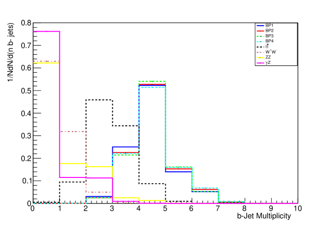
In the finalized results, topology of our assumed first signal process contains four b-jets and two light jets. The distribution of b-jet multiplicity for process having 4 bjets and 2 light jets is depicted in Figure 3 .
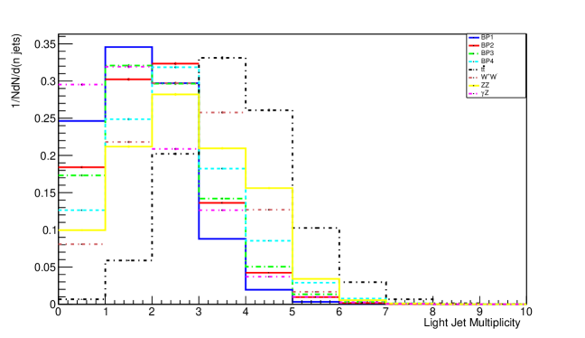
More than 60 percent of the jets are passed through the jets kinematic cut. The distribution of light jet multiplicity for this process is shown in Figure 4 for both background and signal events.
The other process contains 4 b-jets. The distribution of b-jet multiplicity for this process is shown in Figure 5 .
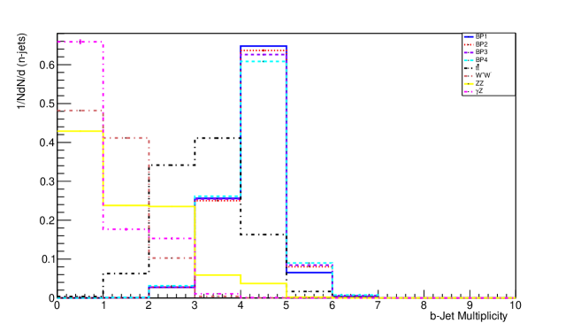
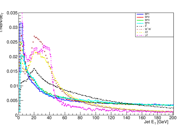
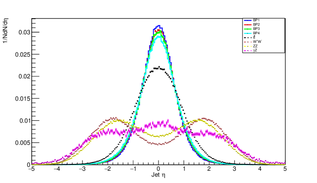
The distribution of b-jets slightly depends on neutral Higgs boson mass in the assumed signal event. The production of b-jet is suppressed kinematically in the production of Higgs boson, the availability of phase space is smaller due to which it decays to bottom quarks. Transverse energy of jets for second process is shown in figure 6.
The pseudorapidity of jets for this process is shown in figure 7.
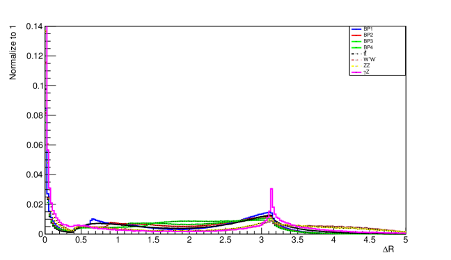
After extracting out the data of , the profiling process of is discussed. By the analysis of plot of shown in Figure 8, the b-jets can easily be identified by finding the minima of the plot.
For all the distribution profiles, the implemented integrated luminosity is . The cross-sections of the signal are collected by multiplying the branching ratios with corresponding total cross-sections and are given in Table 5 for first process and in Table 6 for second process.
V.1 Mass reconstruction
The invariant mass of neutral scalar Higgs bosons is reconstructed. In this work, the generation of signal and background processes is involved which display natural interference and selection techniques where different mass speculations are displayed for Higgs invariant mass remaking.
The process of mass reconstruction of Higgs bosons is considered as important to attain the reliable separation between the main assumed signal and the background processes. Peak of the signal resonance would be produced by the proper mass variable. By this process, large signal will be produced over the background ratio. The pair of b-jets comes out from the heavy Higgs Boson in the signal events. Due to that fact, the invariant mass of this pair should be lesser and lie within mass casement adjusted by neutral Higgs mass. Mass of the Higgs Boson can be calculated by the conventional formula given as
| (8) |
VI Chi-square method
Chi-square test is based on comparing observed and expected values. This test is designed to determine whether a difference between actual and predicted data is due to chance or due to relationship between the variables under consideration. As a result, Chi-square test is a fantastic tool for analyzing and understanding the relationships between our categorical data. The Chi-square method is used in this study to compare the reconstructed and actual values of Higgs boson mass. To determine the best estimate of Higgs-boson mass, I minimized the appropriately weighted sum of squared differences between observed and predicted values, known as ”Chi-square”. The general formula for Higgs boson is given in equation (9)
| (9) |
The reconstructed invariant mass of the Higgs boson is represented by ””, and the actual value of the Higgs boson mass is represented by ””. Then, for each possible combination, the sum of squared differences between observed and predicted Higgs-boson masses is calculated. Then, light jet and bjet pairings that meet the following conditions are chosen.
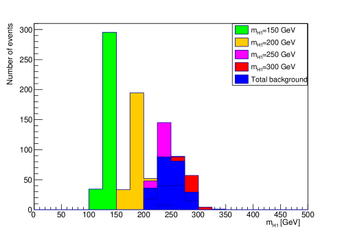
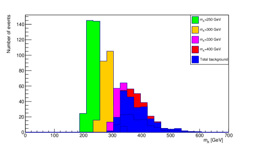
Then, using this true light jet pair, the Higgs-boson mass is reconstructed. The reconstructed invariant mass of Higgs-boson from b jet pairs and light-jet pairs for all signal along with SM backgrounds are shown in figures. The figures Figure 9 and Figure 10 represents the reconstruction of neutral scalar Higgs for first process.
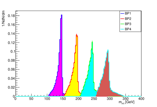
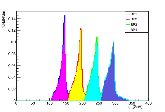
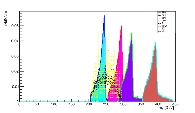
The reconstruction of neutral Higgs boson is plotted in Figure 11 for second process.
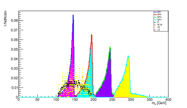
The mass peak of neutral scalar Higgs can be clearly seen in the Figure 11 which suppresses the significant background processes. From Figure 9 , Figure 10 and Figure 11 it can be examined that the attained data fall nearly to the input mass which is only possible due to the testing of different mass hypothesis of neutral scalar Higgs in simulation.
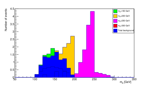
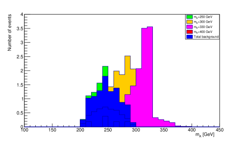
VI.1 Mass Reconstruction of Pseudo scalar Higgs
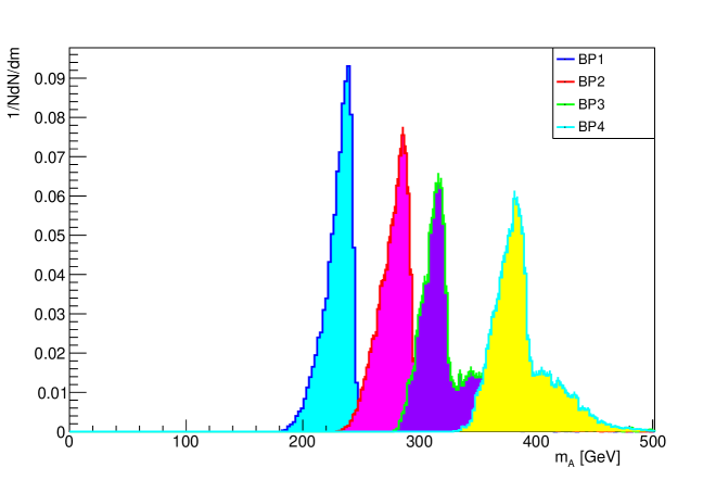
In our assumed signal process, the decay of A Higgs boson occurs as . In accordance with that scenario, the jets which successfully passes the cuts, A candidate are considered by identifying the combination of bjets. In events with possible two candidates of H, smallest value of the parameter of the combination of ZH is clearly assumed as A candidate. The plot for reconstruction of pseudo scalar Higgs A for first and second process are shown in figures Figure 12 and Figure 13 respectively.
VI.2 Mass Reconstruction of Z boson
The jets are assumed as the light jets which do not fulfill the requirements for the declaration of b-jets. For obtaining the reconstructed invariant mass of Z boson, two of the leading jets are mainly selected which have same and cuts implemented on all jets. The feature, low jet multiplicity of the signal events, is used for the suppression of the Z single events. The two light jets having the highest are fused together to create the candidate of Z-boson.
The functions which are properly fit are mainly fitted to the distributions of signal and the finalized results are indicated with the error bars. The significant peaks in the fitted profiles are near to the Higgs masses which are generated in our scenario. ROOT 6.20 root is used for the fitting process. The Gaussian function was observed in the signal distributions of fit functions. The signal was covered by the Gaussian function. To find out the central region of a signal peak the parameter “Mean” is used which is the parameter of the fit function of Gaussian. Values of the parameter Mean are assumed as reconstructed masses of Higgs bosons which are termed as . For the comparison, it also indicates the generated masses which are termed as . There is difference between the reconstructed and generated masses due to arising uncertainties, from the algorithm of jet clustering and the mis-identification of jets, rate of mis-tagging jet, method of fitting and the selection of the fit function, errors arising in the energy and the momentum of particles, etc. The error factor may be reduced by the process of optimization of the algorithm of jet clustering, the algorithm of b-tagging and the method of fitting. Generated, reconstructed and corrected reconstructed mass of neutral scalar Higgs H1 and Pseudo scalar Higgs A is shown in Table 7 and Table 8.
| BP1 | 150 | 140.30.1 | 152.860.2 |
|---|---|---|---|
| BP2 | 200 | 186.40.1 | 198.960.2 |
| BP3 | 250 | 236.50.1 | 249.060.2 |
| BP4 | 300 | 286.50.1 | 299.060.2 |
| BP1 | 250 | 229.960.16 | 243.840.43 |
|---|---|---|---|
| BP2 | 300 | 277.20.12 | 291.080.0.39 |
| BP3 | 330 | 337.80.61 | 323.920.0.88 |
| BP4 | 400 | 379.890.18 | 393.770.45 |
From Table 7 and Table 8, the average difference between the generated mass and reconstructed mass of and A is 12.56 and 13.88 respectively for first process, and average mass error is 0.1 and 0.27 respectively. This error is reduced by adding a same value in reconstructed mass and fill in column. Similarly average value of error is added in all error values and given in third column. From the Table 7 and Table 8 it is concluded that reconstructed mass is few GeV different from generated mass. Generated, reconstructed and corrected reconstructed mass of neutral scalar Higgs H and Pseudo scalar Higgs A is shown in Table 9 and Table 10.
| BP1 | 150 | 139.90.1 | 153.80.13 |
|---|---|---|---|
| BP2 | 200 | 186.50.009 | 200.40.039 |
| BP3 | 250 | 234.40.007 | 248.30.037 |
| BP4 | 300 | 283.60.007 | 297.50.0.037 |
| BP1 | 250 | 233.90.1027 | 250.950.1327 |
|---|---|---|---|
| BP2 | 300 | 282.50.008 | 299.950.038 |
| BP3 | 330 | 312.3830.007 | 329.4330.037 |
| BP4 | 400 | 3830.007 | 400.050.037 |
From Table 9 and Table 10, the average difference between the generated mass and reconstructed mass of H and A is 13.9 and 17.05 respectively for second process, and average mass error is 0.03 and 0.03 respectively. This error is reduced by adding a same value in reconstructed mass and fill in column. Similarly average value of error is added in all error values and given in third column. From the Table 7 and Table 8 it is concluded that reconstructed mass is few GeV different from generated mass.
VII Signal significance
To figure out the observability in our assumed scenario of A and H Higgs bosons, for each one of the distribution of the candidate mass, the significance of signal is computed. The numbers of candidate masses in signal and background events are counted in whole mass series. Mainly the jets are not easily detected as the b-jets due to the production of several jets in the ongoing events. In the assumed scenario, several techniques are used to identify the jets. The associated jets are identified through the process of tagging which is aptly known as the algorithm of b-tagging. To identify the b-jets, the minimum distance between the b-parton and all of the generated jets is calculated. The term delta R is helpful in finding out the b-jets by calculating the distance between the b-parton and the jets. The computation of significance of signal is totally based on the luminosity (Integrated) of 100 , 500 , 1000 and 5000 for all of our profiles of mass distribution. The Table 11 shows the signal significance values at each benchmark point, for neutral Higgs H in first process at integrated luminosities of , , and and total efficiency.
| BP1 | BP2 | BP3 | BP4 | |
| Significance S/ at | 2. 74433 | |||
| Significance S/ at | 6.13 | |||
| Significance S/ at | 8.80 | 8.6 | ||
| Significance S/ at | 19.40 | |||
| at = 100 | 0.1541 | 0.168993 | 0.0785 | 0.11 |
| at = 500,1000,5000 | 0.1541 | 0.168993 | 0.080 | 0.11 |
Table 12 shows the signal significance values at each benchmark point, for Pseudo scalar Higgs A in first process at integrated luminosities of , , and and total efficiency.
| BP1 | BP2 | BP3 | BP4 | |
| Significance S/ at | 1.21 | |||
| Significance S/ at | 3.114 | |||
| Significance S/ at | 4.03 | |||
| Significance S/ at | 10.1189 | |||
| at = 100,1000 | 0.14 | 0.14 | 0.0569755 | 0.093 |
| at = 500,5000 | 0.1484 | 0.1484 | 0.0569755 | 0.13 |
Table 13 shows the signal significance values at each benchmark point, for Pseudo scalar Higgs A in second process at integrated luminosities of , , and and total efficiency for second process.
| BP1 | BP2 | BP3 | BP4 | |
|---|---|---|---|---|
| Significance S/ at | 0.078 | |||
| Significance S/ at | 0.0030 | 5.70 | 28.876 | 0.175 |
| Significance S/ at | 0.004269 | 8.066 | 40.8375 | 0.2478 |
| Significance S/ at | 1.138 | 18.036 | 91.3155 | 0.5543 |
| at = 100,500,1000 | 0.000584515 | 0.153476 | 0.336317 | 0.2927 |
| at = 5000 | 0.30916 | 0.153476 | 0.336317 | 0.2927 |
Table 14 shows the signal significance values at each benchmark point, for Neutral Higgs H in second process at integrated luminosities of , , and .
| BP1 | BP2 | BP3 | BP4 | |
| Significance S/at | 0.001382 | 3.099 | 12.60 | 0.07411 |
| Significance S/ at | 0.00309 | 6.93 | 28.1776 | 0.1657 |
| Significance S/ at | 0.004373 | 9.80064 | 39.8492 | 0.2343 |
| Significance S/ at | 1.01852 | 21.9149 | 89.1055 | 0.5240 |
| at = 100,500,1000 | 0.000633225 | 0.197228 | 0.3471 | 0.2927 |
| at = 5000 | 0.37 | 0.197228 | 0.3471 | 0.2927 |
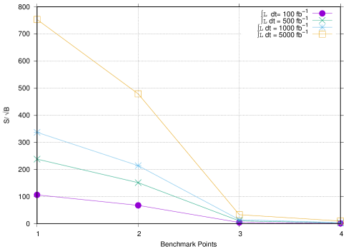
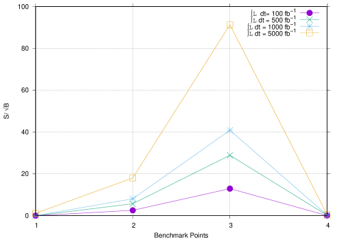
The signal significance, plotted verses benchmark points is shown in Figure 14 for first process and for second process it is shown in Figure 15.
The final results for signal significance for first and second process are shown in Figure 16, Figure 17, Figure 18 and Figure 19.
VIII Conclusion
The study aims to investigate the observability of Pseudo scalar Higgs A and Neutral scalar H in the framework of 2HDM type-I using lepton collider which will operate at center of mass energy =1000 GeV. The focus of study is Neutral Higgs pair production at electron positron collider and its fully hadronic hadronic decay. The CP even Neutral Higgs decays to pair of bottom quark and the pseudoscalar Higgs decays to Z boson along with neutral heavy CP even Higgs boson. Neutral Higgs is very unstable particle which decays in no time to pair of bottom quarks. In this work, the predicted pseudo scalar (A) and neutral scalar (H) were examined using Type-I of Two Higgs doublet model(2HDM) at SM-like scenario which is theoretical framework for this study. In 2HDM, few benchmark points (BP) in parameter space were assumed. The main chain process or the signal process is . The second process is . At low values of , possible enhancements in the couplings of Higgs-fermion may occur. At that time the chain process gives a chance for signal to take benefit from it. Even though, assumed decay (hadronic) of Z boson may arise many errors and fluctuations in the final results. The calculations due to arising uncertainties form rate of mis-tagging and the jet misidentification. Therefore enhancement of this channel completely compensates for fluctuations and errors which arise. Few benchmark points (BP) are supposed at the (center-of-mass energy) of 1000 GeV and for each BP scenario events are generated separately. By the finalized study of data, it is concluded that presented data analysis is the best way to observe and examine the whole scenario, which are assumed in this study. In the distributions of mass of the Higgs bosons, it can be seen that there exist significant amount of data and peaks in data of total background near the generated masses, in the assumed luminosities (integrated). A and H Higgs bosons in all considered scenarios are observable when signal exceeds , which is the final extracted value of signal significance in accordance with range of whole mass. Mass reconstruction was performed by the process of fitting functions to mass profiles (distributions). As a result of this process, it is concluded that in all of the assumed scenarios, the finalized reconstructed masses of Higgs bosons are in rational agreement with the generated masses and thereby Higgs bosons (A and H) mass measurements are possible. The presented analysis is expected to work like a tool for the search of predicted neutral Higgs bosons in 2HDM. Till now simulation results, center of mass(CMS) energy and the integrated luminosities are quite promising for the observation of all the assumed scenarios.
References
- (1) T. D. Lee,A theory of spontaneous T violation, Phys.Rev.D8 (1973) 1226–1239.
- (2) Abe K; et al.,Observation of Large CP Violation in the Neutral B Meson System, Phys. Rev.Lett. 87 (2001) 091802.
- (3) Elsevier.Branco, G. C.; Ferreira, P.M.; Lavoura, L.; Rebelo, M.N.; Sher, Marc; Silva, João P,Theory and phenomenology of two-Higgs doublet models, 516 (2012) . arXiv:1106.0034.
- (4) Davidson et al.,Basis-independent methods for the two-Higgs-doublet model, Phys. Rev. D 72 (2005) 035004.
- (5) S. L. Glashow et al.,Natural conservation laws for neutral currents, Phys. Rev. D 15 (1977)1958.
- (6) Anderson, S.; et al.,Branching Fraction and Photon Energy Spectrum, PhysRevLett. 87 (2001)251807.
- (7) D. Eriksson, J. Rathsman and O.Stal,2HDMC - Two-Higgs-Doublet Model Calculator., Comput. Phys. Commun. 181 (2010) 189.
- (8) M.Tanabashi et al.,Particle Data Group., Phys. Rev. D 98 (2018) 030001.
- (9) P. Bechtle, S. Heinemeyer, O. Stal, T. Stefaniak and G. Weiglein,HiggsSignals: Confronting arbitrary Higgs sectors with measurements at the Tevatron and the LHC, arXiv:1305.1933
- (10) Bechtle, Philip and Brein, Oliver and Heinemeyer, Sven and Stal, Oscar and Stefaniak, Tim and Weiglein, Georg and Williams, Karina E,HiggsBounds-4: improved tests of extended Higgs sectors against exclusion bounds from LEP, the Tevatron and the LHC., arXiv:1311.0055
- (11) Nilendra G. Deshpande and Ernest,Pattern of symmetry breaking with two Higgs doublets, Phys.Rev.D 18 (1978)2574.
- (12) Sjöstrand, Torbjörn, Stefan Ask, Jesper R. Christiansen, Richard Corke, Nishita Desai, Philip Ilten, Stephen Mrenna, Stefan Prestel, Christine O. Rasmussen, and Peter Z. Skands. ”An introduction to PYTHIA 8.2.” Computer physics communications 191 (2015): 159-177.
- (13) Cacciari, Matteo, Gavin P. Salam, and Gregory Soyez,FastJet user manual., Eur. Phys. J.C3 (2012) 1896.
- (14) The reference manual can be obtained at the URL: http://lcgapp.cern.ch/project/simu/HepMC/
- (15) The Root Reference Guide. 2013.http://root.cern.ch/drupal/content/reference- guide.https://root.cern/
- (16) ATLAS Collaboration, Expected performance of the ATLAS b-tagging algorithms in Run-2, https://cds.cern.ch/record/2037697.
- (17) Hashemi, Majid, and Gholamhossein Haghighat, Search for neutral Higgs bosons within type-I 2HDM at future linear colliders, Eur. Phys. J.C 79 (2019) 419.
- (18) Hashemi, Majid., Leptophilic neutral Higgs bosons in two Higgs doublet model at a linear collider, Eur. Phys. J.C 77 (2017) 302.
- (19) Hashemi, Majid and Haghighat ,Gholamhossein, Search for neutral Higgs bosons decaying to b b¯ in the flipped 2HDM at future linear colliders., Phys.rev.D 100 (2019) 015047.
- (20) Hashemi, Majid, and Gholamhossein Haghighat, Observability of 2HDM neutral Higgs bosons with different masses at future linear colliders., Nucl. Phys. B . 951 (2020) 114903.
- (21) Boos, Edward, et al.,CompHEP 4.4—automatic computations from lagrangians to events, Nucl. Instrum. Meth. A 534 (2004) 250-259.
- (22) Pukhov, Alexander, et al.,CompHEP-a package for evaluation of Feynman diagrams and integration over multi-particle phase space, arXiv preprint hep-ph/9908288(1999).