Observation of a non-adiabatic geometric phase for elastic waves
Abstract
We report the experimental observation of a geometric phase for elastic waves in a waveguide with helical shape. The setup reproduces the experiment by Tomita and Chiao (Phys. Rev. Lett. 57, 1986) that showed first evidence of a Berry phase, a geometric phase for adiabatic time evolution, in optics. Experimental evidence of non-adiabatic geometric has been reported in quantum mechanics. We have performed an experiment to observe the polarization transport of classical elastic waves. In a waveguide, these waves are polarized and dispersive. Whereas the wavelength is of the same order of magnitude as the helix’ radius, no frequency dependent correction is necessary to account for the theoretical prediction. This shows that in this regime, the geometric phase results directly from geometry and not from a correction to an adiabatic phase.
1 Introduction
Polarization is a feature shared by several kinds of waves: light and elastic waves, for instance, have two transverse polarization modes [1]. The polarization degrees of freedom are constrained to lie in the plane orthogonal to the direction of propagation. This constraint is responsible, in optics, for the existence of a geometric phase. Geometric phases of different kinds have been discovered after the Berry phase [2, 3, 4, 5, 6, 7, 8].
The geometric phase of light was first experimentally observed by Tomita and Chiao [9] using optical fibers. It was later suggested that a geometric phase should exist for any polarized waves [10]. This Letter discusses the case of elastic waves when the adiabatic conditions are not fulfilled, a situation which can not be reached in Optics. For polarized waves in a waveguide, the geometric phase differs from zero only if the shape of the waveguide is three-dimensional and is defined even if the time evolution is not cyclic [11].
The fundamental origin of geometric phases lies in the geometric description of the phase space. The existence of a geometric phase is related to the curvature, either local or global, of the phase space. In a first attempt to classify geometric phases, Zwanziger et al. distinguish adiabatic geometric phases [6], the main example of which is a spin in a magnetic field [2]. The geometric phase for the spin is defined if the system evolves adiabatically, such that transitions between spin states are negligible. The direction of the magnetic field must therefore evolve at a rate much smaller than the oscillation frequency between spin eigenstates.
Consider the case of waves propagating in a curved waveguide. The role of the magnetic field’s direction is played by the direction of propagation and the phase between the spin eigenstates is the orientation of the linear polarization of the wave. The adiabatic approximation imposes that the evolution rate is much smaller than the wave frequency. In the first experimental evidence for the adiabatic geometric phase, performed in optics by Tomita and Chiao [9], the frequency of light was indeed several orders of magnitude larger than . Photon spin flip is negligible, therefore the adiabaticity conditions are fulfilled. In Foucault’s pendulum [12], a renowned case of classical geometric phase, these conditions are fulfilled as well.
Some geometric phases do not require adiabaticity, such as Pancharatnam phase [13] and the Aharonov-Anandan quantum phase [4] or certain canonical classical angles [5, 14]. Geometric phases have been observed in many fields of science and called with different names. In classical mechanics, the geometric phase for adiabatic invariants is often referred to as Hannay angle [3, 15], in knot theory and DNA physics, the name writhe is mostly used [16, 17].
We consider from now on elastic waves, which polarization state can be represented as a combination of two linearly polarized states. These are classical waves, quantum transition between polarization eigenstates is not possible. The adiabaticity condition should therefore not be required to observe a geometric phase. In our experiment, indeed, the frequency and the evolution rate have the same order of magnitude. In this Letter, we briefly introduce the geometric phase in a purely geometric picture and compute its value along a helix. We present an experiment designed to measure the geometric phase of elastic waves in a helical waveguide with the condition . Without loss of generality, we only consider linear polarization.
Although the experiment we investigate has many common points with previous studies, some distinctions must be pointed out. Contrary to light polarization, the phase cannot be interpreted as a quantum phase difference between two eigenstates. There is no established classification of geometric phase but as the system we study is purely classical and neither cyclic nor adiabatic, the observed geometric phase cannot be rigorously identified as a Berry, Pancharatnam, Aharonov-Anandan or Wilczek-Zee phase, for instance. The classical geometric angles [5, 14] follow from the action-angle representation of the system, which is valid for the motion of a material point of the waveguide, but does not rigorously apply to the elastic wave transport.
2 The geometric phase for polarized waves
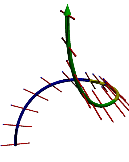
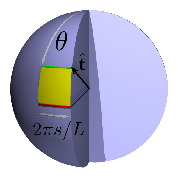
A wave travelling along a straight path keeps a constant polarization along the trajectory; if the direction of propagation is not constant, as polarization is ascribed to remain in the orthogonal plane, it evolves along the path. The path-dependent transformation transporting polarization must be, for physical reasons, linear, reversible and continuous. There is only one transformation satisfying these requirements: parallel transport [10]. Along the path followed by the wave, the direction of propagation is represented as a point on the unit sphere, polarization is represented in the tangent plane to the sphere and transported in the sphere’s tangent bundle, see Figure 1.
Let us consider a geodesic on the unit sphere, i.e. an arc of a great circle. If polarization is colinear or orthogonal to the great circle, it remains so along the geodesic to preserve symmetry. Any polarization is a linear combination of these two particular linear polarizations. The linearity of parallel transport implies, for linear polarizations, that if one rotates the initial polarization in the initial tangent plane, the parallel transported polarizations rotate by the same angle in all tangent planes of the tangent bundle. Parallel transport can be extended to any smooth and piecewise differentiable trajectory of the tangent vector on the unit sphere by discretizing the path into elementary arcs of great circles [18].
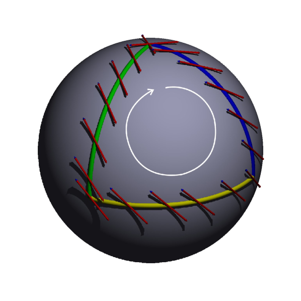
A vector parallel transported along a closed trajectory does not necessarily have the same orientation in the tangent plane at the starting point after one stride along the trajectory. The angle between the initial and final vectors is algebraically equal to the area enclosed by the trajectory on the sphere [19]. In the Figure 1, this area is equal to . It is also known as the anholonomy of the trajectory in the phase space.
3 Computation of the phase
All the distances, denoted by , are given in arclength along the helix and the accelerometers position is taken as the origin. We call the radius of the helix and its pitch, and define . The angle between the direction of propagation and the helix main axis is given by . The Frénet torsion of the helix is constant. is the azimuth angle spanned by the tangent vector along a distance on the helix. Fuller’s theorem states that the geometric phase difference between two trajectories is equal to the area spanned by the tangent vector on the unit sphere during one smooth deformation of one trajectory into the other. We chose as reference the trajectory (the limit case where the helix is a flat circle) for which it is known that the geometric phase vanishes because the trajectory is two-dimensional. After deformation of the reference into the helix, Fuller’s theorem yields a phase proportional to and the proportionality coefficient is (given by the classic geometry formula for the spherical cap area). We obtain a geometric phase of:
| (1) |
From an intrinsic point of view, parallel transport corresponds to transporting a polarization vector while keeping it constant for an imaginary walker striding along the trajectory. In the language of differential geometry the vector’s covariant derivative must equal zero along the trajectory [19]. We obtain the equation of parallel transport:
| (2) |
The components of in the Frénet-Serret frame follow a differential equation describing a rotation at the rate , leading to a phase:
| (3) |
4 Experiment
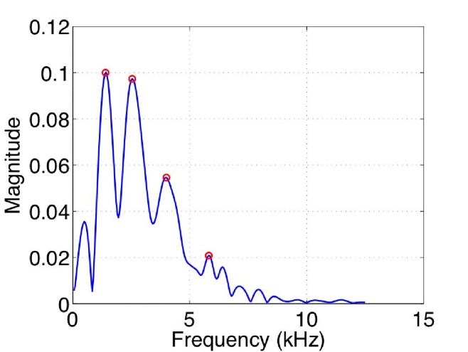
In order to reproduce the setup used by Tomita and Chiao [9], we use a metallic spring as a waveguide for elastic waves, taken from a car’s rear damper. It has a circular section of making five coils of radius and with a pitch of . The direction of propagation makes a constant angle with the helix’ main axis. As the cross-section of the helix is circular, the flexural modes are degenerated. The helix is suspended to two strings to isolate the system. We use two accelerometers (Brüel & Kjaer, type 4518-003) located at one end of the spring and record vibrations in two orthogonal directions (see Figure 3). The sampling frequency being set to , the information in the signal is available up to . Considering the accelerometers’ power spectrum in their stability range (see Figure 4), frequencies above can be ignored. The signal is amplified (Brüel & Kjaer amplifier, type 2694) before signal processing.
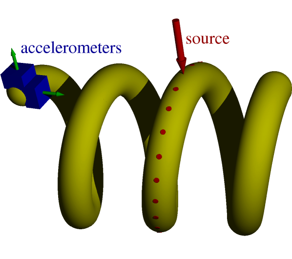
We record the waves generated by 32 equally spaced sources, which distance from the accelerometers ranges from to . Making weak impacts on the metal spring creates bending waves that are linearly polarized. Impacts are made radially with respect to the helix. The source signal is generated manually, by gently hitting the waveguide with a hammer at the different source positions. Polarization depending only on the amplitude ratio measured by the accelerometers, it is not sensitive to the energy of the source.
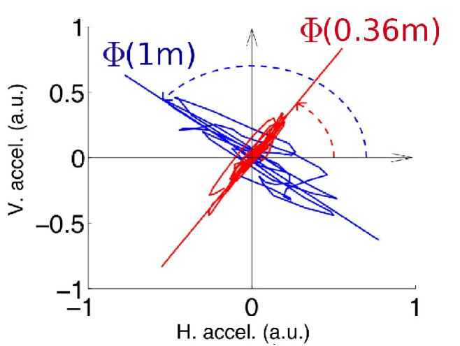
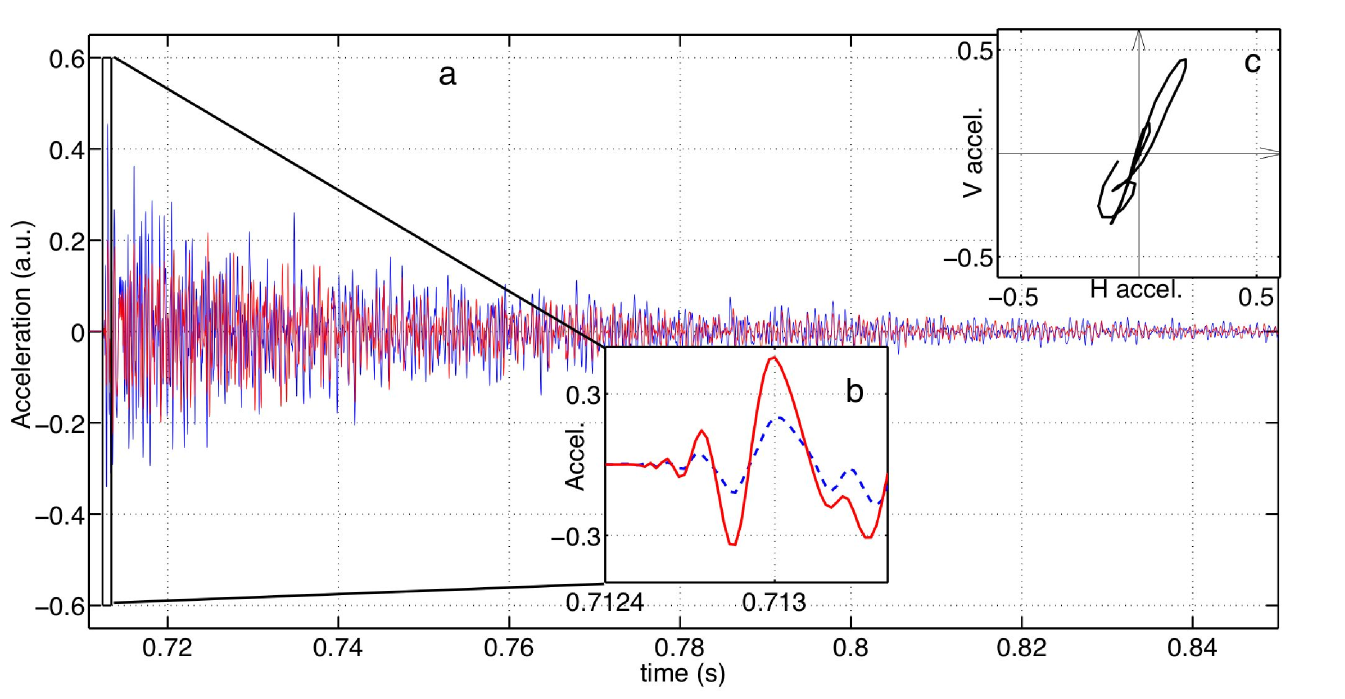
The wave propagation modes in helical waveguide constitute a difficult problem. Solutions can only be found numerically [20] and yield a complex mode structure. The fundamental mode is a flexural mode with linear polarization. Polarization losses appear rapidely after the first waveforms. In order to measure the geometric phase, we use only the first periods of oscillation of the signal, before depolarization is complete. In figure 2, the time windowed signals used for polarization orientation estimation are presented, together with the complete waveforms and associated polarization parametric plots. In Figure 4, we show an example of two parametric polarization plots for signals obtained with the source at different distances from the accelerometers. The relative angle between polarization orientations is the geometric phase difference.
Bending waves in the waveguide are dispersive. We therefore filtered the signal using non-overlapping bandpass filters centered at frequencies: , , and . These values correspond to maxima of the power spectrum displayed in figure 4 (left). The corresponding velocities are displayed in the Table 1.
The polarization orientation is obtained from the records using a principal component analysis [21]. This technique consists in obtaining the eigenvectors of the cross-correlation between the two orthogonal signals (recorded on the two accelerometers). The eigenvector with the largest eigenvalue gives the polarization direction. The geometric phase is thus the orientation of polarization measured when the source is located at distance from the accelerometers (see Figure 3).
We perform several measurements for each position of the source, in order to reduce effects of external perturbations and variations of the source signal. In our results, we observe oscillations that are due to imperfections related to the accelerometers response and setup. Denoting by the shift from orthogonality between the accelerometers and the ratio of their mechanical couplings, the principal components analysis yields:
| (4) |
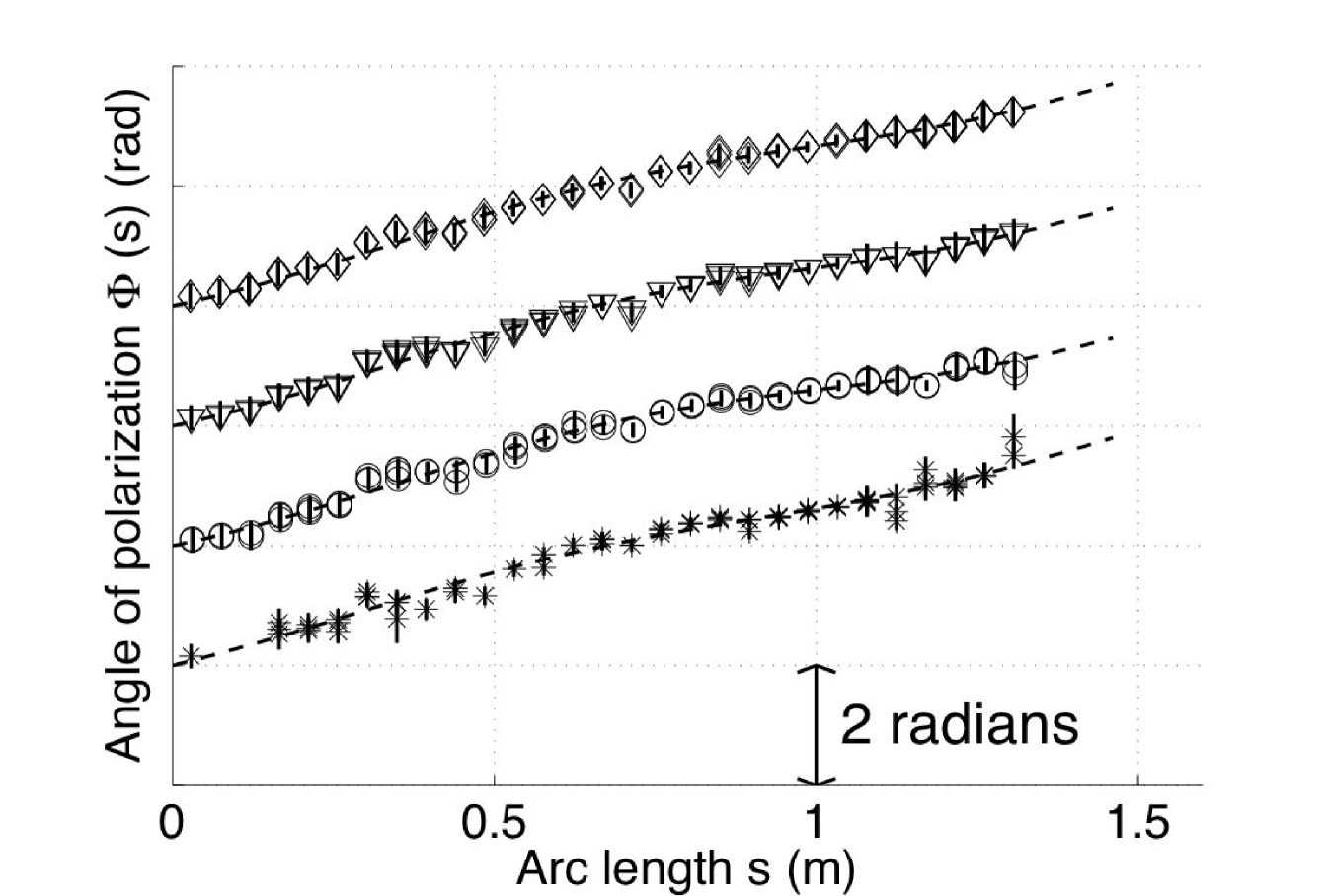
We obtain a linear coefficient for the signals filtered at four differents frequencies (bandwidth ). Numerical values are presented in Table 1.
| wavelength () | () | () | |||
|---|---|---|---|---|---|
| 2.53 | 0.31 | -0.03 | |||
| 2.35 | 0.45 | 0.03 | |||
| 2.45 | 0.39 | 0.05 | |||
| 2.50 | 0.38 | 0.07 |
5 Results and discussion
The theoretical Frénet torsion of the helix used in the experiment is . The fits performed from experimental data give an estimation of . We do not observe a significant dependency of with respect to the frequency or the velocity (see Table 1), which justifies the denomination “geometric phase” : the effect we observe is solely due to the geometry of the waveguide.
Apart from bending waves, compression waves and torsion waves can also propagate in the helix. In a straight rod, these propagation modes are not coupled and bending waves remain polarized at long times. In helices, the coupling between compression waves and torsion waves increases with curvature and torsion. Bending waves and torsional waves are therefore partially converted into each other, back and forth, during the propagation. This explains depolarization in our measurements and why we consider only the first oscillations of the signals.
We have filtered the polarized waves at four frequencies of the order of magnitude of the rate at which the propagation direction evolves . Such evolution rates imply that the regime is not adiabatic. Thanks to the dispersivity of the bending waves in the system, the adiabatic parameter can be varied by changing the filtering central frequency. Therefore filtering at several frequencies is equivalent to explore the non-adiabatic regime. No significant variations of the results are observable in the frequency range, which is an experimental evidence of the non-adiabaticity of the geometric phase, complementary to the theoretical derivation. Converted into lengths, this means that the wavelength of the bending wave is of the same order of magnitude as the length of a helix coil.
One may argue that the conversions between modes observed in the experiment are the classical equivalent of the transition between spin eigenstates of the quantum problem. By nature, however, these transitions are different. In the quantum problem, the transitions are of the first order in time but for the elastic waves, depolarization processes are of the second order, because an intermediate, unpolarized state is necessary. According to the dispersion relation in a helical waveguide [20], the intermediate state is mainly the torsional mode, and second the longitudinal compression mode.
6 Conclusion
We have demonstrated the existence of a geometric phase for elastic waves in a waveguide far from the adiabatic regime. We have investigated the results at several frequencies, or equivalently with several values of the adiabatic parameter, and observed no significant variations of the phase’s value. This is an experimental evidence, in addition to the theoretical derivation, that the observed phase is then not an adiabatic geometric phase with non-adiabatic corrections, but a non-adiabatic geometric phase for classical systems. Because there is no need to invoke the adiabatic approximation to preserve the polarization state, the geometric phase should extend to all frequencies in smooth waveguides with circular sections, a interesting result for waves with very large wavelengths. In quantum mechanics, the Aharonov-Anandan phase [4] shares the same non-adiabatic aspect as the non-quantum geometric phase studied in this letter.
In nature, polarized elastic waves, such as seismic S waves (shear waves) are observed under certain conditions, and the concept of geometric phase applies. The degree of polarization and the statistics of the polarization orientation in seismic signals created by a polarized source contain informations concerning the disorder of propagating medium that can be understood in terms of geometric phases.
7 Acknowledgments
The authors would like to thank É. Larose for discussions and B. de Cacqueray for his experimental help. This work was partially funded by the ANR-JC08-313906 SISDIF and CNRS/PEPS-PTI grants.
References
- [1] M. Born, E. Wolf, Principles of Optics, 7th Edition, Cambridge University Press, 2003.
- [2] M. V. Berry, Quantal phase factors accompanying adiabatic changes, Proc. R. Soc. Lond. A 392 (1984) 45–57.
- [3] J. H. Hannay, Angle variable holonomy in adiabatic excursion of an integrable Hamiltonian, J. Phys. A: Math. Gen. 18 (1985) 221–230.
- [4] Y. Aharonov, J. Anandan, Phase change during a cyclic quantum evolution, Phys. Rev. Lett. 58 (1987) 1593–1596.
- [5] J. Anandan, Geometric angles in quantum and classical physics, Phys. Lett. A 129 (1998) 201–207.
- [6] J. W. Zwanziger, M. Koenig, A. Pines, Berry’s phase, Annu. Rev. Phys. Chem. 41 (1990) 601–646.
- [7] A. Shapere, F. Wilczek, Geometric phases in physics, World Scientific, Singapour, 1990.
- [8] R. Bhandari, Polarization of light and topological phases, Physics Reports 281 (1997) 1–64.
- [9] A. Tomita, R. Y. Chiao, Observation of Berry’s topological phase by use of an optical fiber, Phys. Rev. Lett. 57 (1986) 937–940, 2471.
- [10] J. Segert, Photon Berry’s phase as a classical topological effect, Phys. Rev. A 36 (1987) 10–15.
- [11] J. Samuel, R. Bhandari, General setting for Berry’s phase, Phys. Rev. Lett. 60 (1988) 2339–2341.
- [12] J. von Bergmann, H. von Bergmann, Foucault pendulum through basic geometry, Am. J. Phys. 75 (2007) 888–892.
- [13] S. Pancharatnam, Generalized theory of interference and its applications i: coherent pencils, Proc. Ind. Acad. Sci. A 44 (1956) 247.
- [14] M. V. Berry, J. H. Hannay, Classical non-adiabatic angles, J. Phys. A: Math. Gen. 21 (1988) L325–L331.
- [15] M. V. Berry, M. A. Morgan, Geometric angle for rotated rotators, and the hannay angle of the world, Nonlinearity 9 (1996) 787–799.
- [16] P. K. Agarwal, H. Edelsbrunner, Y. Wang, Computing the writhing number of a polygonal knot, in: Proceedings of the 13th ACM-SIAM Symposium on Discrete Algorithms, ACM Press, New York, 2002, pp. 791–799.
- [17] V. Rossetto, A. C. Maggs, Writhing geometry of open DNA, J. Chem. Phys. 118 (2003) 9864–9874.
- [18] V. Rossetto, A. C. Maggs, Writhing geometry of stiff polymers and scattered light, Eur. Phys. J. B 118 (2002) 323–326.
- [19] M. Nakahara, Geometry, topology and physics, Graduate student series in physics, IOP publishing, Bristol, 2003.
- [20] F. Treyssède, Numerical investigation of elastic modes of propagation in helical waveguides, J. Acoust. Soc. Am. 121 (2007) 3398–3408.
- [21] J. Vidale, Complex polarization analysis of particle motion, Bull. of the Seismological Soc. of Am. 76 (5) (1986) 1393–1405.