Observation of Autler-Townes effect in a dispersively dressed Jaynes-Cummings system

The system studied in this experiment comprises a transmon [13], which can be thought of as a multi-level artificial ‘atom’ coupled to a single harmonic mode of a superconducting resonator. The coupled transmon-resonator system can be modelled to a good approximation [20] by a Jaynes-Cummings Hamiltonian [21] generalized to a multi-level atom [22, 23, 24]

Here $\omega_{r}$ is the bare resonator frequency, $a^{\dagger}\,$($a$) is the creation (annihilation) operator for the resonator mode, the transmon states $|j\rangle$ are labelled {${g,e,f,...}$}, and $g_{j,j+1}$ is the coupling strength of the $|j\rangle\leftrightarrow|j+1\rangle$ transition of the transmon with the resonator mode, assuming only coupling to quasi-resonance transitions. This Hamiltonian can be approximately diagonalized in the dispersive limit [11, 22, 25], $\Delta_{j,j+1}\equiv\omega_{j,j+1}-\omega_{r}\gg g_{j,j+1}$, where $\omega_{j,j+1}\equiv\omega_{j+1}-\omega_{j}$ is the frequency of the $|j\rangle\leftrightarrow|j+1\rangle$ transition. We can then write the diagonal Hamiltonian as a perturbative expansion in the small parameters $\lambda_{j,j+1}\equiv g_{j,j+1}/\Delta_{j,j+1}\ll 1$. In the context of our experiment, we truncate the transmon to a two level system with ground-state $|g\rangle$ and first-excited state $|e\rangle$. However, the finite anharmonicity of the transmon requires that we include perturbative shifts to the energy levels of the system due to the second-excited state $|f\rangle$ [20]. The dispersively diagonalized Hamiltonian up to second order in $\lambda_{j,j+1}$ is [11, 20]

where $\chi\simeq\chi_{ge}-\chi_{ef}/2$ is the effective dispersive shift of the resonator due to the transmon levels, $\chi_{j,j+1}\equiv g^{2}_{j,j+1}/\Delta_{j,j+1}$ are the partial couplings, $\widetilde{\omega}_{r}\simeq\omega_{r}-\chi_{ef}/2$ is the dressed resonator frequency, $\widetilde{\omega}_{ge}\simeq\omega_{ge}+\chi_{ge}$ is the dressed qubit transition frequency, and $\sigma_{z}$ is the z-Pauli spin operator for the qubit.

The last term in the Hamiltonian represents the dispersive shift of the resonator frequency by an amount $\pm\chi$ depending on the qubit state. It also produces an ac Stark shift of the qubit frequency by an amount $2\chi n$ due to $n=\langle n|a^{\dagger}a|n\rangle$ photons in the resonator [11]. In the strong dispersive limit the dispersive shift $\chi$ is much greater than the spectral line width of the qubit transition ($\Gamma$) or the resonator linewidth ($\kappa_{-}$). This enables us to resolve the Stark-shift of the qubit frequency due to each single photon in the resonator. The ac Stark-shift due to each constituent Fock state $|n\rangle$ results in a separate peak in the qubit spectrum. The stationary distribution $w_{n}$ of the Fock states, can then be well approximated by the relative areas under the individual photon-number peaks, with the average number of photons given by

For a finite temperature, and in the absence of resonator driving, $w_{n}$ is just the usual thermal distribution [16]. When the resonator is driven coherently from zero temperature [26], $w(n)$ approaches a Poisson distribution $w^{coh}_{n}=e^{-\bar{n}}(\bar{n})^{n}/n!$.

To simulate the system we use a density matrix formulation. We take into account Kerr-type nonlinearities by including terms up to fourth order in $\lambda_{j,j+1}$.

where $\zeta\approx(\chi_{ef}\lambda^{2}_{ef}-2\chi_{ge}\lambda^{2}_{ge}+7\chi_{ef}\lambda^{2}_{ge}/4-5\chi_{ge}\lambda^{2}_{ef}/4)$ is the resonator-qubit cross-Kerr coefficient and $\zeta^{\prime}\approx(\chi_{ge}-\chi_{ef})(\lambda^{2}_{ge}+\lambda^{2}_{ef})$ is the resonator self-Kerr coefficient [23, 24].

Dephasing and relaxation of the qubit and losses in the resonator are accounted for in the master equation in the Markovian approximation [20, 27]. For the resonator, we model the dissipation of photons as a decay rate $\kappa_{-}$. For the transmon, we model relaxation through a decay rate $\Gamma_{-}$ and pure dephasing through the dephasing rate $\gamma_{\phi}$ in the master equation. In our experiment, the finite population in the qubit excited state $|e\rangle$ and the resonator $n=1$ Fock state due to finite temperature are taken into account by including excitation rates $\kappa_{+}$ for the resonator and $\Gamma_{+}$ for the transmon, where $\kappa_{+}/\kappa_{-}=\Gamma_{+}/\Gamma_{-}\simeq\exp({-\hbar\omega_{r}/k_{B}T})$, giving us an estimate for the effective temperature of the system. The master equation for the density matrix ${\rho}$ can then be written as [20]

where the super-operator $\mathcal{D[{A}]{\rho}}\equiv{A\rho A^{\dagger}-(A^{\dagger}A\rho+\rho A^{\dagger}A})/2$ . We have neglected terms of the order $\lambda^{2}_{j,j+1}$ for each of the operators in the dissipation part of the master equation (8) after making the dispersive approximation.

The parameters $\chi,\Omega_{d},\Omega_{s},\zeta,\zeta^{\prime},\kappa_{-},\kappa_{+},\Gamma_{-},\Gamma_{+}$ and $\gamma_{\phi}$ are measured experimentally (section 3.3) and input into the simulation. We then solve (8) for the steady state solution $\dot{\rho}=0$. In our experiment, the qubit state-projective read-out signal is proportional to $\mbox{Tr}[\rho\sigma_{z}]$ in the steady state.

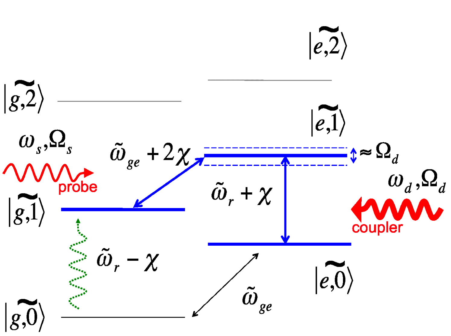
When the transition between two quantum levels is driven strongly with a resonant drive field, the resulting ‘dressed’ system can be equivalently viewed as two split levels, with splitting equal to the Rabi frequency of the drive field (figure 1). This splitting can be observed spectroscopically by probing transitions to a third level in the system, which comprises the Autler-Townes effect [17]. In this section, we take a closer look at (7) to understand the mechanism of the Autler-Townes splitting of the $n=1$ photon peak observed in our experiment. The Kerr-type nonlinearities are neglected in the context of this simple model.

We begin by truncating the set of basis states to the four lowest dressed levels $|\widetilde{g,0}\rangle$, $|\widetilde{e,0}\rangle$, $|\widetilde{g,1}\rangle$ and $|\widetilde{e,1}\rangle$ (figure 1). In the experiment, the $|\widetilde{e,0}\rangle\leftrightarrow|\widetilde{e,1}\rangle$ transition is driven by a strong ‘coupler’ field with strength $\Omega_{d}$ and detuning $(\widetilde{\omega}_{r}+\chi)-\omega_{d}\equiv\widetilde{\Delta}_{d}+\chi$, and the $|\widetilde{g,1}\rangle\leftrightarrow|\widetilde{e,1}\rangle$ is ‘probed’ by a weak field of strength $\Omega_{s}$ and detuning $(\widetilde{\omega}_{ge}+2\chi)-\omega_{s}\equiv\widetilde{\Delta}_{s}+2\chi$ (figure 1).

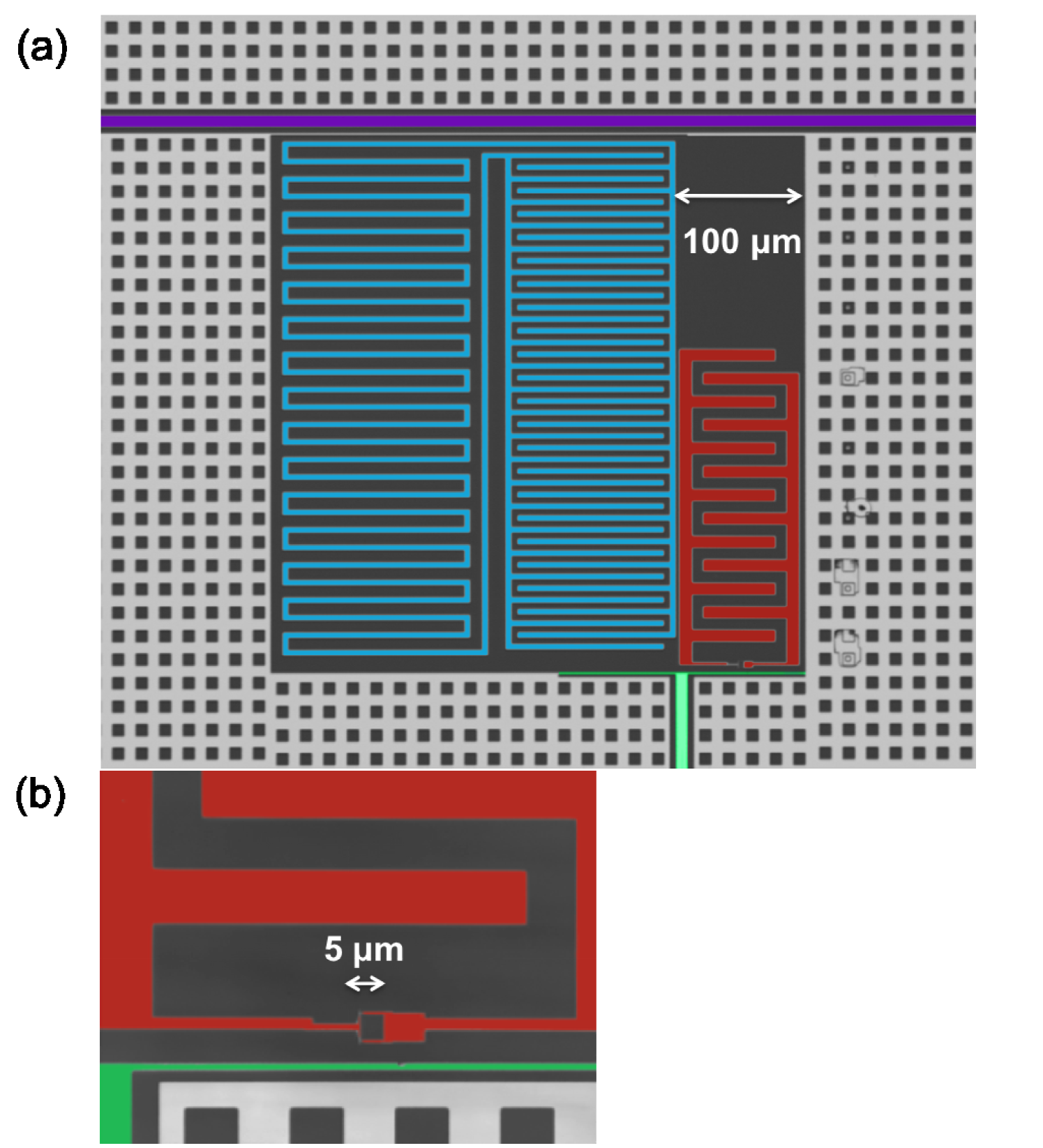
Figure 2 shows the transmon [13] coupled to a superconducting lumped-element resonator [28], which is in turn coupled to a coplanar waveguide transmission line used for excitation and measurement. The transmon is formed from two Josephson junctions (junction area $\approx 100\times 100\$ nm²) shunted by an interdigitated capacitor with finger widths of 10 $\mu$m, lengths of 70 $\mu$m, and separation between fingers of 10 $\mu$m. The junctions are connected to form a superconducting loop with a nominal loop area of $4\times 4.5\,\mu$m². The Josephson junction loop is placed close to a shorted current bias line to finely tune the critical current of the parallel junctions and hence the transition frequency of the qubit.

The device was fabricated by depositing a $100\,$nm thin film of aluminium by thermal evaporation on a commercial c-plane sapphire substrate. The resonator, transmission line, and on-chip flux bias line were patterned using photolithography and etched with a standard aluminium etchant. The transmon was subsequently patterned using electron-beam lithography and the Al/AlO_x/Al tunnel junctions were formed by double-angle evaporation with an intermediate oxygen exposure step.

The device was mounted in a hermetically sealed copper box and attached to the mixing chamber of an Oxford Kelvinox 100 dilution refrigerator with a base temperature of $20\,$ mK. To isolate the device from thermal noise at higher temperatures, the input microwave line to the device has a 10 dB attenuator mounted at 4 K, 20 dB at 0.7 K, and 30 dB at 20 mK on the mixing chamber. On the output (i.e. read-out) microwave line, two 18 dB isolators with bandwidths from 4 to 8 GHz are placed in series at 20 mK. The output microwave signal then goes through a 3 dB attenuator and a high electron mobility transistor amplifier at 4 K before being amplified further at room temperature and mixed down to an intermediate frequency (IF) of 10 MHz.

Three microwave sources are used in the measurement: probe, coupler, and read-out. The read-out and probe tones are pulsed on and off, while the coupler tone is applied continuously for the duration of the measurement. To measure the excited-state population of the transmon, a high power (i.e. 50 dB larger than the power of the coupler tone) at a frequency corresponding to the bare cavity is applied [29]. This read-out relies on the Jaynes-Cummings nonlinearity of the coupled resonator-qubit system [24, 30] and depending on the state of the system, either a large transmissivity is observed (e.g. $|g\rangle$ state) or small transmissivity (e.g. $|e\rangle$ state).

For spectroscopic measurements, a probe pulse is first applied for a duration of $5\,\mu$s at an amplitude just large enough to saturate the qubit transition without causing large power broadening. A read-out pulse of duration $5\,\mu$s is applied $20\,$ns after turning off the probe. The mixed down IF signal is digitized using a data acquisition card and the in-phase and quadrature components are demodulated before being recorded.

From spectroscopic and time-domain measurements the main system parameters were determined. The resonator has a bare resonant frequency $\omega_{r}/2\pi=5.464\,$GHz, internal quality factor $Q_{I}=190,000$, and a loaded quality factor $Q_{L}\equiv\omega_{r}/\kappa_{-}=18,000$. The parallel resistance of the Josephson junctions yielded a maximum Josephson energy $E_{J,max}/h\approx 25\,$GHz and the transmon has a Coulomb charging energy of $E_{c}/h=250\,$MHz. This gives a maximum ground-to-first excited state transition frequency, $\omega_{ge,max}/2\pi\simeq(\sqrt{8E_{J,max}E_{c}}-E_{c})/h=7.1\,$GHz for the qubit. The qubit transition frequency was tuned using a combination of an external superconducting magnet and the on-chip flux bias to $\widetilde{\omega}_{ge}/2\pi=4.982\,$GHz, which corresponds to a detuning of $\Delta_{ge}/2\pi=482\,$ MHz from the resonator. From spectroscopic measurements, we determined the effective dispersive shift $\chi/2\pi=4.65\,$MHz, and the parameters $\chi_{ge}/2\pi=-10\,$ MHz and $\chi_{ef}/2\pi=-10.7\,$MHz. From the definitions of $\chi_{ge}$ and $\chi_{ef}$, we determine $g_{ge}/2\pi=70\,$MHz and $g_{ef}/2\pi=89\,$ MHz. The resonator self-Kerr coefficient $\zeta^{\prime}/2\pi=85\,$kHz and the transmon-resonator cross-Kerr coefficient $\zeta/2\pi=23\,$kHz are then determined from (5).

Time-domain coherence measurements performed at this resonator-qubit ($\Delta_{ge}/2\pi=482\,$ MHz) detuning revealed a qubit relaxation time $T_{1}=1/(\Gamma_{-}+\Gamma_{+})=1.6\,\mu$s^-1 and a Rabi decay time $T^{\prime}=1.6\,\mu$s for the first excited state of the qubit. From these measurements, the pure dephasing rate is estimated at $\gamma_{\phi}\equiv 1/T_{\phi}\approx 2\times 10^{5}\,$s^-1.

Figure 3(a) shows spectroscopy of the transmon with no drive field applied to the resonator. The spectrum shows the dressed qubit ground-to-first excited state transition at $\widetilde{\omega}_{ge}/2\pi=4.982\,$GHz. The smaller spectroscopic peak detuned by -9.3 MHz at $(\widetilde{\omega}_{ge}-2\chi)/2\pi=4.973\,$GHz is due to one $\widetilde{\omega}_{r}-\chi/2\pi=5.474\$GHz photon occasionally being present in the resonator [16] from thermal excitations. From the relative areas under the two spectral peaks, we estimate a fractional thermal population of $n_{th}=0.1$ photons, corresponding to a temperature of about $120\,$mK for the resonator. This effective temperature is much higher than the base temperature $\sim 20\,$mK of the dilution refrigerator, possibly due to a leakage of higher frequency photons [7, 8].

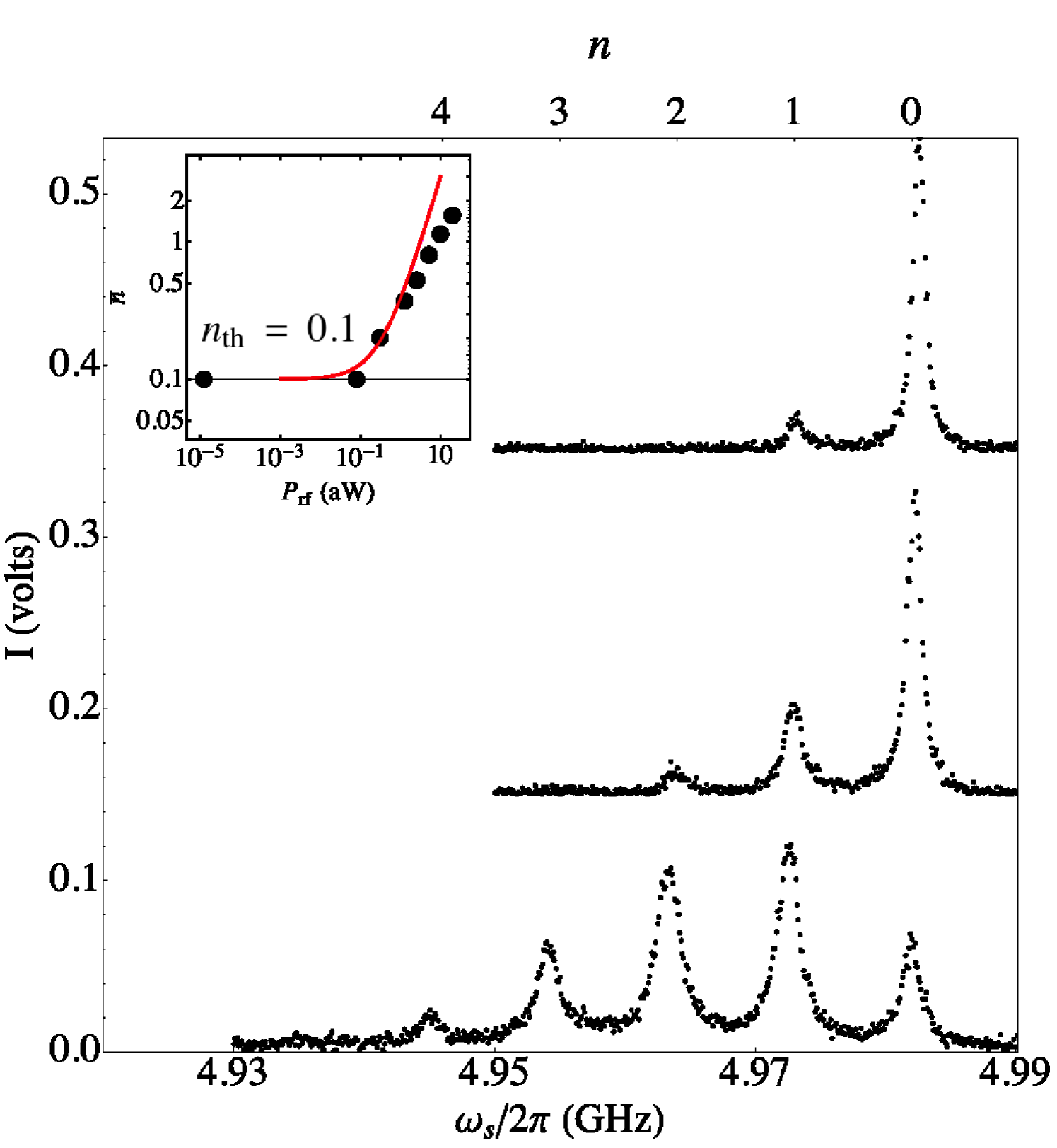
Upon driving the resonator with a coupler tone at $\omega_{d}/2\pi=5.474\,$GHz, which is resonant with the transition $|\widetilde{g,0}\rangle\leftrightarrow|\widetilde{g,1}\rangle$ (figure 1), we increase the mean occupancy of the resonator from its equilibrium value and create a coherent state. Since the coherent state is a superposition of Fock states, the qubit spectrum has multiple peaks, one for each Fock state. When applying a power of $P_{rf}=1.25\,$aW at the dressed resonator frequency (figure 3(b)), an increase in the height of the $\widetilde{\omega}_{ge}-2\chi$ peak is observed and a spectral peak at $\widetilde{\omega}_{ge}-4\chi$ begins to appear. The peak at $\widetilde{\omega}_{ge}$ is still the largest. Figure 3(c) shows the spectrum for an applied resonator drive power of 25 aW. In this case, more spectral peaks are observed and the $\widetilde{\omega}_{ge}-2\chi$ is the largest.

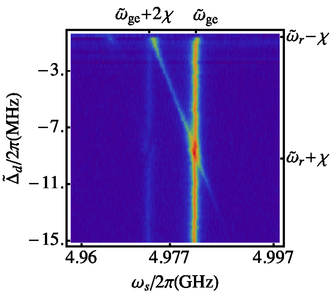
Figure 4 shows two-tone spectroscopy of the qubit as we vary the frequency of the coupler tone. In this plot, the vertical bands at frequencies $\omega_{s}/2\pi=4.982\,$GHz and 4.973 GHz are just the $n=0$ and $n=1$ photon peaks as shown in figure 3. The prominent diagonal band seen between the $n=0$ and $n=1$ photon bands in this figure corresponds to a two-photon ‘blue’ sideband transition from the $|\widetilde{g,0}\rangle$ to $|\widetilde{e,1}\rangle$ [31]; the sum of the frequencies ($\omega_{s},\omega_{d}$) of the drive photons along this diagonal band is equal to the corresponding transition frequency. In general, a diagonal band with slope $-1/n$ should appear when the detunings of the drives satisfy $\widetilde{\Delta}_{s}-n\widetilde{\Delta}_{d}=n\chi$ corresponding to the sideband transition $|g,n-1\rangle\leftrightarrow|e,n\rangle$. For example, the sideband transition $|\widetilde{g,0}\rangle\leftrightarrow|\widetilde{e,1}\rangle$ level appears as a band of slope $-1$ and the $|\widetilde{g,1}\rangle\leftrightarrow|\widetilde{e,2}\rangle$ transition appears as a faintly visible band of slope $-1/2$ in figure 4.

Another feature of the data in figure 4 is a small splitting in the thermal $n=1$ photon peak when the frequencies of the probe and coupler tones are ($\omega_{s},\omega_{d})\simeq(\widetilde{\omega}_{ge}+2\chi,\widetilde{\omega}_{r}+\chi$). We examine this splitting more closely in this section. Here we follow the convention of section 2.3 and refer to the strengths of the probe and coupler tones in terms their Rabi frequencies $\Omega_{s}$ and $\Omega_{d}$. The Rabi frequency of the coupler tone $\Omega_{d}$ can be independently calibrated from the power of the coupler tone using the relation

while the Rabi frequency $\Omega_{s}$ of the probe tone was measured independently from the Rabi oscillations of the qubit.

Figure 5(a)-(c) shows measurements of the splitting in the thermal $n=1$ photon peak as we vary the strength of the coupler tone while keeping the strength of the probe tone fixed $\Omega_{s}/2\pi\simeq 0.3\,$MHz. Figure 5(a) shows that when we apply a coupler tone with strength $\Omega_{d}/2\pi\simeq 1.3\,$MHz, we observe a splitting in the thermal $n=1$ photon peak with a splitting size that is almost equal to $\Omega_{d}$. In figure 5(b), we lower the strength of the coupler to $\Omega_{d}/2\pi\simeq 1\,$MHz and we notice a corresponding decrease in the splitting size to $\sim 1\,$MHz. Upon further lowering the strength of the coupler to $\Omega_{d}/2\pi\simeq 0.6\,$MHz, the splitting decreases in size to $\sim 0.6\,$MHz.

The splitting size can be understood based on an Autler-Townes mechanism (section 2.3) shown in figure 1. To begin with, the $|\widetilde{g,1}\rangle$ level is populated due to thermal excitation of photons in the resonator [7, 8]. Subsequently the probe and coupler tones are applied on resonance with the transitions $|\widetilde{g,1}\rangle\leftrightarrow|\widetilde{e,1}\rangle$ and $|\widetilde{e,0}\rangle\leftrightarrow|\widetilde{e,1}\rangle$ (see section 2.3) respectively. In the presence of the two drive fields, the $|\widetilde{e,1}\rangle$ level splits into a pair of levels separated by $\delta=(\Omega^{2}_{s}+\Omega^{2}_{d})^{1/2}$ (10). In the limit $\Omega_{d}\gg\Omega_{s}$ this splitting is almost equal to $\Omega_{d}$ and is observed spectroscopically upon probing the $|\widetilde{g,1}\rangle\leftrightarrow|\widetilde{e,1}\rangle$ transition.

The simple model in (9) also predicts the overall ‘shape’ of the splitting in the $(\omega_{s},\omega_{d})$ plane in figure 5(a)-(c). When $\tilde{\Delta}_{s}+2\chi=0$ and $\tilde{\Delta}_{d}+\chi\neq 0$, only the $|\widetilde{g,1}\rangle\leftrightarrow|\widetilde{e,1}\rangle$ transition is resonantly driven, while the influence of level $|\widetilde{e,0}\rangle$ is energy suppressed. This explains the vertical band corresponding to the $n=1$ photon peak at $4.973\,$GHz. When $\tilde{\Delta}_{s}+2\chi=\tilde{\Delta}_{d}+\chi\neq 0$, the difference of the drive frequencies corresponds to the $|\widetilde{e,0}\rangle\leftrightarrow|\widetilde{g,1}\rangle$ transition. This two-photon ‘red’ sideband transition [31] explains the slope $+1$ of the splitting in the figure 5.

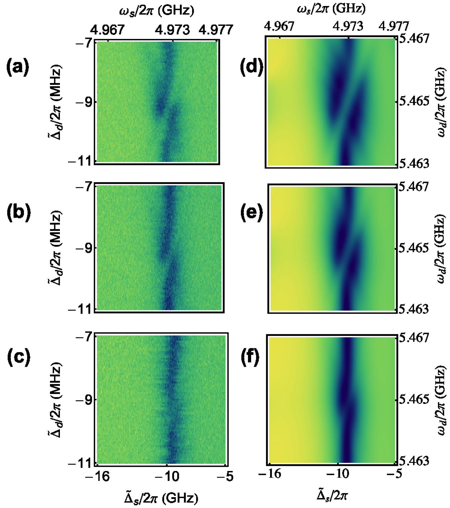
Figure 5(d)-(f) shows simulations of the system-bath master equation at the steady state (section 2.2) in the region around the thermal $n=1$ photon peak when driving the coupler with a strength of $\Omega_{d}/2\pi$ = 1.3 MHz (d), 1 MHz (d), and 0.6 MHz (f). The parameters $\chi,\Omega_{d},\Omega_{s},\zeta,\zeta^{\prime},\kappa_{-},\kappa_{+},\Gamma_{-},\Gamma_{+}$ and $\gamma_{\phi}$ in the master equation were determined from independent experiments (section 3.3) and equation (8) was then solved for $\rho$ for the steady state solution. Here we plot $\mathrm{Tr(\rho.\sigma_{z})}$ to simulate the qubit state-projective read-out in our experiment [24, 29, 30]. We included the two lowest qubit levels $|g\rangle,|e\rangle$, the ten lowest resonator levels, the resonator self-Kerr and qubit-resonator cross-Kerr terms in the simulation. The population in the $n=1$ Fock state of the resonator and the $|e\rangle$ state of the transmon due to finite temperature were taken into account through the excitation rates $\kappa_{+}\approx\kappa_{-}/10$, $\Gamma_{+}\approx\Gamma_{-}/10$ in the system master equation (8).

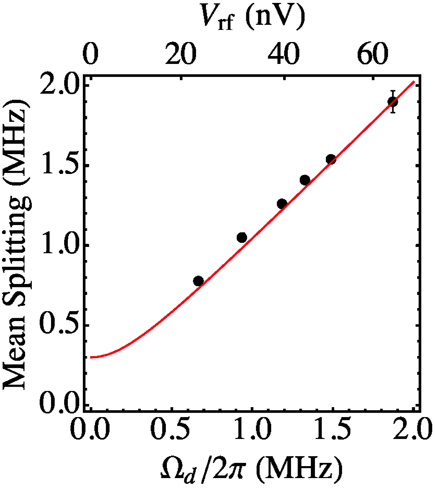
Finally, figure 6 shows the experimentally measured splitting vs the Rabi frequency of the coupler. The Rabi frequency of the coupler $\Omega_{d}$ was calibrated independently from the power of the coupler drive using (12). The root-mean-square voltage $V_{rf}\propto(P_{rf})^{1/2}$ of the coupler at the device is calculated from $P_{rf}$ assuming a 50$\,\Omega$ impedance for the transmission line. The red curve in the figure 6 is the splitting size $\delta/2\pi\simeq(\Omega^{2}_{d}+\Omega^{2}_{s})^{1/2}/2\pi$ predicted by the simple model (10) for a fixed $\Omega_{s}/2\pi\simeq 0.3\,$MHz and it agrees well with the experimental data. Here we see that the observed Autler-Townes splitting is nearly linear in the amplitude of the coupler drive voltage $V_{rf}$ and is almost equal to the Rabi frequency of the coupler field, as expected from (10).

References

- [1] Clarke John and Wilhelm Frank K. Nature, 453(7198):1031–42, 2008.
- [2] Devoret M H and Martinis J M. Quantum Information Processing, 3(October):163–203, 2004.
- [3] Chang J, Vissers M R, Corcoles A D, Sandberg M, Gao J, Abraham D W, Chow J M, Gambetta J M, Rothwell M B, Keefe G A, Steffen M, and Pappas D P. arXiv preprint arXiv:1303.4071, pages 3–6, 2013.
- [4] Manucharyan Vladimir E, Koch Jens, Glazman Leonid I, and Devoret Michel H. Science, 326(5949):113–6, 2009.
- [5] Paik Hanhee, Schuster D I, Bishop Lev S, Kirchmair G, Catelani G, Sears A P, Johnson B R, Reagor M J, Frunzio L, Glazman L I, Girvin S M, Devoret M H, and Schoelkopf R J. Phys. Rev. Lett., 107(24):240501, 2011.
- [6] Barends R, Kelly J, Megrant A, Sank D, Jeffrey E, Chen Y, Yin Y, Chiaro B, Mutus J, Neill C, O’Malley P, Roushan P, Wenner J, White T C, Cleland A N, and J M Martinis. arXiv preprint arXiv:1304.2322, (c):10, 2013.
- [7] Córcoles Antonio D, Chow Jerry M, Gambetta Jay M, Rigetti Chad, Rozen J R, Keefe George A, Beth Rothwell Mary, Ketchen Mark B, and Steffen M. App. Phys. Lett., 99(18):181906, 2011.
- [8] Wenner J, Yin Yi, Lucero Erik, Barends R, Chen Yu, Chiaro B, Kelly J, Lenander M, Mariantoni Matteo, Megrant A, Neill C, O’Malley P J J, Sank D, Vainsencher A, Wang H, White T C, Cleland A N, and Martinis J M. Phys. Rev. Lett., 110(15):150502, 2013.
- [9] Hood C J, Lynn T W, Doherty A C, Parkins A S, and Kimble H J. Science, 287(5457):1447–1453, 2000.
- [10] Raimond J M, Brune M, and Haroche S. Rev. Mod. Phys., 73(3):565–582, 2001.
- [11] Blais Alexandre, Huang Ren-Shou, Wallraff Andreas, Girvin S M, and R J Schoelkopf. Phys. Rev. A, 69(6):062320, 2004.
- [12] Wallraff A, Schuster D I, Blais A, Frunzio L, Huang R-S, Majer J, Kumar S, Girvin S M, and Schoelkopf R J. Nature, 431(7005):162–7, 2004.
- [13] Koch Jens, Yu Terri M, Gambetta Jay, Houck A A, Schuster D I, Majer J, Blais Alexandre, Devoret M H, Girvin S M, and Schoelkopf R J. Phys. Rev. A, 76(4):42319, 2007.
- [14] Schuster D I, Houck A A, Schreier J A, Wallraff A, Gambetta J M, Blais A, Frunzio L, Majer J, Johnson B, Devoret M H, Girvin S M, and Schoelkopf R J. Nature, 445(7127):515–8, 2007.
- [15] You J Q and Nori Franco. Nature, 474(7353):589–97, 2011.
- [16] Dykman M I and Krivoglaz M A. Fiz. Tverd. Tela, 29(2):368–376, 1987.
- [17] Autler S H and Townes C H. Phys. Rev., 100(2):703–722, 1955.
- [18] Baur M, Filipp S, Bianchetti R, Fink J, Göppl M, Steffen L, Leek P, Blais A, and Wallraff A. Phys. Rev. Lett., 102(24):243602, 2009.
- [19] Sillanpää Mika, Li Jian, Cicak Katarina, Altomare Fabio, Jae Park, Raymond Simmonds, G Paraoanu, and Pertti Hakonen. Phys. Rev. Lett., 103(19):193601, 2009.
- [20] Bishop Lev S. Circuit Quantum Electrodynamics. PhD thesis, Yale University, 2010.
- [21] Jaynes E T and Cummings F W. Proc. IEEE, 51(1):89–109, 1963.
- [22] Boissonneault Maxime, Gambetta J M, and Blais Alexandre. Phys. Rev. A, 79(1):013819, 2009.
- [23] Gambetta Jay, Blais Alexandre, Schuster D I, Wallraff A, Frunzio L, Majer J, Devoret M H, Girvin S M, and Schoelkopf R J. Phys. Rev. A, 74(4):042318, 2006.
- [24] Boissonneault Maxime, Gambetta J M, and Blais Alexandre. Phys. Rev. Lett., 105(10):100504, 2010.
- [25] Carbonaro P, Compagno G, and Persico F. Phys. Lett. A, 73(2):97–99, 1979.
- [26] Glauber Roy J. Phys. Rev., 131(6):2766–2788, 1963.
- [27] Lindblad G. Commun. math. Phys, 48:119–130, 1976.
- [28] Kim Z, Suri B, Zaretskey V, Novikov S, Osborn K D, Mizel A, Wellstood F C, and Palmer B S. Phys. Rev. Lett., 106(12):120501, 2011.
- [29] Reed M D, DiCarlo L, Johnson B R, Sun L, Schuster D I, Frunzio L, and Schoelkopf R J. Phys. Rev. Lett., 105(17):173601, 2010.
- [30] Bishop Lev S, Ginossar Eran, and Girvin S M. Phys. Rev. Lett., 105(10):100505, 2010.
- [31] Wallraff A, Schuster D I, Blais A, Gambetta J M, Schreier J, Frunzio L, Devoret M H, Girvin S M, and Schoelkopf R J. Phys. Rev. Lett., 99(5):50501, 2007.
- [32] Boller K J, Imamoğlu A, and Harris S E. Phys. Rev. Lett., 66(20):2593–2596, 1991.
- [33] Ian Hou, Liu Yu-xi, and Nori Franco. Phys. Rev. A, 81(6):063823, 2010.
- [34] Hau L V, Harris S E, Dutton Zachary, and Behroozi Cyrus H. Nature, 397(February):594–598, 1999.
- [35] Murali K V R M, Dutton Z, Oliver W D, Crankshaw D S, and Orlando T P. Phys. Rev. Lett., 93(8):087003, 2004.
- [36] Abdumalikov A A, Astafiev O, Zagoskin A M, Pashkin Yu A, Nakamura Y, and Tsai J S. Phys. Rev. Lett, 104(19):193601, 2010.