IceCube Collaboration
Observation of the cosmic-ray shadow of the Moon with IceCube
Abstract
We report on the observation of a significant deficit of cosmic rays from the direction of the Moon with the IceCube detector. The study of this “Moon shadow” is used to characterize the angular resolution and absolute pointing capabilities of the detector. The detection is based on data taken in two periods before the completion of the detector: between April 2008 and May 2009, when IceCube operated in a partial configuration with 40 detector strings deployed in the South Pole ice, and between May 2009 and May 2010 when the detector operated with 59 strings. Using two independent analysis methods, the Moon shadow has been observed to high significance () in both detector configurations. The observed location of the shadow center is within of its expected position when geomagnetic deflection effects are taken into account. This measurement validates the directional reconstruction capabilities of IceCube.
pacs:
96.50.S-,95.85.Ry,96.20.-n,91.25.-r,29.40.KaI Introduction
IceCube is a km3-scale Cherenkov detector deployed in the glacial ice at the geographic South Pole. Its primary goal is to search for astrophysical sources of high-energy neutrinos. A major background for this search is the high rate of atmospheric muons produced when cosmic rays with energies above a few TeV interact with the Earth’s atmosphere. The rate of muon events in IceCube above several hundred GeV dominates the total trigger rate of the detector, and is approximately six orders of magnitude higher than the rate of neutrino-induced events.
The incoming direction of multi-TeV cosmic muons is on average within 0.1∘ of arrival direction of the primary cosmic-ray particle Abbasi et al. (2013). This implies that the distribution of incoming muons should mimic the almost isotropic distribution of TeV cosmic rays in the sky Abbasi et al. (2010a, 2011a). An important feature of the angular distribution of cosmic rays is the presence of a relative deficit in the flux of cosmic rays coming from the direction of the Moon. This effect, due to the absorption of cosmic rays by the Moon, was first predicted by Clark in 1957 Clark (1957), and its observation has been used by several experiments as a way of calibrating the angular resolution and the pointing accuracy of their particle detectors (see Ambrosio et al. (2003), Achard et al. (2005), Oshima et al. (2010), Adamson et al. (2011), or Bartoli et al. (2011) for recent results.)
For IceCube, the Moon shadow analysis is a vital and unique verification tool for the track reconstruction algorithms that are used in the search for point-like sources of astrophysical neutrinos Abbasi et al. (2011b), among other analyses. In this paper we will report on the observation of the Moon shadow using data taken between April 2008 and May 2010, before the completion of the IceCube Neutrino Observatory in December 2010.
Two independent analysis methods were used in the search for the Moon shadow. The first analysis performs a binned, one-dimensional search for the Moon shadow that compares the number of events detected from the direction of the Moon to the number of background events recorded at the same declination as the Moon but at a different right ascension. The second method uses an unbinned, two-dimensional maximum likelihood algorithm that retrieves the best fit value for the total number of events shadowed by the Moon.
Both methods show consistent results, and constitute the first statistically significant detection of the shadow of the Moon using a high-energy neutrino telescope.
II Detector Configuration and Data sample
II.1 The IceCube detector
The IceCube neutrino telescope uses the deep Antarctic ice as a detection medium. High-energy neutrinos that interact with nucleons in the ice produce relativistic leptons that emit Cherenkov radiation as they propagate through the detector volume. This Cherenkov light is detected by a volumetric array of 5160 Digital Optical Modules (DOMs) deployed at depths between 1450 m and 2450 m below the ice surface. Each DOM consists of a 25 cm diameter photomultiplier tube (PMT) Abbasi et al. (2010b) and the electronics for signal digitization Abbasi et al. (2009) housed inside a pressure-resistant glass sphere.
The DOMs are attached to 86 strings that provide mechanical support, electrical power, and a data connection to the surface. Consecutive DOMs in each string are vertically separated by a distance of about 17 m, while the horizontal spacing between strings is about 125 m. A compact group of eight strings with a smaller spacing between DOMs is located at the bottom of the detector and forms DeepCore Abbasi et al. (2012), which is designed to extend the energy reach of IceCube to lower neutrino energies. The IceTop surface array, devoted to the detection of extensive air showers from cosmic rays with energies between 300 TeV and 1 EeV, completes the instrumentation of the observatory.
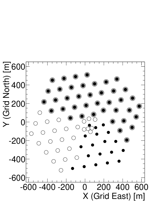
The construction of IceCube began in 2005 and was completed in December 2010. During construction, the detector operated in several partial configurations. Data from two different configurations were used in this paper: between 2008 and 2009 the detector operated with 40 strings deployed in the ice (IC40), and between 2009 and 2010 the detector operated in its 59-string configuration (IC59). The layout of the two detector configurations used in this work can be seen in Fig. 1.
II.2 Data sample
In order to reduce the rate of noise-induced events, IceCube DOMs are operated in a coincidence mode called Hard Local Coincidence (HLC). During the operation of IC40 and IC59 the HLC requirement was met if photon hits were detected within a s window in two nearest neighbor or next-to-nearest neighbor DOMs. The detection of HLC hits leads to a full readout and transmission to the surface of the digitized PMT signals. A trigger condition is then used to combine these photon hits into a candidate event. The main trigger in IceCube is a simple multiplicity trigger called SMT8 that requires HLC hits in eight DOMs within 5 s. For each trigger, all HLC hits within a s window are recorded and merged into a single event.
The majority of events detected by IceCube are due to down-going muons produced in the interaction of high energy cosmic rays with the Earth’s atmosphere. During the operation of IC40, the cosmic muon-induced trigger rate was about 1.1 kHz, which increased to about 1.7 kHz during the IC59 data-taking period. This high rate of cosmic-ray muon events provides a high-statistics data set that can be used to search for the Moon shadow.
Since the rate of data transfer from the South Pole via the South Pole Archival and Data Exchange (SPADE) satellite communication system is limited to about 100 Gb per day, only a limited number of muon events can be transmitted to North over the satellite. For this reason, the data used in this analysis were taken using a dedicated online filter that selects only events passing minimum quality cuts and reconstructed within a predefined angular acceptance window around the Moon.
A fast likelihood-based muon track reconstruction Ahrens et al. (2004) is performed at the South Pole to obtain the arrival direction of each event. The reconstructed direction of the muon track is then compared to the position of the Moon in the sky, which is calculated using the publicly-available SLALIB library of astronomical routines Wallace (1994).
An event satisfies the Moon filter selection criterium if at least 12 DOMs in 3 different strings record photon hits, and if the reconstructed direction is within 10∘ of the Moon position in declination and 40 in right ascension (where is the declination of the event and the cosine factor accounts for projection effects.)
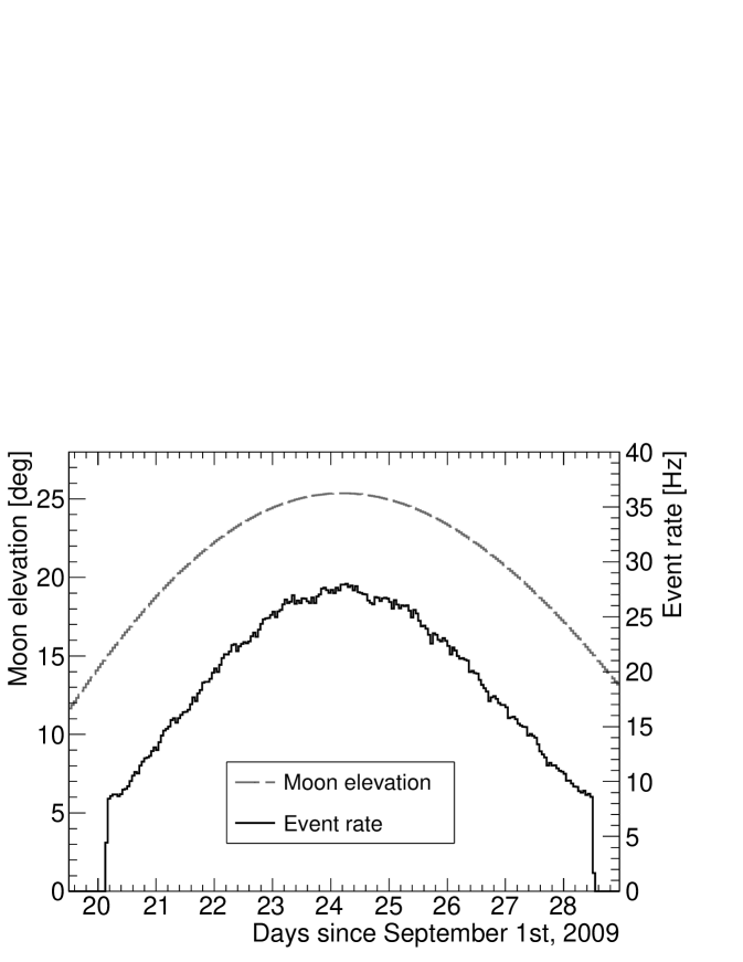
The filter is enabled when the Moon is at least above the horizon. Due to the particular geographic location of IceCube at the South Pole, the Moon rises above this threshold only once per month, as its elevation above the horizon changes slowly over the course of days. Since the number of muon events recorded by IceCube is a strong function of the elevation angle, the rate of events that pass the acceptance window condition changes during this period as this window follows the apparent motion of the Moon at the South Pole. The strong correlation between Moon elevation and rate of events passing the Moon filter is shown in Fig. 2. The maximum event rate is also modulated over a longer time scale of 18.6 years (known as the lunar draconic period Meyers and Shore (1989)) in which the maximum elevation of the Moon above the horizon at the South Pole oscillates between the extreme values of and . The maximum Moon elevation during the IC40 data-taking period was , while for IC59 was . Approximately muon events passing the Moon filter condition were recorded during the IC40 data-taking period, and about events were recorded during the operation of the IC59 configuration.
Once these events have been transferred from the South Pole, an iterative maximum-likelihood reconstruction algorithm is applied to the data set to obtain a more precise track direction Ahrens et al. (2004). The algorithm also determines the angular uncertainty in the reconstructed track direction by mapping the likelihood space around the best track solution and fitting it with a paraboloid function Neunhöffer (2006). A narrow paraboloid indicates a precise reconstruction, while a wide paraboloid indicates a larger uncertainty in the reconstructed direction of the muon track. The contour line of the paraboloid function defines an error ellipse for the reconstructed direction of the track. In this analysis, a single, one dimensional estimator of the uncertainty is obtained by calculating the RMS value of the semi-major axes of that error ellipse.
The likelihood-based track reconstruction algorithm used in this work is based on the leading-edge times of the first light pulses recorded by each DOM. For the fast track reconstruction at the South Pole the single-photo-electron (SPE) fit is used. In this fit, the likelihood that the first photon arrived at the pulse leading-edge times is maximized. The photons arriving at later times are ignored.
Neutrino point source searches rely on the multi-photo-electron (MPE) fit. In the MPE fit, the total number of photo-electrons in each DOM is taken into account by multiplying the likelihood that a photon was detected at the first leading edge time with the probability that the remaining photons arrived later Ahrens et al. (2004). For bright, i.e. high-energy, events in simulated data the MPE fit results in a slightly better angular resolution than the SPE fit. Also the number of direct (unscattered) photons associated with the reconstructed track tends to be larger with the MPE fit than with the SPE fit. This makes this quantity as well as related quantities more effective for selecting well-reconstructed events. The MPE fit is discussed further in Section V.2.2.
The track reconstruction algorithms use the local detector coordinate system and the direction of a reconstructed track is given as a zenith and azimuth angle. Using the event times as recorded by the data acquisition system these are transformed into a right ascension and declination , which are the more natural variables for searches of neutrino point-like sources.
III Simulation
III.1 Cosmic ray energy and composition
The muons produced in the interaction between the cosmic rays and the atmosphere must traverse several kilometers of ice before reaching the IceCube detector, losing energy in the process. This sets a lower limit of several hundred GeV on the energy of the muons at ground level that would trigger the detector. By extension, the primary cosmic-ray particle needed to produce this kind of muon should have an energy of at least several TeV. In the following, we will refer to the energy of the primary cosmic ray, not the muons, unless specified otherwise.
Given that this analysis deals with cosmic-ray showers near the energy threshold of the detector, the number of muons produced in each shower that reach the detector is small. Most events in the Moon data sample are composed of one or two energetic muons, and only 2% of the events have muon multiplicities higher than ten.
The detailed energy scale for the IC40 and IC59 data sets was determined using simulated cosmic ray air showers created with the CORSIKA Monte Carlo code Heck et al. (1998) using the SIBYLL model of high-energy hadronic interactions Ahn et al. (2009). The chemical composition and spectral shape of the cosmic rays generated in this simulation follow the polygonato model Hörandel (2003).
From these simulations, we estimate that the median energy of the primary cosmic rays that trigger the IceCube detector is 20 TeV, while the median energy of events that satisfy the Moon filter condition is about 40 TeV for both IC40 and IC59, with 68% of the events between 10 TeV and 200 TeV. The increased median energy of the filtered sample is due to the greater average zenith angles of the cosmic rays that pass the filter, which requires primary particles with enough energy to produce muons able to traverse more ice and trigger IceCube. The muons produced by cosmic rays passing the Moon filter have a mean energy of about 2 TeV at ground level and reach the detector with a mean energy of 200 GeV.
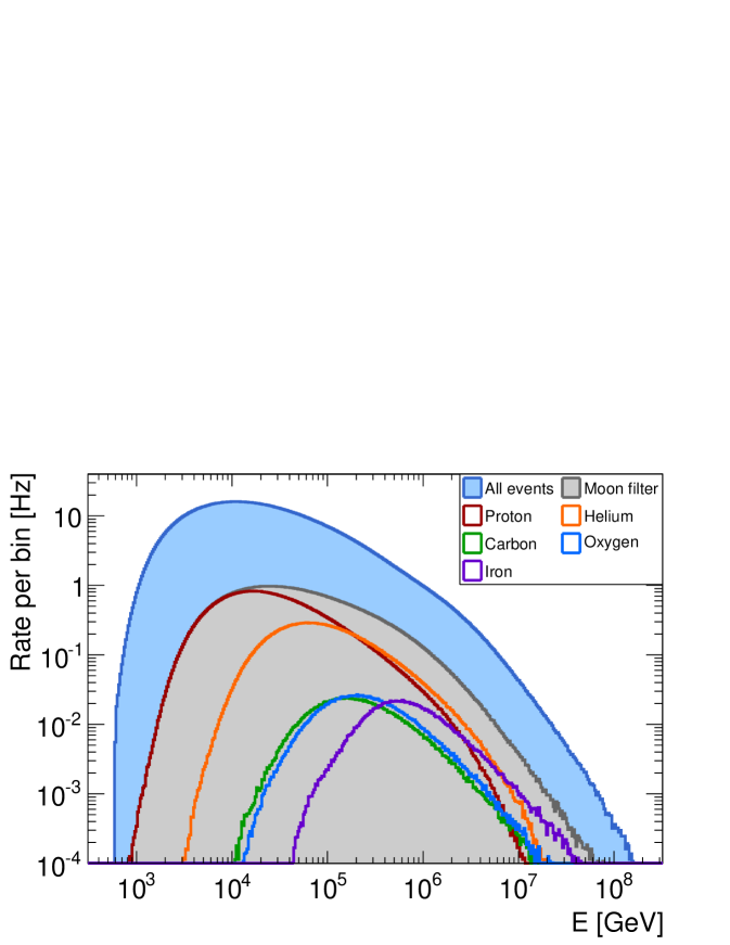
The energy spectrum of all primary cosmic rays triggering the IceCube detector is shown in Fig. 3 and compared to the spectrum of those that pass the Moon filter. Also shown in the figure are the five main chemical elements (protons, He, C, O, and Fe) that make more than 95% of the Moon filter data sample assuming the polygonato composition model. The two main components of the sample are proton (68% of the events) and helium (23%).
III.2 Geomagnetic field effects
Cosmic rays with TeV energies should experience a small deflection in their trajectories due to the influence of the magnetic field of the Earth as they propagate towards the detector. This deflection would appear in the Moon shadow analysis as a shift in the position of the shadow with respect to the true Moon position, which could be wrongly interpreted as a systematic offset produced by the event reconstruction.
In order to quantify this offset and compare it with any possible shift observed in the data, we have developed a particle propagation code that can be used to trace cosmic rays in the geomagnetic field. Using this code, particles are propagated radially outwards from the South Pole up to a a distance of 30 Earth radii from the center of the Earth at which point the opening angle between the initial and final velocity vectors is computed. This angle gives the magnitude of the deflection in the geomagnetic field.
We use the International Geomagnetic Reference Field (IGRF) model Finlay et al. (2010) to calculate deflections. In this model, the field is calculated using a truncated multipole series expansion. The current revision of the model, IGRF-11, can be used to calculate B-field values through 2015, providing a good coverage of the time range over which the data were taken. The model is accessible through a library of FORTRAN routines called GEOPACK developed by N. Tsyganenko111http://geo.phys.spbu.ru/~tsyganenko/modeling.html.
The IGRF-11 model describes what is known as the internal magnetic field of the Earth, which is presumably produced by electric currents in the outer core of the planet and accounts for most of the total magnetic field. A weaker component, known as the external field, is produced by electrical currents in the ionosphere. The external component is not included in our calculation since it only modifies the total angular deflection by a few percent while significantly increasing the computation time needed to perform the simulation.
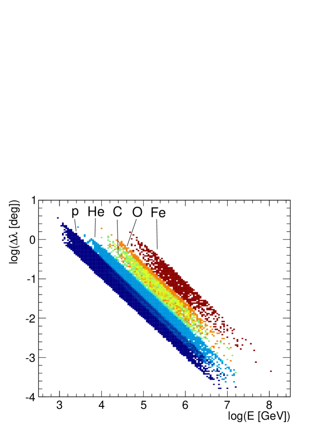
In our simulation, primary cosmic rays are propagated in the direction of the Moon as seen from the South Pole for different times during the data taking period. The cosmic ray energy and chemical composition is sampled from the event distributions that pass the Moon filter, shown in Fig. 3. The resulting total deflection is shown in Fig. 4 as a function of energy for simulated cosmic ray particles for the five main chemical elements that contribute to the Moon dataset. The energy and charge dependence of the deflection angle is evident in the plot. Different bands in the plot correspond to different chemical elements. The width of each band is due to particles that were propagated in different directions in the sky (i.e. through different regions of the Earth’s magnetic field) experiencing different deflections. A power-law fit to the simulation results has been performed to estimate the deflection angle as a function of energy and charge. The fit gives a good agreement for the following expression:
| (1) |
where is the CR charge in units of elementary charge , is its energy in TeV, and is given in degrees. This expression has the same functional form as the one found in Sciascio and Iuppa (2011) with a higher normalization in our simulation, which could be due to the difference in geographic location and other simulation details.
The deflection of each cosmic ray with arrival direction in sidereal coordinates is calculated with respect to the position of the Moon at the time of the event . The two coordinates that characterize the position of an event in this system are a right ascension difference , and a declination difference with respect to the nominal Moon position. The median shift in right ascension for all CR particles in our simulation is , with 68% of the particles having deflection angles in the interval . The median shift in declination is consistent with , with 68% of the events contained in the interval .
The cosmic-ray muons that ultimately trigger IceCube are also deflected by the geomagnetic field. However, since their total track length is in the 50-100 km range and their energy is about 2 TeV, their contribution to the total deflection angle should be at most . For this reason, the muon contribution has been ignored in calculating the expected total deflection angle.
IV Binned analysis
IV.1 Description of the method
The main goal of the binned analysis is to obtain a profile view of the Moon shadow and measure its width, which can be used as a direct estimator of the angular resolution of the event reconstruction. This is accomplished by comparing the observed number of events as a function of angular distance from the Moon to an estimate of how many events would have been observed if there was no shadow.
For this comparison, the angular distance between the reconstructed muon tracks and the expected position of the Moon is binned in constant increments of up to a maximum angular distance of . This defines the so-called on-source distribution of events. The same binning procedure is applied to eight off-source regions centered around points located at the same declination as the Moon, but offset from it in right ascension by , , , and , where it is assumed that the shadowing effect is negligible. The average number of counts as a function of radius for these eight off-source regions represents the expectation in the case of no Moon shadow.
The relative difference between the number of events in the -th bin in the on-source region , and the average number of events in the same bin in the off-source regions is calculated using the following expression:
| (2) |
The uncertainty in the relative difference is given by:
| (3) |
where is the number of off-source regions. The distribution of relative differences as a function of angular radius from the Moon constitutes a profile view of the shadow.
Simulation studies indicate that the point spread function (PSF) of the detector can be approximated with a two-dimensional Gaussian function. We use this approximation to obtain an estimate of the angular resolution of the track reconstruction by fitting the distribution of for the events in the Moon data set.
Following Cobb et al. (2000), we treat the Moon as a point-like cosmic ray sink that removes events from the muon sample, where is the angular radius of the Moon () and is the cosmic ray flux at the location of the Moon in units of events per square degree. This deficit is smeared by the PSF of our detector, which results in radially-symmetric two-dimensional Gaussian distribution of shadowed events which is a function of radial distance from the center of the Moon. Integrating over the azimuthal coordinate of the symmetric Gaussian distribution yields:
| (4) |
where is the angular resolution of the directional reconstruction. The number of shadowed events in the -th bin of width is given by the two-dimensional integral:
| (5) | |||||
| (6) |
The number of events that would have been observed in the same bin with no shadowing is .
The ratio of equations 6 and gives us the expected distribution of relative differences for a detector with a Gaussian PSF of angular resolution :
| (7) |
This expression is used to fit the experimental data, and the resulting value of is compared to an estimate of the angular resolution of the data set obtained from simulation studies. Our treatment ignores the finite angular size of the lunar disc, which may affect the result of the fit. However, for the expected angular resolution of the Moon data set (of order or less) this effect should influence the fit value of only at the few-percent level.
A set of cuts was developed to optimize for the statistical significance of the detection of the Moon shadow. Under the assumption of Poisson statistics, the relation between the significance , the fraction of events passing the cuts, and the resulting median angular resolution after cuts is:
| (8) |
The optimization of the cuts was performed on the CORSIKA-simulated air showers described in Section III. Two cut variables were used in this analysis: the angular uncertainty in the reconstruction of the muon track direction estimated individually for each event, and the reduced log-likelihood , which is the log-likelihood for the best track solution divided by the number of degrees of freedom in the fit. The number of degrees of freedom in the track fit is equal to the number of DOMs triggered by the event minus the number of free parameters in the fit (five for this fit.) Both and are standard cut variables used in the search for point-like sources of astrophysical neutrinos Abbasi et al. (2011b), the search for a diffuse flux of high-energy neutrinos Abbasi et al. (2011c), and several other analyses of IceCube data.
Once the cuts have been determined, the number of events falling inside a circular search bin around the Moon is compared to the number of events contained in a bin of the same angular radius for the average off-source region. The statistical significance of an observed deficit in the number of events in the search bin is calculated using the method given by Li and Ma (1983).
The optimal radius of the search bin can be found by maximizing the parameter in the following expression:
| (9) |
where is the radius of the bin and is the point spread function of the detector after cuts obtained from simulations. Due to its symmetry, the PSF has already been integrated over the azimuthal coordinate and only the radial dependence remains. The optimization of the search bin radius is also performed using simulated CORSIKA showers generated for each detector configuration.
IV.2 Results
A set of cuts was determined independently for both the IC40 and IC59 detector configurations using the optimization procedure described above on simulated data. For IC40, only events with and were used in the analysis, with 26% of the events surviving the cuts. After cuts, the median angular resolution of the reconstruction was estimated from simulation to be , with 68% of the events having angular uncertainties between and . A two-dimensional fit to the simulated data shows that for the Gaussian approximation the corresponding resolution is about .
In the case of IC59, the events selected for the analysis were those with and , which resulted in a passing rate of 34%. The median resolution after cuts was , with the 68% containing interval located between and , with a Gaussian width of about .
After the cuts were applied to both data sets, the radius of the optimal search bin () and the number of events contained in that bin for both the on-source (), and off-source () windows were calculated. In both detector configurations, a deficit in the number of events in the on-source bin when compared to the off-source bin was observed at high statistical significance (), as expected due to the shadowing effect of the Moon. A complete list of the number of events observed on each bin, the observed deficit in the on-source bin, as well as the statistical significance associated with such deficit is given in Table 1.
| IC40 | IC59 | |
|---|---|---|
| 52967 | 96412 | |
| 54672 | 100442 | |
| -1705 | -4030 | |
| Significance |
The Moon shadow profile shown in Fig. 5 was fit using the expression given in Eq. 7, where is the only free parameter. A list of fit results is given in Table 2. In both cases, the observed angular resolution shows good agreement with the one obtained from the above-mentioned simulation studies.
| IC40 | IC59 | |
|---|---|---|
| 31.4 / 24 | 13.0 / 24 |
V Unbinned analysis
V.1 Description of the method
The second algorithm used to search for the Moon shadow is based on an unbinned maximum likelihood method analogous to that used in the search for point-like sources of high-energy neutrinos Braun et al. (2008). This kind of likelihood analysis was first proposed in Kinnison et al. (1982), and was applied for the first time to a Moon shadow search in Wascko (2001).
The goal of the unbinned analysis is to determine the most likely location of the Moon shadow to compare it with the expected location after accounting for magnetic deflection effects. An agreement between the observed and expected positions of the shadow center will serve as an important confirmation of the absolute pointing accuracy of the detector.
The analysis is also used to obtain the most likely number of events shadowed by the Moon, which can be compared to the expectation. An essential ingredient in the unbinned analysis is an event-wise estimation of the angular error. Both systematic under- and overestimation of this error would lead to a shallower apparent shadow than expected. The number of shadowed events is a free parameter in this analysis and the comparison with the expected number of shadowed events is effectively a test of the angular uncertainty estimate.
In this analysis Blumenthal (2011); Reimann (2011), the position of each muon event is defined with respect to the Moon position in the coordinate system that was defined in Section III.2. Only events with and were considered in the analysis, where defines the on-source region, and define two off-source regions.
A set of quality cuts was determined for this analysis using the same simulation dataset as in the one-dimensional binned case. The same variables were used in the optimization of the cuts: the angular reconstruction uncertainty , and the reduced log-likelihood of each event rlogl.
The analysis method assumes that the data can be described as a linear combination of signal and background components, where the relative contribution from each component is established by a maximum likelihood fit to the data. For a data set containing events, the log-likelihood function is defined as
| (10) |
where and are the signal and background probability density functions (PDFs), is the unknown number of signal events, or in this case the total number of shadowed events, and is the unknown central position of the shadow of the Moon, relative to the nominal position of the Moon. Note that since the expected signal in the case of the Moon is a deficit in the muon flux rather than an excess, should be negative. In absence of a geomagnetic field, the shadow should occur exactly on the nominal position of the Moon, i.e. , but according to the estimates described in section III.2 we expect the shadow to be shifted by about .
Other potential sources of systematic errors could also produce a shift or a smearing of the shadow. For example, it is expected that the timing accuracy of IceCube should be better than 1 s, but if due to a detector malfunction a systematic error of a few minutes were introduced in the event registration time, the observed position of the shadow would experience a shift of order . A similar effect would be observed if the detector geometry used for reconstructions differed from the real one by several meters, or if the properties of light propagation in the ice Aartsen et al. (2013) induced a systematic shift in the reconstructed direction of the muon tracks. In fact, a measurement of the shadow of the Moon with the expected location, depth and width serves as an independent verification that all these possible systematical errors are indeed under control.
The signal PDF for each event is modeled using a two-dimensional Gaussian distribution around the reconstructed direction of the muon track:
| (11) |
where the width of the Gaussian distribution is the angular reconstruction uncertainty obtained on an event-by-event basis by the paraboloid algorithm described in Section II.2.
The background PDF is assumed to depend only on , and is derived from the distribution of reconstructed declination angles for the muon tracks contained in the two off-source regions.
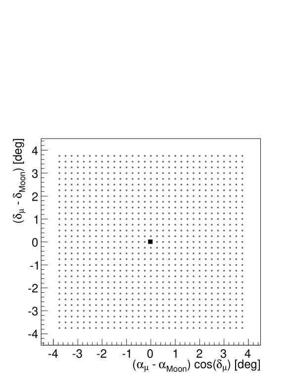
The best fit values for the number of signal events in the data and the shift of the shadow center are determined by maximizing the log-likelihood function (10). Besides and also the width and overall shape of the shadow are of interest. In searches for point sources of high-energy neutrinos Braun et al. (2008), for all points on a fine grid covering the sky, the value of is determined which maximizes the likelihood function. Similarly, in the Moon shadow analysis we determine the value of that maximizes the likelihood function (10) on a rectangular grid of 961 values for . This 3131 grid is defined inside a window with a size of and shown in Fig. 6 .
In order to avoid edge effects, all events in the on-source region are taken into account in the maximum likelihood calculation.
The statistical significance associated with each value of can then be calculated by applying the same likelihood analysis to the two off-source regions. The RMS spread of the resulting distribution of values for those regions gives an estimate of the spread expected in the case of a null detection. Using this estimate, each point in the on-source region can be given a statistical significance by taking the ratio between the value of at that point and the estimate from the off-source regions.
The observed value of is compared to an estimate of the true number of CRs shadowed by the Moon. This estimate is obtained by counting the number of events that fall within a circular window with the same radius as the Moon but located in the off-source region.
| IC40 | IC59 | |
|---|---|---|
| Events before cuts | 18.8 | 22.2 |
| Cut 1: | ||
| Cut 2: rlogl | ||
| Events after cuts | 8.4 | 11.7 |
V.2 Results
V.2.1 SPE analysis
The cuts used in the unbinned analysis are listed in Table 3 . The resulting median angular resolution of the IC40 and IC59 data sets was estimated by applying those same cuts to simulated cosmic-ray events. In the case of IC40, the median angular resolution is , with 68% of the events having angular uncertainties between and . For IC59, the median resolution is , with a 68% containing interval defined between and .
| IC40 | IC59 | |
|---|---|---|
| Observed deficit | ||
| Expected deficit | ||
| Off-source RMS | 521 | 627 |
| Significance | ||
As described in the previous section, the maximum-likelihood values of were calculated on a grid around the position of the Moon for both sets. The contour maps of the values obtained for IC40 and IC59 are shown in Fig. 7, where the shadowing effect of the Moon is visible as a strong deficit in the central regions of the maps. The deepest deficit observed with both detector configurations is in good agreement with the expected number of shadowed events, listed in Table 4. Using the RMS spread of the off-source regions as a estimator in the case of a null detection, we calculated the statistical significance of the observation by taking the ratio of the largest deficit observed to the RMS spread, which is also shown in Table 4. The shadow of the Moon is observed in both the IC40 and IC59 datasets to high statistical significance ().
In order to obtain a better estimate of the position of the minimum of the shadow, a finer grid with a spacing of about was used in the central region around the Moon. Using this grid, we obtain the positions indicated in Table 4 as offsets in right ascension () and declination () with respect to the nominal position of the Moon in the sky. The shadow positions for both detector configurations are shown in Fig. 8 together with , , and contours. The expected location of the minimum after accounting for geomagnetic deflection effects is also given for comparison. In both detector configurations, the observed position of the minimum is consistent with its expected location to within statistical fluctuations. These measurements imply that the absolute pointing accuracy of the detector during the IC40 and IC59 data-taking periods was better than about .
V.2.2 MPE analysis
The unbinned analysis was also applied to IC59 events reconstructed using the MPE algorithm and its corresponding angular error estimate described in Section II.2. In simulations, the MPE fit performs better than the SPE reconstruction thanks to its more realistic description of the arrival times of multiple photons at each DOM. However, at high energies the algorithm can be confused by stochastic energy losses that occur along the muon track and are not described in the likelihood function implemented in the MPE algorithm. This usually results in an underestimation of the angular uncertainty on the reconstructed direction of the track. In practice, this problem can be solved by rescaling the average pull (the ratio between the real and estimated angular errors as obtained from simulation studies) to unity. The MPE version of the unbinned analysis was used as a verification of this correction technique.
Simulation studies indicate an average pull of 1.55 for the MPE reconstruction, versus 1.0 for SPE. Without correcting for this underestimation of the angular error in the MPE fit, the Moon shadow analysis resulted in a minimum value for of shadowed events, differing by more than 5 standard deviations from the expectation of . Redoing this analysis with the angular error estimates rescaled by a factor of 1.55 resulted in fitted value compatible with expectation, validating the pull correction method.
In neutrino analyses, where the range of muon energies is much larger than in the Moon analysis sample, the applied MPE pull correction is energy-dependent, instead of using only the average value of the pull for the entire data set.
VI Conclusions
The shadow of the Moon in TeV cosmic rays has been detected to high significance () using data taken with the IC40 and IC59 configurations of the IceCube Neutrino Observatory. For both detector configurations, the observed positions of the shadow minimum show good agreement with expectations given the statistical uncertainties. An important implication of this observation is that any systematic effects introduced by the detector geometry and the event reconstruction on the absolute pointing capabilities of IceCube are smaller than about .
The average angular resolution of both data samples was estimated by fitting a Gaussian function to the shadow profile. In both cases, the width of the Moon shadow was found to be about , which is in good agreement with the expected angular resolution based on simulation studies of down-going muons.
The total number of shadowed events estimated using the unbinned analysis is also consistent with expectations for IC40 and IC59. This provides an indirect validation of the angular uncertainty estimator obtained from the reconstruction algorithm. This is especially relevant for the MPE analysis, where simulation studies indicate that the uncertainty estimator has to be rescaled in order to avoid underestimating the true angular error. Applying this correction factor to the data results in a number of shadowed events compatible with expectation.
Note that the value of the average angular resolution determined in this analysis is not a direct measurement of the point spread function to be used in searches for point sources of high-energy neutrinos. Rather, the agreement of this value with the value estimated from our simulations should be seen as an experimental verification of our simulation and the methods used to estimate the angular uncertainty of individual track reconstructions. This angular uncertainty depends on several factors, in particular on the energy with which the muon traverses the detector. As the energy distribution for neutrino analyses differs from that of the Moon shadow analysis, the average angular resolution may be better or worse, but can reliably be estimated from our simulation.
Acknowledgements.
We acknowledge the support from the following agencies: U.S. National Science Foundation-Office of Polar Programs, U.S. National Science Foundation-Physics Division, University of Wisconsin Alumni Research Foundation, the Grid Laboratory Of Wisconsin (GLOW) grid infrastructure at the University of Wisconsin - Madison, the Open Science Grid (OSG) grid infrastructure; U.S. Department of Energy, and National Energy Research Scientific Computing Center, the Louisiana Optical Network Initiative (LONI) grid computing resources; Natural Sciences and Engineering Research Council of Canada, WestGrid and Compute/Calcul Canada; Swedish Research Council, Swedish Polar Research Secretariat, Swedish National Infrastructure for Computing (SNIC), and Knut and Alice Wallenberg Foundation, Sweden; German Ministry for Education and Research (BMBF), Deutsche Forschungsgemeinschaft (DFG), Helmholtz Alliance for Astroparticle Physics (HAP), Research Department of Plasmas with Complex Interactions (Bochum), Germany; Fund for Scientific Research (FNRS-FWO), FWO Odysseus programme, Flanders Institute to encourage scientific and technological research in industry (IWT), Belgian Federal Science Policy Office (Belspo); University of Oxford, United Kingdom; Marsden Fund, New Zealand; Australian Research Council; Japan Society for Promotion of Science (JSPS); the Swiss National Science Foundation (SNSF), Switzerland.References
- Abbasi et al. (2013) R. Abbasi et al. (IceCube Collaboration), Phys. Rev. D 87, 012005 (2013), arXiv:1208.2979 [astro-ph.HE] .
- Abbasi et al. (2010a) R. Abbasi et al. (IceCube Collaboration), The Astrophysical Journal Letters 718, L194 (2010a), arXiv:1005.2960 [astro-ph.HE] .
- Abbasi et al. (2011a) R. Abbasi et al. (IceCube Collaboration), The Astrophysical Journal Letters 740, 16 (2011a), arXiv:1105.2326 [astro-ph.HE] .
- Clark (1957) G. W. Clark, Phys. Rev. 108, 450 (1957).
- Ambrosio et al. (2003) M. Ambrosio et al. (MACRO Collaboration), Astroparticle Physics 20, 145 (2003), arXiv:astro-ph/0302586 [astro-ph] .
- Achard et al. (2005) P. Achard et al. (L3 Collaboration), Astroparticle Physics 23, 411 (2005), arXiv:astro-ph/0503472 [astro-ph] .
- Oshima et al. (2010) A. Oshima et al. (GRAPES-3 Collaboration), Astroparticle Physics 33, 97 (2010).
- Adamson et al. (2011) P. Adamson et al. (MINOS Collaboration), Astroparticle Physics 34, 457 (2011), arXiv:1008.1719 [hep-ex] .
- Bartoli et al. (2011) B. Bartoli et al. (ARGO-YBJ Collaboration), Phys. Rev. D 84, 022003 (2011).
- Abbasi et al. (2011b) R. Abbasi et al. (IceCube Collaboration), The Astrophysical Journal 732, 18 (2011b), arXiv:1012.2137 [astro-ph.HE] .
- Abbasi et al. (2010b) R. Abbasi et al. (IceCube Collaboration), Nucl. Instrum. Meth. A618, 139 (2010b), arXiv:1002.2442 [astro-ph.IM] .
- Abbasi et al. (2009) R. Abbasi et al. (IceCube Collaboration), Nucl. Instrum. Meth. A601, 294 (2009), arXiv:0810.4930 [physics.ins-det] .
- Abbasi et al. (2012) R. Abbasi et al. (IceCube Collaboration), Astroparticle Physics 35, 615 (2012), arXiv:1109.6096 [astro-ph.IM] .
- Ahrens et al. (2004) J. Ahrens et al. (AMANDA Collaboration), Nucl. Instrum. Meth. A524, 169 (2004), arXiv:astro-ph/0407044 .
- Wallace (1994) P. Wallace, ASP Conf. Ser. 61, 481 (1994).
- Meyers and Shore (1989) R. A. Meyers and S. N. Shore, eds., Encyclopedia of Astronomy and Astrophysics (Academic Press, 1989).
- Neunhöffer (2006) T. Neunhöffer, Astroparticle Physics 25, 220 (2006), arXiv:astro-ph/0403367 [astro-ph] .
- Heck et al. (1998) D. Heck et al., CORSIKA: A Monte Carlo Code to Simulate Extensive Air Showers, Tech. Rep. FZKA 6019 (Forschungszentrum Karlsruhe, 1998).
- Ahn et al. (2009) E.-J. Ahn et al., Phys. Rev. D80, 094003 (2009), arXiv:0906.4113 [hep-ph] .
- Hörandel (2003) J. R. Hörandel, Astropart. Phys. 19, 193 (2003), arXiv:astro-ph/0210453 .
- Finlay et al. (2010) C. C. Finlay et al., Geophys. J. Int. 183, 1216 (2010).
- Sciascio and Iuppa (2011) G. D. Sciascio and R. Iuppa, Nucl. Instrum. Meth. A630, 301 (2011), proceedings of the 2nd Roma International Conference on Astroparticle Physics (RICAP 2009).
- Cobb et al. (2000) J. H. Cobb et al. (Soudan 2 Collaboration), Phys. Rev. D 61, 092002 (2000), arXiv:hep-ex/9905036 [hep-ex] .
- Abbasi et al. (2011c) R. Abbasi et al. (IceCube Collaboration), Phys. Rev. D 84, 082001 (2011c).
- Li and Ma (1983) T.-P. Li and Y.-Q. Ma, Astrophys. J. 272, 317 (1983).
- Braun et al. (2008) J. Braun, J. Dumm, F. D. Palma, C. Finley, A. Karle, and T. Montaruli, Astroparticle Physics 29, 299 (2008), arXiv:0801.1604 [astro-ph] .
- Kinnison et al. (1982) W. W. Kinnison et al., Phys. Rev. D 25, 2846 (1982).
- Wascko (2001) M. Wascko, Study of the Shadow of the Moon in Very High Energy Cosmic Rays with the Milagrito Water Cherenkov Detector, Ph.D. thesis, University of California, Riverside (2001).
- Blumenthal (2011) J. Blumenthal, Measurements of the Shadowing of Cosmic Rays by the Moon with the IceCube Neutrino Observatory, Diploma thesis, Rheinisch-Westfälische Technische Hochschule (RWTH) Aachen (2011).
- Reimann (2011) R. Reimann, Untersuchungen mit Graphik-Prozessoren (GPU) zur Messung der Abschattung kosmischer Strahlung durch den Mond in IceCube, Diploma thesis, Rheinisch-Westfälische Technische Hochschule (RWTH) Aachen (2011).
- Aartsen et al. (2013) M. G. Aartsen et al. (IceCube Collaboration), Nucl. Instrum. Meth. A711, 73 (2013), arXiv:1301.5361 [astro-ph.IM] .