Observing Black Hole Phase Transitions in Extended Phase Space and Holographic Thermodynamics Approaches from Optical Features
Abstract
The phase transitions of charged Anti-de Sitter (AdS) black holes are characterized by studying null geodesics in the vicinity of the critical curve of photon trajectories around black holes as well as their optical appearance as the black hole images. In the present work, the critical parameters including the orbital half-period , the angular Lyapunov exponent , and the temporal Lyapunov exponent are employed to characterize black hole phase transitions within both the extended phase space and holographic thermodynamics frameworks. Under certain conditions, we observe multi-valued function behaviors of these parameters as functions of bulk pressure and temperature in the respective approaches. We propose that , , and can serve as order parameters due to their discontinuous changes at first-order phase transitions. To validate this, we provide detailed analytical calculations demonstrating that these optical critical parameters follow scaling behavior near the critical phase transition point. Notably, the critical exponents for these parameters are found to be , consistent with those of the van der Waals fluid. Our findings suggest that static and distant observers can study black hole thermodynamics by analyzing the images of regions around the black holes.
I Introduction
Thermodynamics of black holes (BHs) has emerged as an active research area that offers deep insights into the interplay among gravity, thermodynamics, quantum mechanics, and information theory. Initiated by Bekenstein [1] and Hawking [2], the energy , entropy and temperature of a BH can be written in the geometric description as follows
| (1) |
where , and are the mass of BH, the surface area of event horizon, and surface gravity at the event horizon, respectively. With such geometric identification, the laws of BH mechanics [3] and the laws of thermodynamics exhibit a surprising mathematical analogy, leading us to consider BHs as thermal objects.
The discussion of BH thermodynamics has been significantly enriched by the discovery of holographic descriptions. Given that the symmetry group of and the conformal group in -dimensional spacetime are both isomorphic to , the AdS/CFT correspondence emerged as a duality between the gravitational system in the bulk AdS space and the conformal field theory (CFT) on the boundary [4, 5, 6, 7]. Specifically, thermal radiation and BHs within an -dimensional AdS space respectively correspond to the -dimensional confining phase at zero temperature and thermal states within the deconfining phase of the large- gauge theory. Consequently, the confinement-deconfinement phase transition in gauge theory has the gravitational description in the bulk through the Hawking-Page phase transition of AdS-BHs [8].
Despite significant advancements, several issues in BH thermodynamics remain unresolved. The first issue involves the Smarr formula [9], which expresses the relation between different geometric quantities of a BH in the same fashion as the Euler equation in conventional thermodynamics. However, there is an additional term in the Smarr formula when considering BHs with a nonzero cosmological constant . The Smarr formula for AdS-BH is given by:
| (2) |
where is the angular velocity, is the angular momentum, is the electric potential and is the electric charge of BH. Note that has been suggested to be defined as the proper volume weighted locally by a Killing vector [10]. Despite this formulation, there continues to be significant debate over the appropriate thermodynamic interpretation of and its conjugate variable . The second issue arises from the observation that the first law of BH thermodynamics does not include the term. As a result, one may wonder whether the holographic description can provide a gravitational description of the mechanical work term dual to that of the conformal matter.
Remarkably, there are two recent progresses that can be applied to resolve these important issues as follows.
-
•
Black hole chemistry or extended phase space approach is an extension of thermodynamic phase space for AdS-BHs by identifying the negative cosmological constant and its conjugate variable as a bulk pressure and thermodynamic volume via
(3) where for spherical symmetric BHs [11, 12, 13, 14], for good reviews see [15, 16] and reference therein. In this way, the first law of BH thermodynamics has additional work term, so the BH’s mass should be identified as an enthalpy rather than the internal energy of the BH. Notably, the extended phase space approach gives a more consistent gravitational analog of the first law of thermodynamics in conventional matter. For example, the Hawking-Page phase transition in Schwarzschild AdS can be interpreted as solid-liquid phase transition [17], isotherm curves in plane of charged AdS-BH in canonical ensemble undergoes a family of Small-Large BHs first order phase transition ending at a critical point of second order phase transition corresponds to the liquid-gas phase transition in the van der Waals (vdW) fluid [18, 19, 20] and the Small-Large-Small BHs phase transition occurs in rotating and nonlinear electrodynamics AdS-BHs analogous to the reentrant phase transition of multicomponent liquids [21, 22]. Moreover, this framework introduces what can be referred to as the black hole’s molecules for black hole thermodynamics [23, 24, 25]. These entities can serve similarly to the microscopic constituents in statistical mechanics, providing a means to describe thermodynamic behavior.
-
•
Holographic thermodynamics has been proposed to address concerns about the consistency of the extended phase space approach with the AdS/CFT correspondence. Although the extended phase space approach provides a plausible interpretation of and its conjugate for describing the thermodynamics of AdS-BHs, its consistency with the AdS/CFT correspondence remains debated by some researchers [26, 27, 28, 29, 30]. Before discussing progress in holographic thermodynamics aimed at resolving these consistency issues, let us first clarify two important points within the extended phase space approach that continue to be questioned. They are as follows:
-
(i)
The equation of state for conformal fluid with energy , pressure and volume is described by
(4) According to the AdS/CFT dictionary, of -dimensional conformal fluid is holographically dual to the mass of BH in -dimensional spacetime. It is evident that upon replacing and in the above equation with and in Eq. (3) respectively, the result indicates that is not equal to of the BH. This implies that the bulk pressure and the volume for BH are not equivalent to the fluid’s pressure and volume . In other words, the Smarr relation of BHs in the bulk does not correspond to the Euler equation of large- gauge theories on the boundary.
-
(ii)
In fact, the AdS/CFT correspondence suggests that should be dual to the number of colors in the large- gauge theory via the relation [30]
(5) where is the central charge and is the constant depending on the details of a particular system. These relations suggest that the variation of implies a variation of , which is the rank of the gauge group. Therefore, varying of the bulk leads to changing from one field theory to another. Moreover, the variation of also corresponds to variation in the volume of the dual gauge theory since the geometry of dual field theory depends on of the bulk.
Visser [31] proposed an approach to overcome this issue, demonstrating that the Euler equation of the dual field theory requires the term but lacks the term, while the term appears in the first law of thermodynamics. Here, and are the central charge and its chemical potential, respectively. On the gravity side, introducing and as thermodynamic variables in the boundary theory is equivalent to allowing for variations in both the Newton constant and the AdS radius in the bulk theory. Using Eq. (5), it becomes possible to vary both and while keeping fixed at the boundary, ensuring the field theory remains unchanged to another. Thus, one can more appropriately study the variations in the volume of the dual field theory as changes. As suggested in [31], the terms and in Eq. (2) can be rewritten in terms of and . This leads to consistency between the Smarr formula and the Euler equation within the framework known as holographic thermodynamics. Recently, the thermodynamic behaviors resulting from holographic thermodynamics have been extensively studied [32, 33, 34, 35, 36, 37, 38]. For a comprehensive recent review, see [39].
-
(i)
While BH thermodynamics has been developed with intriguing arguments as discussed above, determining the most valid approach remains challenging. It is crucial to support theoretical claims with observations or at least establish a connection between them. It makes sense to argue that the thermal properties of BHs should manifest in specific observational signatures. A natural question that arises is how we can obtain proper observational signatures of a BH to identify its thermodynamic properties and phase transitions. Unfortunately, the observational confirmation of BH thermodynamics remains difficult, although recent advancements that have provided evidence of BH existence through the gravitational wave (GW) signal emitted by a binary black hole (BBH) [40] and the images of two supermassive BHs, i.e., M87* and SgrA* [41, *ETH2, *ETH3, *ETH4, *ETH5, *ETH6, *EventHorizonTelescope:2022wkp, *EventHorizonTelescope:2022apq, *EventHorizonTelescope:2022wok, *EventHorizonTelescope:2022exc, *EventHorizonTelescope:2022urf, *EventHorizonTelescope:2022xqj]. More specifically, the thermodynamic quantities of BHs are typically defined via their event horizons, which are difficult to detect directly from observers at asymptotic infinity.
Although the AdS-BH seems to be interested only in the theoretical aspect, it is valuable to find ways to connect its thermodynamic behaviors with observational signatures. Numerous studies on AdS-BH have attempted to relate the BH phase transition to some signals, which can be observed at asymptotic infinity. Namely, the quasinormal modes (QNMs), which can be characterized by the signature in the GWs emitted from a BH during the ringdown stage [53, 54, 55, 56] and null geodesics of test particles moving near the BH [57, 58, 59, 60, 61]. Recently, the geodesic instability of test particles, specifically focusing on the temporal-Lyapunov exponents of both massless and massive particles, serving as an order parameter to investigate phase transitions in numerous BH solutions in asymptotically AdS spacetime [62, 63, 64, 65, 66].
Strong gravitation near a BH can cause photons traveling close to the critical curve to orbit the BH multiple times before reaching a distant observer, forming a narrow band on the observer’s screen known as the photon ring. This ring can be characterized by three critical parameters: the orbital half-period (), the angular-Lyapunov exponent (), and the temporal-Lyapunov exponent (), which govern the dynamics of unstable null geodesics and reveal universal properties of the photon ring independent of the distance between the light source and observer from the BH [67, 68] as well as the feature of the emitting light source. In this study, we focus on these observable parameters to decode information about the phase transitions of BHs, particularly charged AdS-BHs, within the framework of extended phase space and holographic thermodynamics. Moreover, we propose that the differences in these three critical parameters at first-order phase transitions could serve as an order parameter for studying scaling behavior near the critical point, and we also provide a mathematical derivation for the corresponding scaling law.
This paper is organized as follows: In section II, we provide a comprehensive review of BH thermodynamics, focusing on three approaches: standard phase space, extended phase space, and holographic thermodynamics. This section sets the stage for our analysis by detailing the theoretical foundations and the distinctions between these approaches. In section III, we introduce three critical parameters of the photon ring region. We discuss the orbital half-period , the angular Lyapunov exponent , and the temporal Lyapunov exponent , explaining their significance in probing BH phase transitions with horizon-scale observations. Section IV examines the phase transitions of BHs through optical features in the extended phase space and holographic thermodynamics approaches. We analyze how the critical parameters vary with changes in the pressure and temperature, and demonstrate their potential as order parameters indicating phase transitions. In section V, we investigate the scaling behavior of the optical parameters near the critical point within both the extended phase space and holographic thermodynamics approaches. We explore the critical exponents and their implications for understanding BH phase transitions. The results of this investigation support the use of these optical critical parameters as order parameters for characterizing BH phase transitions. Finally, section VI concludes the paper by summarizing our findings and discussing the broader implications of our study for BH thermodynamics and observational astrophysics.
II Many facets of black hole thermodynamics
In this section, we provide a comprehensive review of the thermodynamics of charged AdS-BHs using three approaches: standard phase space, extended phase space, and holographic thermodynamics. The insights gained here will inform our analysis of null geodesics near the critical curve, which may reflect the phase transitions of black holes within each thermodynamic framework discussed in section IV.
II.1 Thermodynamics of charged AdS-BH within standard phase space
The action for Einstein-Maxwell gravity in -dimensional AdS spacetime is given by
| (6) |
where is the gauge field strength tensor and is the negative cosmological constant with the length scale of the AdS space . A spherical symmetric BH solution from this action is
| (7) |
where
| (8) |
Note that is the metric of unit sphere. The parameter is related to the mass of BH as follows
| (9) |
where is the volume of the unit sphere. The electric charge of BH can be written in the form of the parameter as
| (10) |
where is given by
| (11) |
For spherical symmetric and static charged BH, one can choose the gauge potential as
| (12) |
Here, is fixed and set to vanish at the horizon surface , so that the electric potential becomes
| (13) |
The Hawking temperature of BH and its corresponding entropy are associated with its geometrical quantities as
| (14) | |||||
| (15) |
where and denote the surface gravity and horizon area, respectively.
Recall that the partition function in the grand canonical ensemble is the Laplace transform of the density of states as follows
| (16) |
where and denote the inverse temperature, internal energy, chemical potential and number of particles in the system, respectively. To obtain the density of states, we apply an inverse Laplace transform to and then use the steepest descent method. Thus, we have
| (17) |
As the thermal entropy defined as the logarithm of the number of states, the above equation can give the grand potential, , in the form of thermodynamic variables as
| (18) |
The first law of thermodynamics satisfies
| (19) |
Thus, we treat and as independent thermodynamic variables so that we can express the grand potential as the function of these three variables, i.e., . Applying the Legendre transformation to obtain the Helmholtz free energy of the canonical ensemble, , we have
| (20) |
With the first law of thermodynamics, the infinitesimal change in reads
| (21) |
In gravitational physics, the partition function of BHs can be approximated from the on-shell Euclidean action as follows [69]
| (22) |
To evaluate the Einstein-Maxwell action in Eq. (6) with the potential fixed at infinity, the Gibbons-Hawking boundary term vanishes due to the strength tensor becoming zero. Consequently, the partition function can be simply calculated from the bulk action without any additional term. Using the subtraction method, the resulting thermodynamic potential is in the form [70, 71, 72]
| (23) |
Comparing Eqs. (18) with (23), one may identify , and of the thermal systems with , and of the charged BH. It is important to note that the thermodynamic potential corresponding to the grand potential , in the above equation, is derived by calculating the on-shell action with potential fixed at the boundary of spacetime. Recall that the potential is given by taking into Eq. (12). Alternatively, the thermodynamic potential corresponding to the Helmholtz free energy can be obtained by fixing the charge at the spacetime boundary instead. In this approach, the Gibbons-Hawking term no longer vanishes but becomes significant and contributes to the on-shell action . The resulting Euclidean action calculation with fixed at the boundary yields the Helmholtz free energy as the corresponding thermodynamic potential:
| (24) |
II.2 Extended phase space approach
As discussed in the previous subsection, it is indeed possible to associate the thermodynamic variables of BH with the geometric properties of its spacetime. However, the Euler’s theorem for a homogeneous function suggests that the Smarr formula in Eq. (2) for BHs in the spacetime with non-zero become inconsistent with the first law of black hole thermodynamics unless variations in are taken into account. Using Eqs. (2) and (3) and allowing for variations in the cosmological constant , we obtain the Smarr formula and the variation of mass in the form
| (25) | |||||
| (26) |
respectively. Note that the computations concerning the Smarr formula and its associated first law derived from the scaling argument are detailed in Appendix A of the manuscript.
As presented in Eq. (26), the BH mass is a function of and , thus it should be interpreted as the enthalpy rather than the internal energy . Using the Legendre transformation , treating to be enthalpy leads to the first law of black hole thermodynamics in the extended phase space of the form
| (27) |
Significantly, the first law can now describe the change in internal energy during processes associated with changes in volume within a black hole’s event horizon when it absorbs energy or emits Hawking radiation through the term, akin to conventional thermodynamics.
Let us consider black hole thermodynamics in the canonical ensemble within the extended phase space approach. Eliminating in Eq. (14) by identifying , we obtain the equation of state for a -dimensional charged AdS-BH as follows [18]
| (28) |
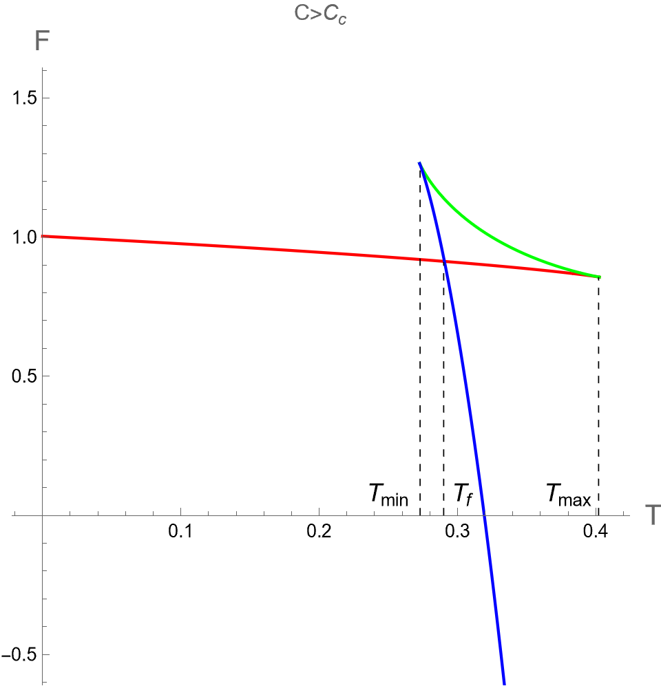
By comparing the above equation with the equation of state for vdW fluids, one can find that relates to the gas’s constant in the vdW equation of state [18]. Using Eq. (28), we plot the isotherm curves for different temperatures, as shown in the left panel in Fig. 1. This depiction presents the critical behavior in the plane. Note that the critical values and of this system satisfy the following conditions:
| (29) |
Solving these two conditions, we obtain
| (30) |
Since should have positive values for , there exists a particular value of temperature which is the lower bound of temperature where at a particular value of horizon radius . Namely,
| (31) |
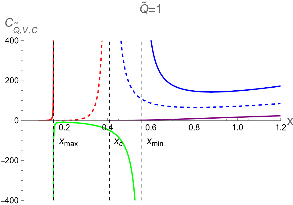
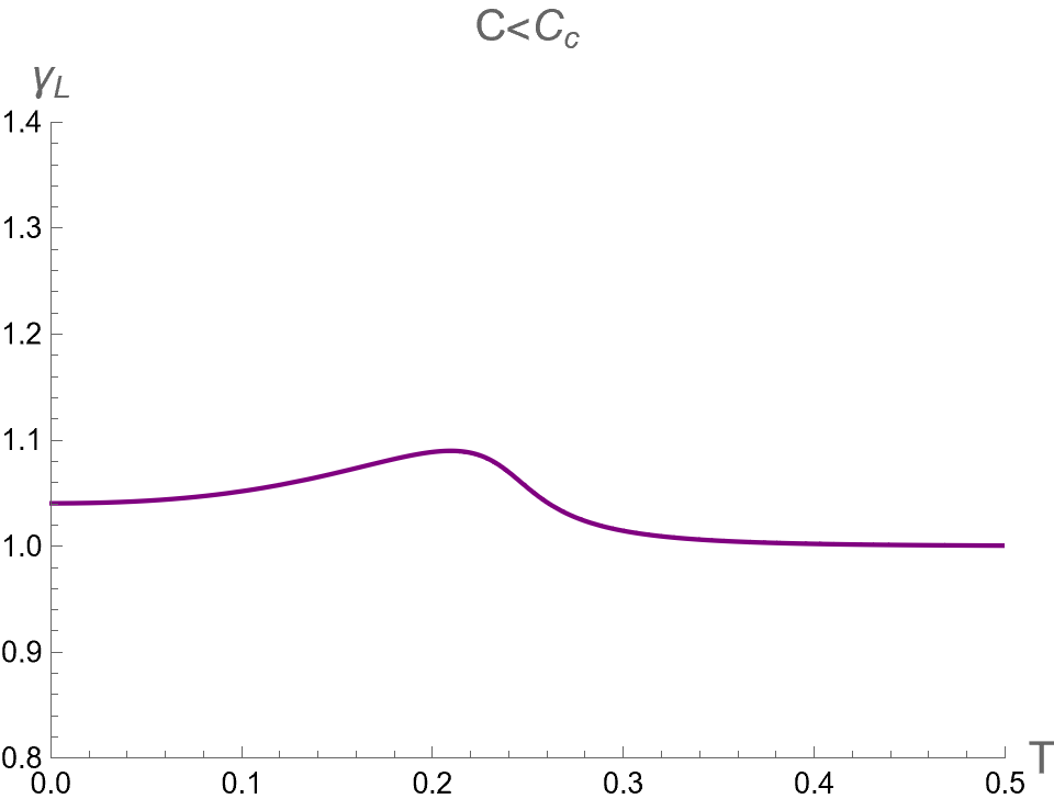
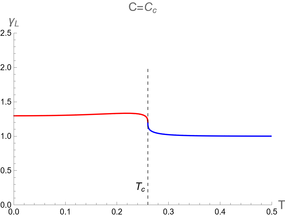
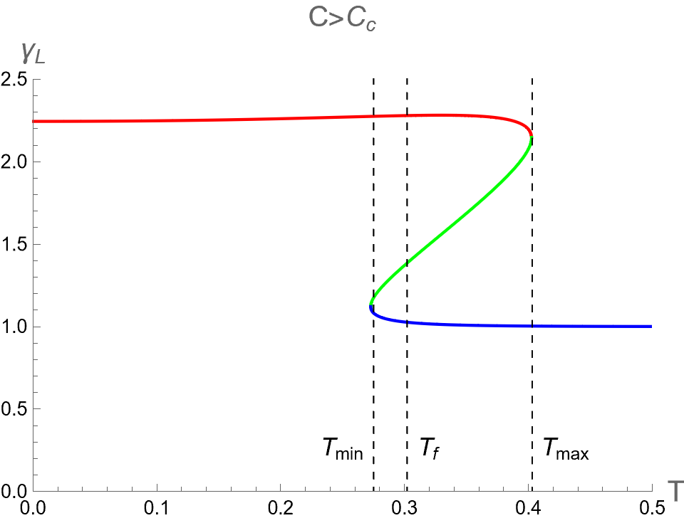
At below , the isotherm curves in the plane show the appearance of a local minimum and a local maximum at the horizon radii and , respectively. Using Eq. (30) and fixing , the critical parameters are given by , , and . To illustrate the characteristics of the system, we present the curves for less than, equal to, and greater than . As shown in Fig. 1, the curves for (below the critical point), , and (above the critical point) are depicted. For , we find that and , corresponding to and , respectively.
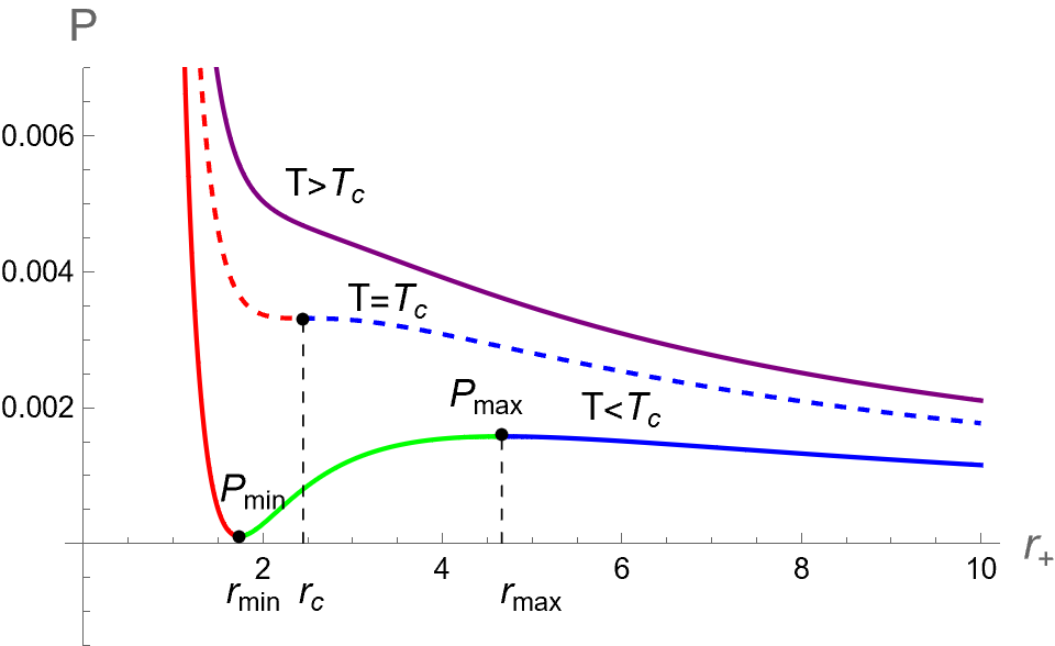
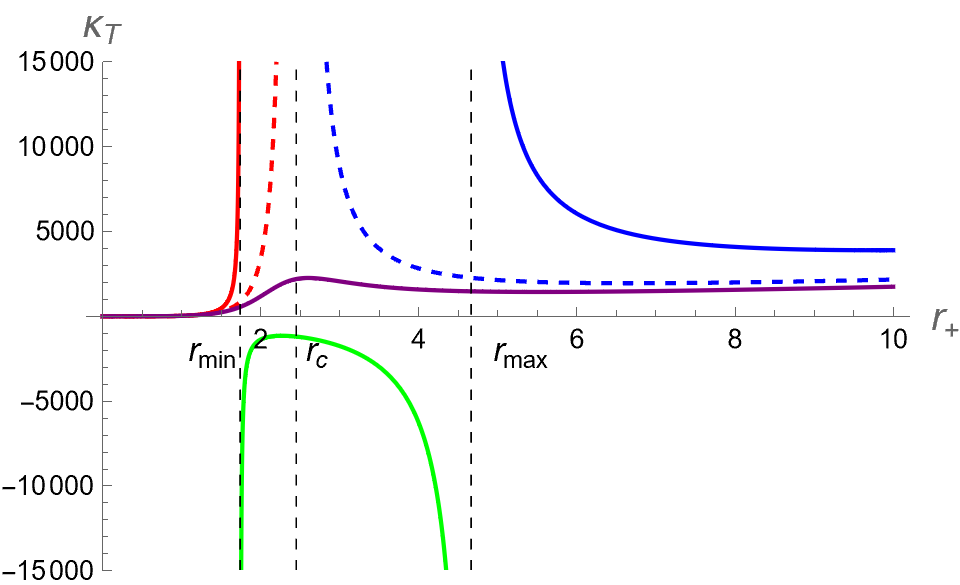
According to the Le Chatelier principle [73, 74, 75, 76], the response function associated to the isotherm curves in plane is the isothermal compressibility , which is defined as
| (32) |
where is thermodynamic volume. The right panel in Fig. 1 displays dependence of corresponding to isotherm curves in plane in the left panel. The results reveal three branches of BHs below : Small BH (red solid curve), Intermediate BH (green solid curve) and Large BH (blue solid curve) correspond to the ranges of and , respectively. Here and is the event horizon radii that diverge. Note that these values of can be obtained by setting the denominator in Eq. (32) to be zero, namely , and finding its roots. The Small BH and Large BH (both have ) are mechanically stable against microscopic fluctuation while the Intermediate BH () is unstable. The authors in [77] have shown that the unstable Intermediate BH in the plane can be replaced by a straight line at obeying the Maxwell equal area law, where the Small-Large BHs first-order phase transition occurs. Note that can be called as the Hawking-Page pressure. Defining the reduced variables as
| (33) |
an analytic expression for Hawking-Page pressure is given by [77]
| (34) |
where denotes the reduced Hawking-Page pressure. Considering the isotherm curve with , for example, which is less than as shown in Fig. 1, the corresponding reduced temperature can be put into the above equation such that the reduced pressure at which the first-order phase transition occurs is at , corresponding to . Moreover, the horizon radii for Small and Large BHs at the first-order phase transition are respectively expressed as follows
| (35) | |||||
| (36) |
where and .
To investigate the global stability for charged AdS-BH associated with the isotherm curves in the plane, one needs to consider the free energy as a function of bulk pressure with the temperature held fixed. In the fixed charge ensemble, treating as the internal energy results in the thermodynamic potential being the Helmholtz free energy , as is typical in standard phase space. However, in this section, where is treated as the enthalpy, the thermodynamic potential is instead the Gibbs free energy . We express in term of with fixed in the following form
| (37) | |||||
By using from Eq. (26) with the charge fixed, the infinitesimal change of the Gibbs free energy is
| (38) |
can be changed to be in the form
| (39) |
This relation suggests that leading to the expression for entropy and thermodynamic volume given by
| (40) |
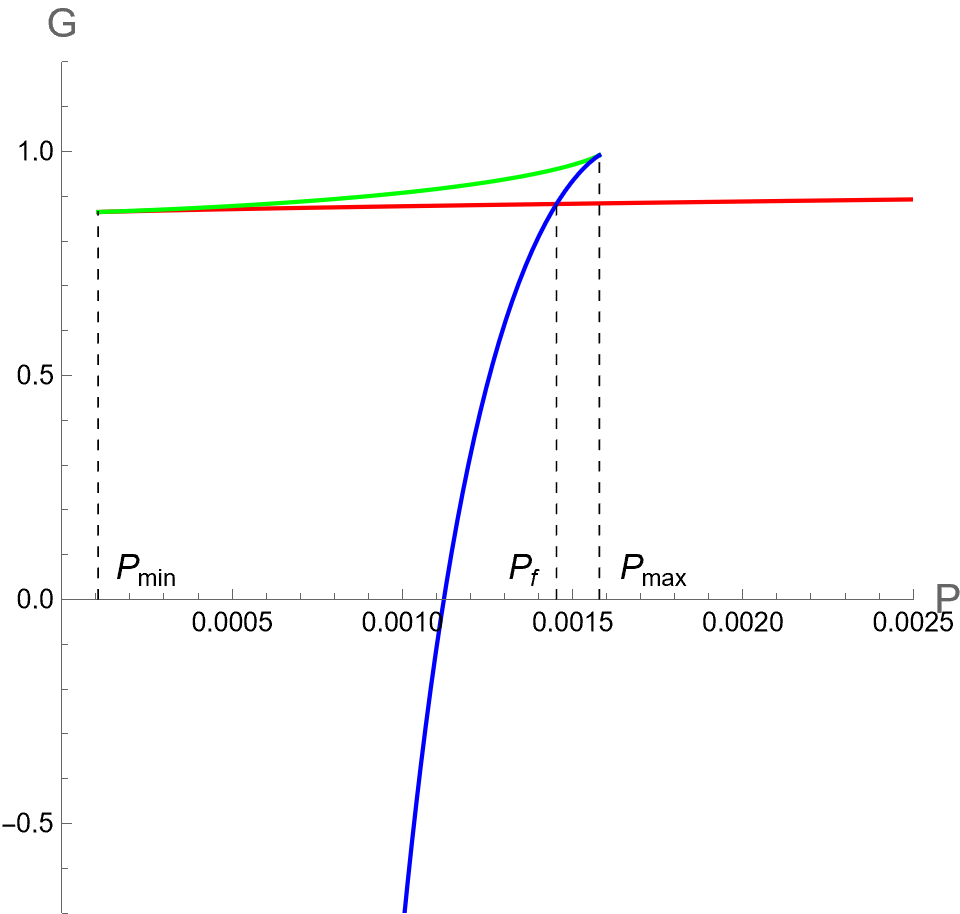
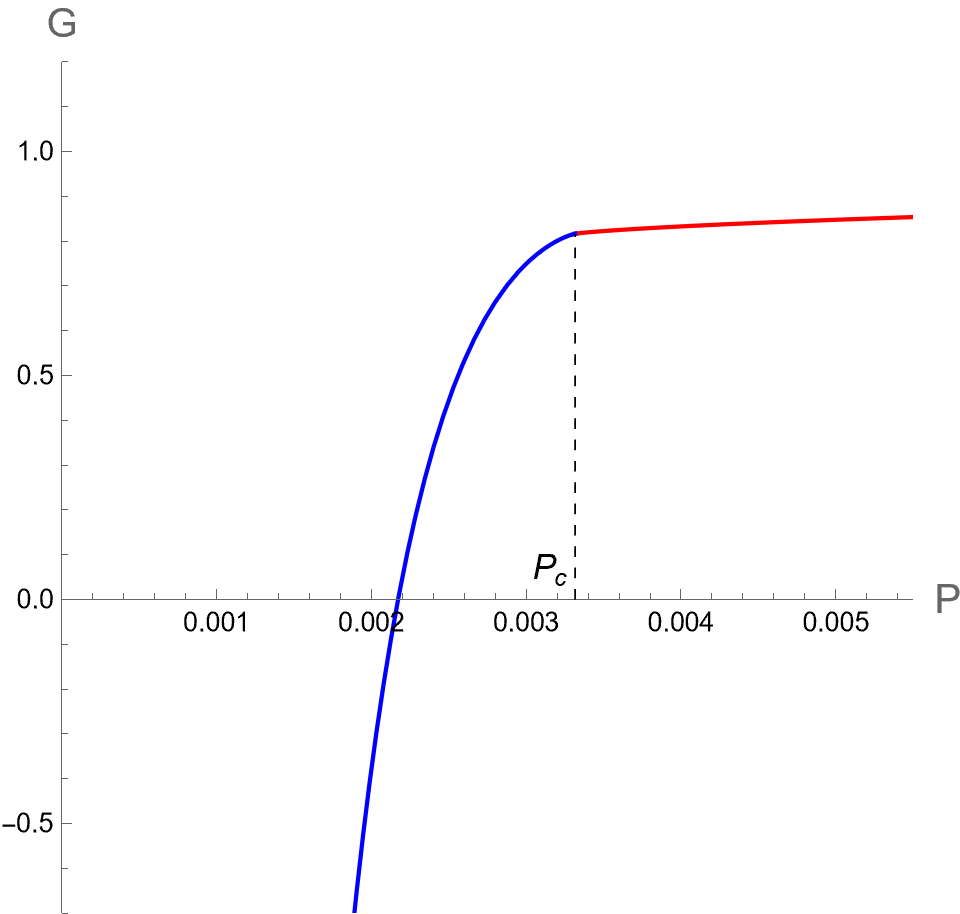
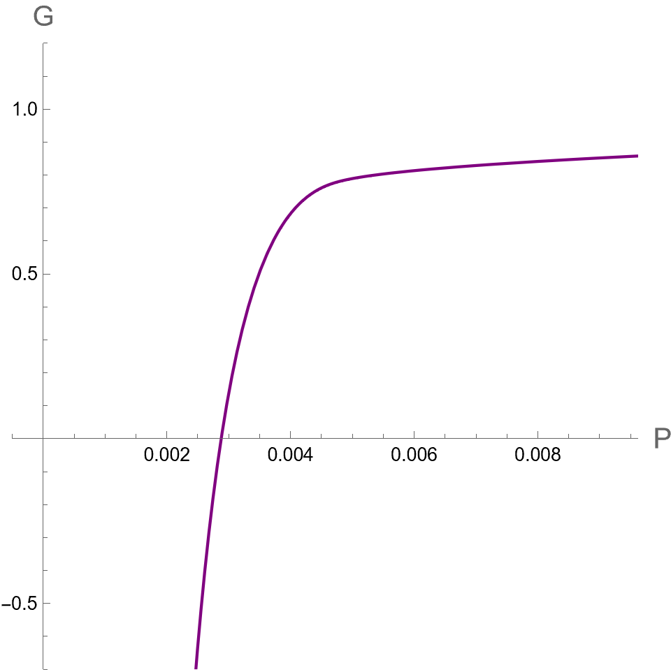
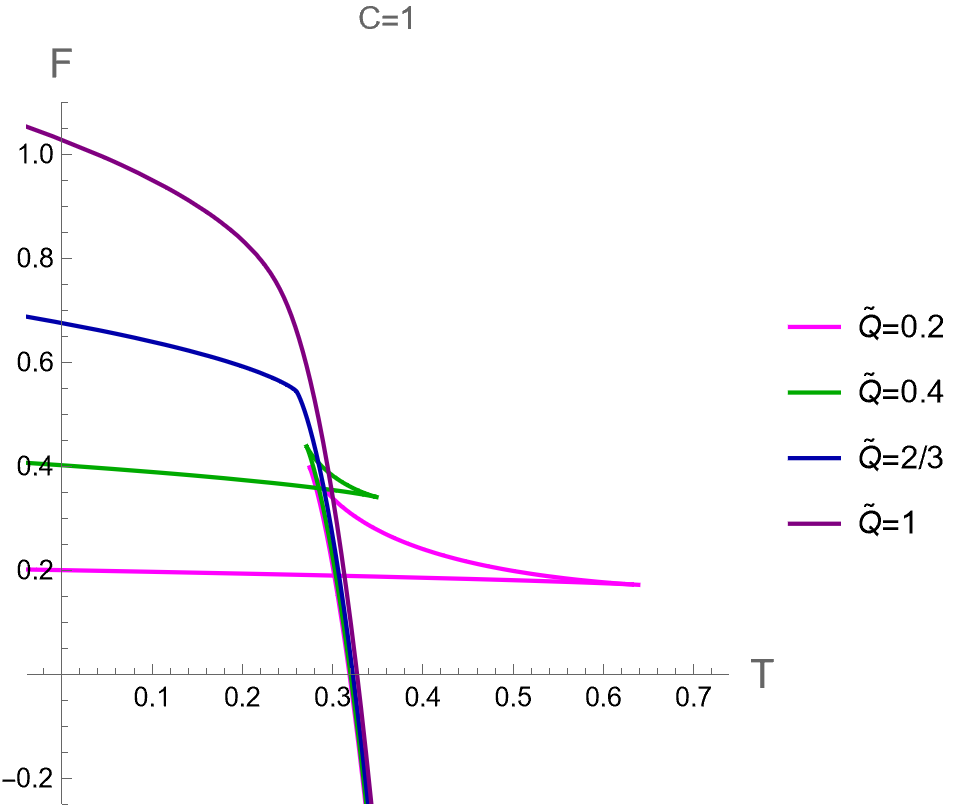
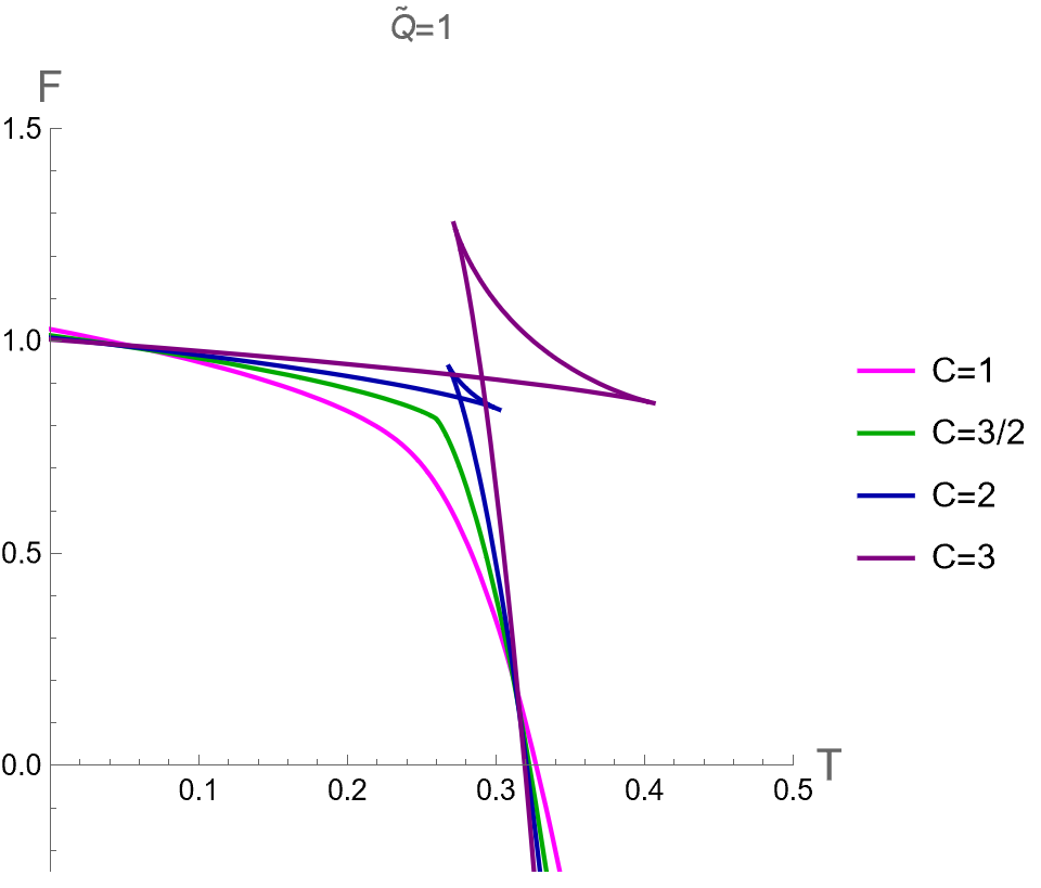
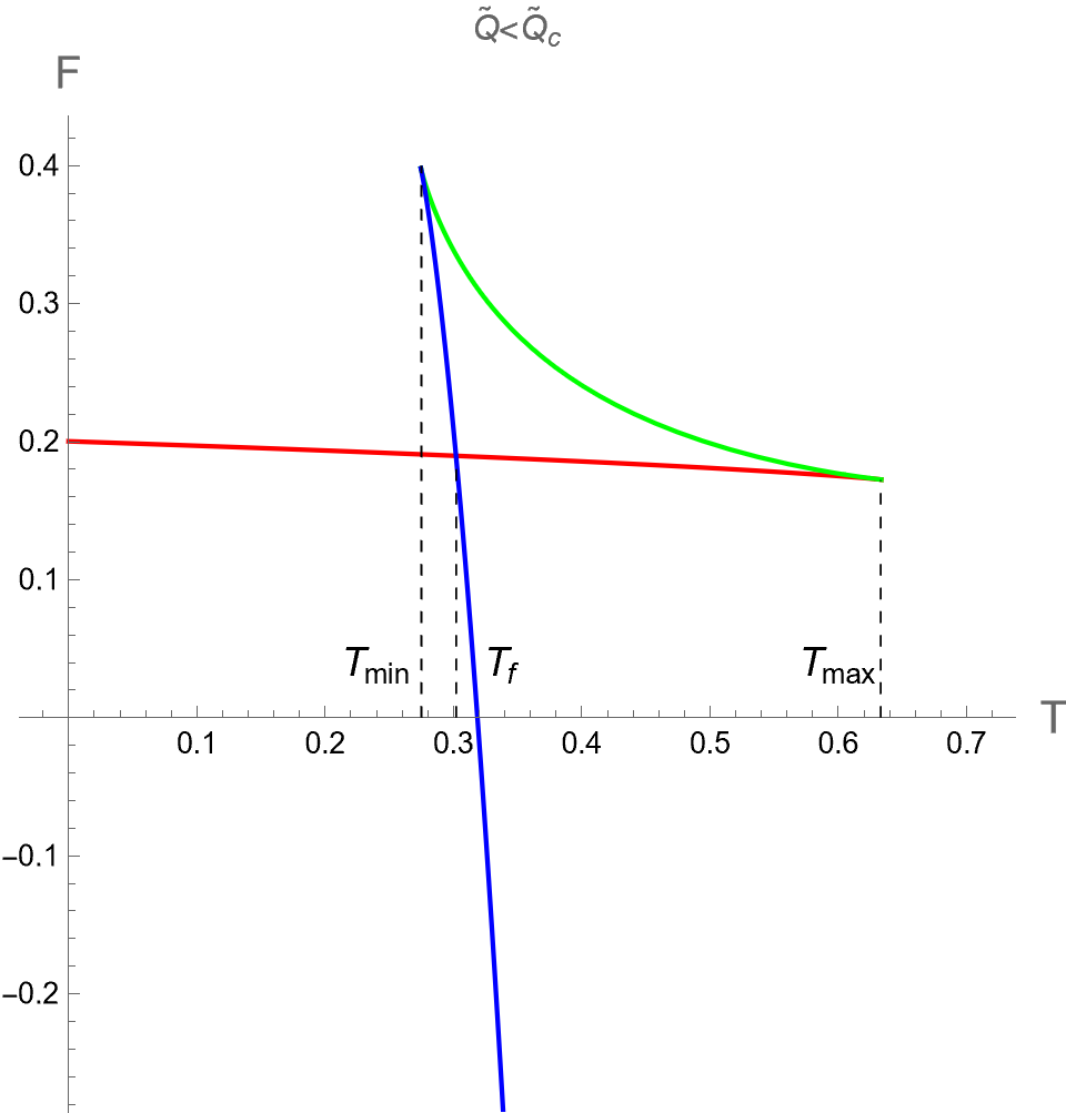
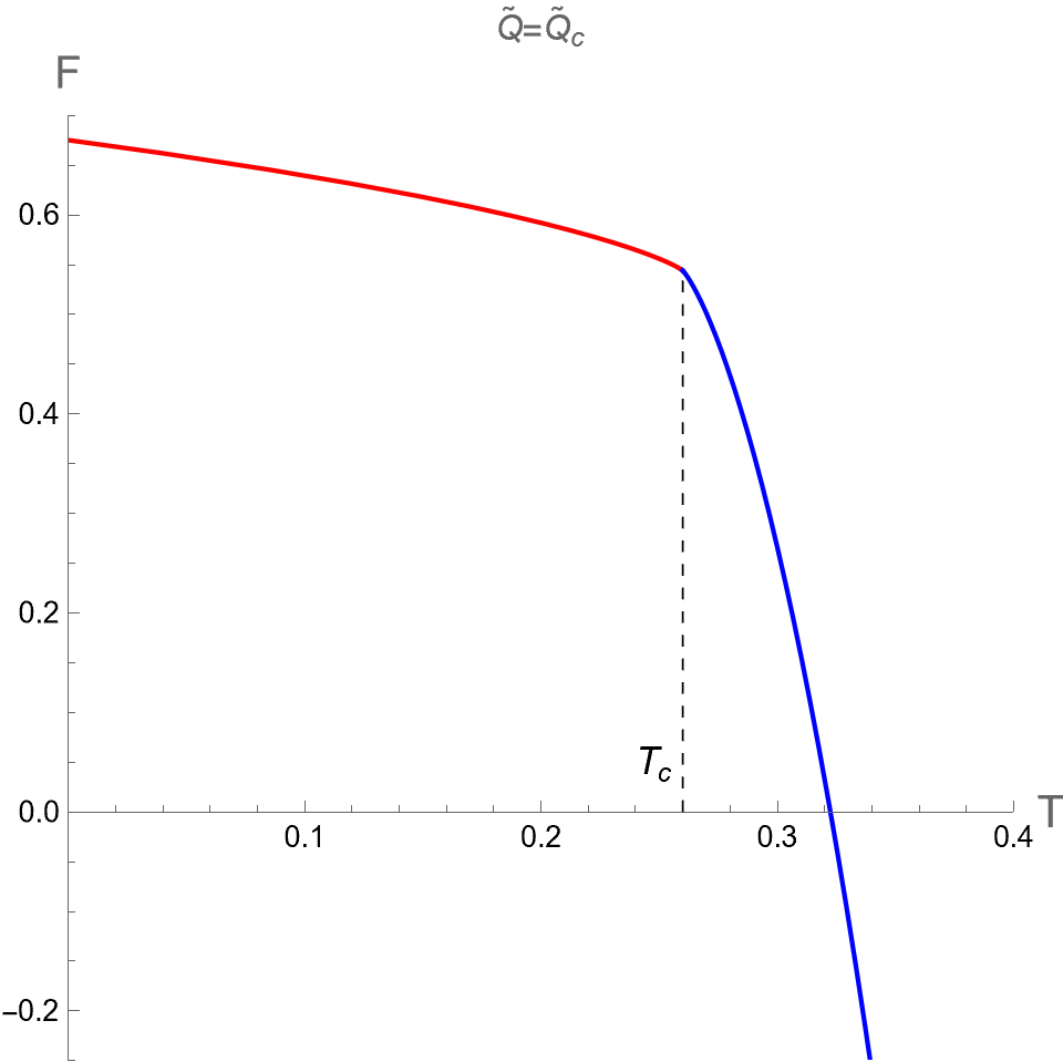
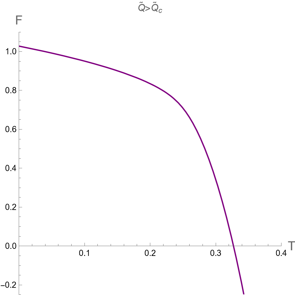
We plot against for a fixed in Fig. 2. It is important to note that the point where becomes divergent corresponds to a cusp in the graph. This feature reflects the second-order phase transition resulting from . As shown in the left panel in Fig. 2, the free energy in the case of , exhibits the swallowtail behavior with two cusps at and corresponding to the horizon radii that diverges and , respectively. Considering the bulk pressure running from a low value where only Large-BH exists, Small and Intermediate BHs both emerge at with free energy larger than the Large BH. Obviously, Large BH is thermodynamically preferred in the region of . It turns out that the system encounters the first-order phase transition at such that Small BH phase becomes thermodynamically preferred when . The middle panel in Fig. 2 shows the case of where the Small-Large BHs transition becomes the second-order type of phase transition at . The right panel in Fig. 2 shows that only one phase of BH exists at high temperature , here at , where at all values of . Remarkably, by identifying Small, Intermediate, and Large BHs as liquid, metastable, and gas phases, respectively, the behaviors of the BH phase transition is in a similar way as what occurs in the vdW fluid.
II.3 Holographic thermodynamics approach
As mentioned in section I, Introduction, the pressure and thermodynamic volume characterizing BHs in the bulk through the extended phase space approach do not directly correspond to the pressure and volume of the dual field theory on the boundary within the AdS/CFT correspondence. Additionally, the Smarr formula, which relates the mechanical quantities of BHs to thermodynamic variables, depends on the number of spacetime dimensions, this feature is typically absent in the Euler equation for ordinary matter. Recently, the holographic thermodynamics approach has provided insights into effectively addressing these two issues in associating the black hole thermodynamic properties with its dual field theory counterpart. In this section, we examine the thermodynamics of CFT, which is holographically dual to the charged AdS-BH, within the holographic thermodynamics approach.
Introducing the central charge and its chemical potential as a new pair of thermodynamic variable in the large- gauge theory, the author in [31] suggests that the scaling behavior of its internal energy may be written as
| (41) |
where denote the conserved quantities, such as charge and angular momentum. The Euler equation and its corresponding first law due to the Euler scaling argument can be obtained by using Eqs. (125) and (126) in Appendix A as
| (42) | |||||
| (43) |
where
| (44) |
Note that the term is absent in the Euler equation but the term appear in the first law. Since the variation of in Eq. (42) should be equal to the first law in Eq (43), i.e., , this implies the Gibbs-Duhem equation as follows
| (45) |
The grand potential is given by
| (46) | |||||
where we have substituted by using Eq. (42).
Since depends on both and due to the holographic dictionary as shown in Eq. (5), thus varying in the dual field theory should be equivalent to variation of and in the gravity side. By including and into the mass formula of AdS-BH in Eq. (127), an infinitesimal change of can be obtained from Eq. (126) as
| (47) |
where an additional partial derivative of with respect to is . Substituting in term of other variables by using the Smarr formula in Eq. (2) with expressed in term of , the above equation becomes
| (48) |
Thermodynamic variables of dual field theory can be identified with geometric quantities of AdS-BH as
| (49) |
Substituting them into Eq. (48) and comparing with Eq. (43), we obtain
| (50) |
where
| (51) |
Notably, the former relation in (51) expresses the pressure , in the field theory side, satisfies the equation of state in Eq. (4), while the latter gives the Euler equation corresponding to Eq.(42) with identifying and . It is interesting to note that the CFT in the field theory side from the approach of holographic thermodynamics can live in the curved spacetime with the curvature radius , which has a value not necessarily equal to the bulk AdS radius . This can be seen by redefining the thermodynamic variables as [31, 32]
| (52) |
From the resulting first law, we have and . Thus, the volume and central charge of the dual CFT are now independent due to the choice of rescaling as shown in Eq. (52).
It is worthwhile to review here some interesting results about the thermodynamics of CFT that are holographically dual to charged AdS-BH within the novel holographic thermodynamics approach. For simplicity, we define the dimensionless quantities:
| (53) |
The thermodynamic quantities of the dual CFT, which is in -dimensional spacetime of curvature radius , can be written in parametric equations of and as follows [32]
| (54) | |||||
| (55) | |||||
| (56) | |||||
| (57) | |||||
| (58) | |||||
| (59) |
Here, the field theory under consideration lives in the spacetime with dimensions. The CFT is in the ensemble with fixed , corresponding to the canonical ensemble. The temperature and heat capacity of the dual CFT are given by
| (60) | |||||
| (61) |
From Eq. (60), the horizon radius of extremal BH can be written as a function of and as
| (62) |
Due to the criticality of charged AdS-BH, thermodynamics of dual CFT also critically change in a similar way as the ratio crosses the critical point, which can be determined from the point of inflection as follows
| (63) |
Solving these two conditions, we obtain
| (64) |
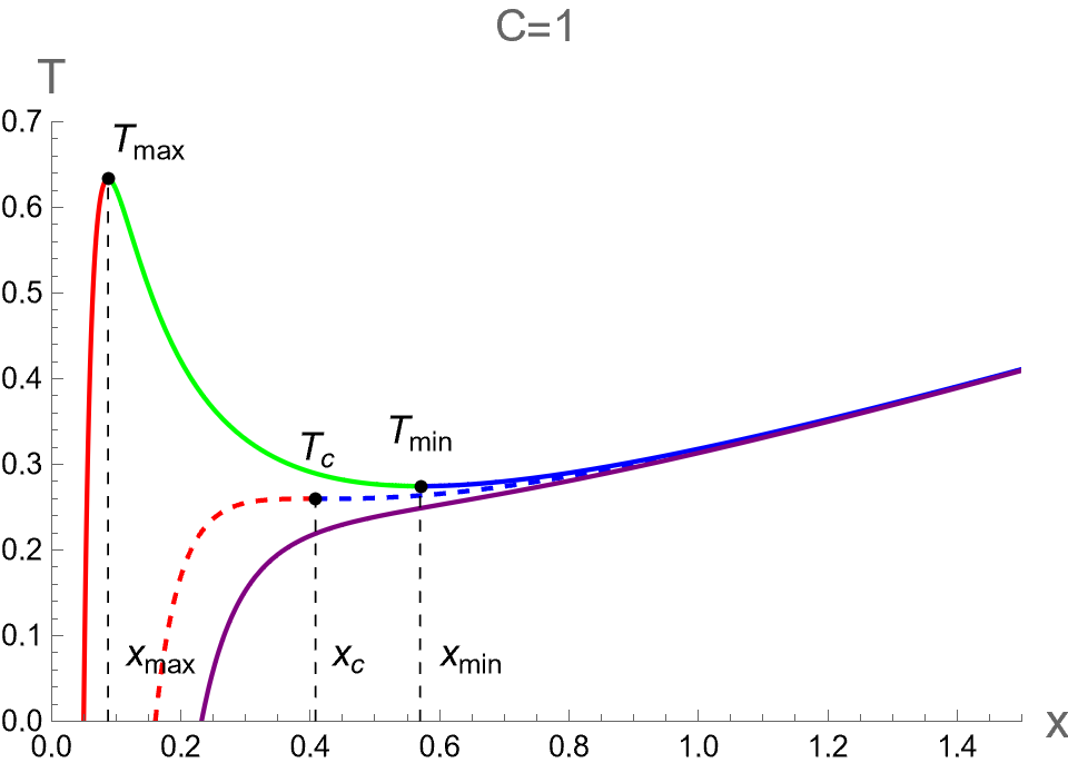
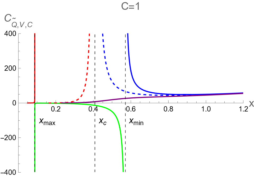
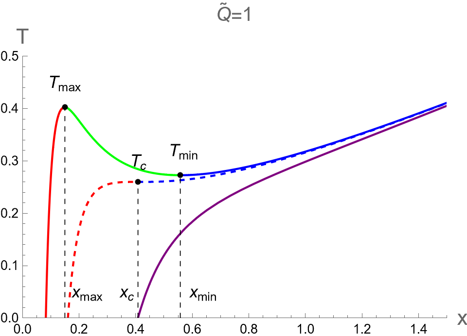
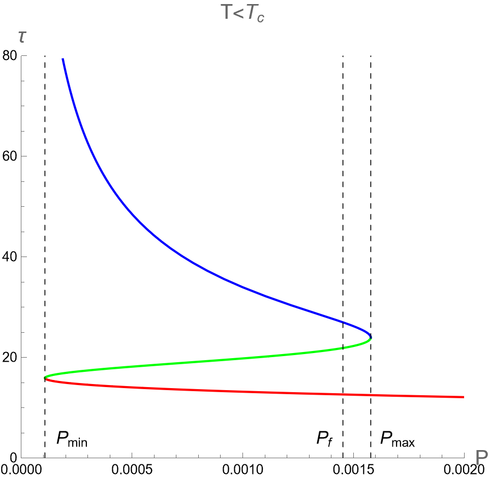
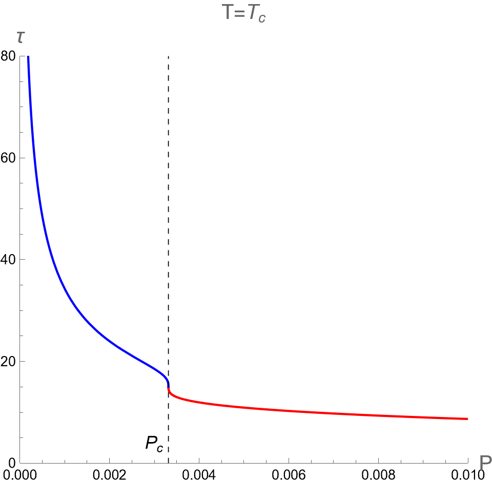
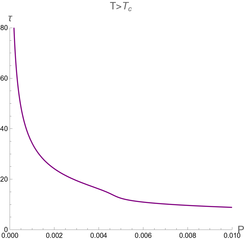
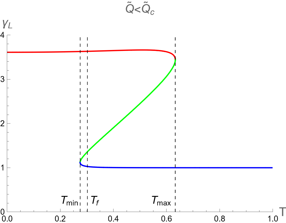
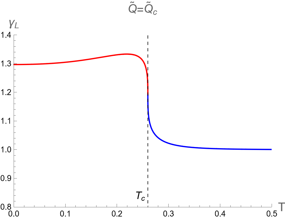
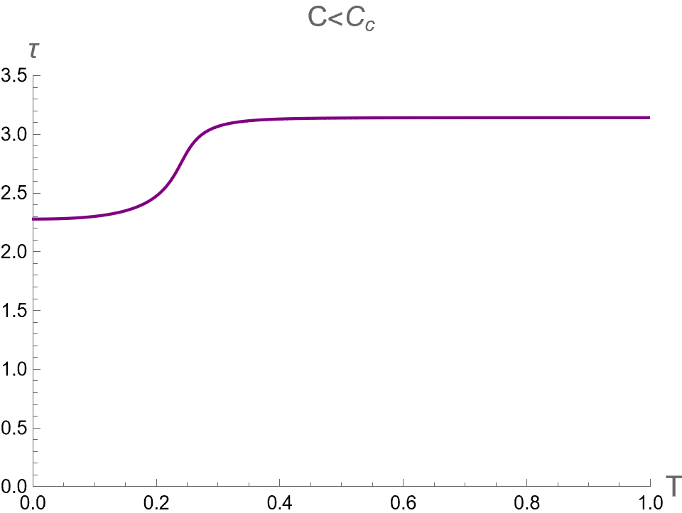
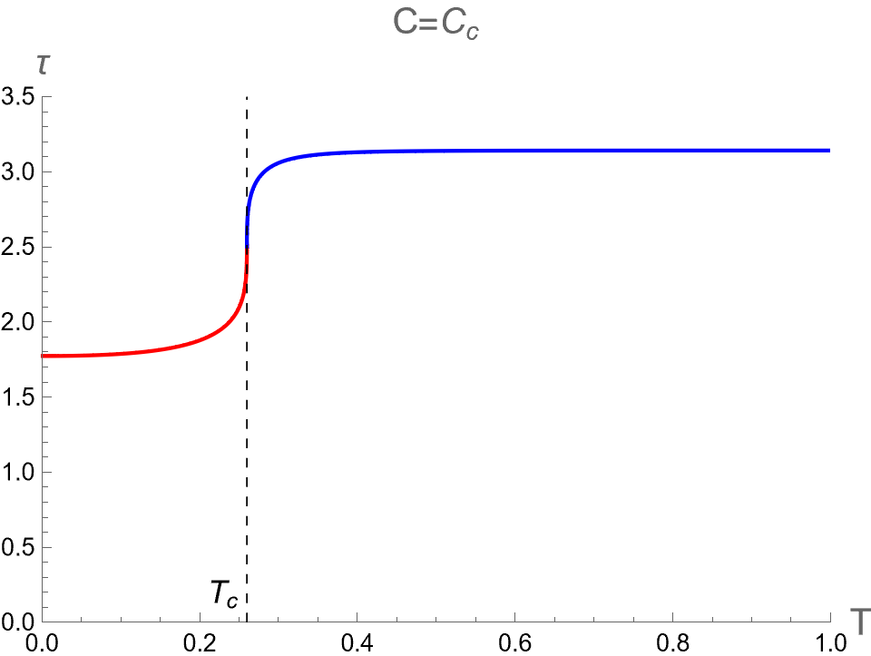
We examine thermal phase structures of dual CFT in two cases: (I) fixed with different values of and (II) fixed with different values of . We illustrate the behaviors of and as functions of for the former and latter cases in the first and second rows of Fig. 3, respectively. Note that and are given by
| (65) |
Two radii and indicate positions of local maximum and minimum of Hawking temperature as shown in Fig. 3 (a) and (c), namely and . At the critical value of , these two radii coincide at , which corresponds to the critical temperature . Remarkably, there exist three thermal states of dual CFT for in case (I) and in case (II). These three states consist of pCFT1 (red), nCFT (green), and pCFT2 (blue), which refers to the states of positive heat capacity when , negative heat capacity when , and positive heat capacity when , respectively. It is important to note that our notation might cause some confusion when is less than . As defined above, and in this paper refer to the points at which the temperature is at its maximum and minimum, respectively. Please do not be confused by these terms.
| Case I | Case II | |||||
|---|---|---|---|---|---|---|
| 0.0498 | 0.161 | 0.232 | 0.408 | 0.161 | 0.0825 | |
| 0.571 | - | - | - | - | 0.558 | |
| 0.0876 | - | - | - | - | 0.149 | |
| - | 0.408 | - | - | 0.408 | - | |
| 0.275 | - | - | - | - | 0.273 | |
| 0.633 | - | - | - | - | 0.403 | |
| - | 0.260 | - | - | 0.260 | - | |
| 0.302 | - | - | - | - | 0.291 | |
Using the Maxwell’s equal area law, the curve associated with the unstable nCFT phase in the plane in cases (I) and (II) can be replaced by a horizontal line, which indicates the first-order phase transition between these pCFT1 and pCFT2. In Appendix B, we elaborate on the detailed calculations using the method employed by [77] to obtain the Hawking-Page phase transition temperature within the holographic thermodynamics framework. The temperatures for cases I and II are as follows:
| (66) |
and
| (67) |
respectively, where and . The horizon radii for Small and Large BHs of case I and II are expressed respectively as follows
| (68) | |||
| (69) |
and
| (70) | |||
| (71) |
Note that we summarize our numerical results of some important parameters in our study in Table 1.
The thermodynamic potential associated with fixed ensemble is the Helmholtz free energy
| (72) |
The variation of reads
| (73) | |||||
where we have used Eq. (50) for , this yields
| (74) |
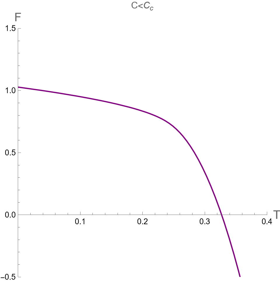
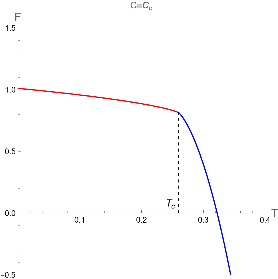
As pointed out in [32], there is no critical point found in the plane in the dual CFT. This result from the holographic thermodynamics is different from the criticality behavior from the extended phase space approach as discussed in last subsection. Therefore, we will consider as a function of instead of with constant or to investigate the global stability of dual CFT. By considering as a parameter, we parametrically plot between in Eq.(72) and in Eq.(55) for dual CFT in the case (I) and (II) as shown in the left and right panels of Fig 4, respectively. There are cusp points in curve where diverge. At these points, there are the second-order phase transitions occuring, manifested from the fact that , which can be derived via the first relation in Eq. (74).
We will discuss about the phase transition of dual CFT via its curve in more details as follows. First, let us consider in the case (I). We depicted the curves when , and in figures (a), (b) and (c) of Fig 5. The free energy shows the swallowtail shape for . In this case, the pCFT1 phase is thermodynamically preferred in low temperatures, i.e. both in the region of and . There is a first-order phase transition from pCFT1 to pCFT2 occurring at . At slightly higher than , the pCFT2 phase becomes the most thermodynamically preferred since it has the lowest free energy. The swallowtail shape of curve with shrink to appear as a kink at , where the transition between pCFT1 and pCFT2 phases become the second-order type of phase transition. For , there is only one phase with continuous curves with positive heat capacity for any , thus no phase transition occurs.
We plot versus in the case (II) in Fig 5 (d), (e) and (f) from small to large values of . The results indicate that phase structures of dual CFT in case (II) are qualitatively similar to the case (I). Namely, displays the swallowtail shape of three phases for , the pCFT1-pCFT2 first-order phase transition occurs at . At the critical value of , the nCFT disappears and the transition between pCFT1 and pCFT2 becomes the second-order phase transition at . For the small values of , there is only one thermal state of CFT with positive heat capacity at any value of .
III Critical Parameters in Photon Ring Region
The photon trajectories play a crucial role in determining the images of BH surrounded by emitting matter. Computing such null geodesics has become particularly interesting since the first image of a black hole was published by the Event Horizon Telescope Collaboration [41, *ETH2, *ETH3, *ETH4, *ETH5, *ETH6, *EventHorizonTelescope:2022wkp, *EventHorizonTelescope:2022apq, *EventHorizonTelescope:2022wok, *EventHorizonTelescope:2022exc, *EventHorizonTelescope:2022urf, *EventHorizonTelescope:2022xqj]. In this section, we will explore null geodesics in the spacetime of charged AdS black holes. This analysis aims to provide a clear understanding of three critical parameters in the photon ring region: the orbital half-period , the angular-Lyapunov exponent , and the temporal-Lyapunov exponent . These parameters play an important role in investigating black hole phase transitions through the BH’s optical characteristics.
The Lagrangian of test particle moving in the curved spacetime of the metric in Eq. (7) is given by
| (75) |
where denotes the affine parameter for a null geodesic. Since the spacetime is static and spherical symmetric, so the motion of test particle is confined in a plane that we can choose (equatorial plane) without loss of generality. The coordinates and are cyclic coordinates due to the symmetry of the background, resulting in the energy and angular momentum of test particles can take the form
| (76) |
where they are the constant of motion. The equation of motion in the radial direction reads
| (77) |
where the effective potential is given by
| (78) |
Note that and correspond to null-like and time-like geodesics, respectively. In the following formulas, we only consider the case of photon trajectories, i.e., . The unstable circular orbit can be determined by
| (79) |
where is the radius of unstable photon sphere. Using the first condition in (79) together with (77), we obtain
| (80) |
where denotes a critical impact parameter. Solving the second condition in Eq. (79), we obtain
| (81) | |||||
which is independent of angular momentum .
III.1 Orbital half-period
The incoming photons with impact parameter larger than and close to can wind several times around the BH before scattering back to the asymptotic region of spacetime. This effect can cause the light to take different paths around the BH, leading to the formation of multiple images of the source as seen by the distant observer.
Remarkably, the travel time before photons arrive at the observer screen along their null geodesics in different images is not generally equal because of the strong gravity caused by BH. This phenomenon is called the gravitational time delay, which could be measured via the gravitational lensing observation.
It is found that the time delay between successive images in the photon ring region is governed by the time-lapse over each half-orbit of a photon sphere [78, 79, 80]. The half-time period depends only on the metric spacetime. In other words, turns out to be independent of the distance of the light source from observers. This implies that is the parameter that is appropriate to encode the important feature about the region of spacetime near the event horizon.
To obtain the orbital half-period of the bound photon orbit, we can start by calculating the angular velocity of incoming photons measured by a distant observer. Using Eq. (76), we obtain
| (82) |
where we have used . At the photon sphere radius , the angular velocity is given by
| (83) |
Since the time lapse over a full orbit is , therefore the orbital half-period reads
| (84) |
III.2 Angular-Lyapunov exponent
As evident from the fact that and , the orbiting photons at are unstable. The Lyapunov exponents measure the sensitivity of the system to changes in initial conditions, which in this work refers to slight alterations in the photon trajectories near from one to a neighboring one. In this subsection and the following one, we investigate the sub-rings structure of photon trajectories in the region very close to the unstable photon sphere by using two Lyapunov exponents, namely the angular-Lyapunov exponent and temporal-Lyapunov exponent [81, 82]. Studying BH’s images of some given emitting light sources indicates that the ratio of photon flux received between adjacent sub-rings is determined by [67, 83, 82].
To obtain , we linearize Eq. (77) near the unstable shell of photon sphere in . The effective potential becomes . Consequently, one finds that
| (85) |
Expanding around and using two conditions in Eq. (79), we obtain
| (86) |
Applying the second relation of Eq. (76) into Eq. (86), which leads to the formula describing the angular dependence of the deviation from as follows:
| (87) |
where we have defined the angular Lyapunov exponent as
| (88) |
The angular dependence of the deviation is given by
| (89) |
where is the initial deviation of a geodesic from the critical circular orbit.
III.3 Temporal-Lyapunov exponent
Gravitational waves emitted by BHs during the ringdown phase are characterized by QNMs. However, determining the QNMs from the field perturbation of BH can be accomplished by examining the unstable circular geodesics of photons. Specifically, the temporal-Lyapunov exponent is related to the imaginary part of the complex quasinormal frequency. Namely, we have as the timescale for the instability of the ringdown amplitude. Consequently, associated with the photon ring region serves as an important parameter for studying BHs under various scenarios.
We calculate , which represents the deviation rate in time of photon trajectory from the unstable photon sphere. With the first relation of Eq. (76), we obtain the rate from Eq. (86) as follows:
| (90) |
where we have defined the temporal-Lyapunov exponent
| (91) |
Thus, the time evolution of is
| (92) |
where is the initial deviation of a geodesic from the photon sphere.
IV Probing Black Hole Phase Transitions through Optical Features
In this section, we will investigate BHs undergoing thermal phase transitions by exploring three critical parameters involving the optical features of BHs introduced in the previous section. As discussed in the Introduction, section I, it is worthwhile to investigate thermal phase transitions through optical probing in the extended phase space approach and holographic thermodynamics. As will be shown later in this section, the results from both approaches indicate that these parameters, treated as functions of either or , can express discontinuities as well as behaviors of multi-valued functions. This is in a similar way to exploring thermodynamic phase transitions of conventional substances by observing abrupt changes in their free energy and response functions as or are varied. For convenience, we use where to represent the three critical parameters: , , and represent , , and , respectively. These three critical parameters can potentially serve as order parameters in the consideration of phase transitions, as we will discuss later in Section V.
IV.1 Probing the phase transition in the extended phase space approach
The thermal profiles of in the extended phase space can be considered as a function of either or separately, i.e., or . This is because in Eq. (81) can be written as and as follows:
| (93) | |||||
| (94) |
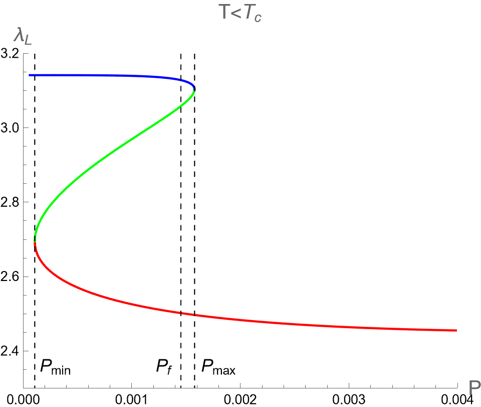
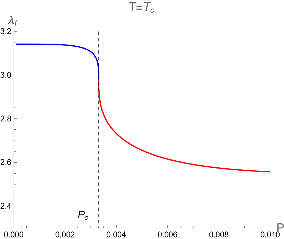
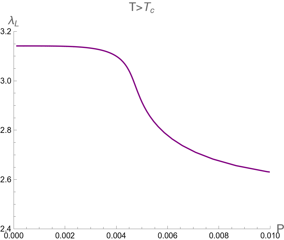
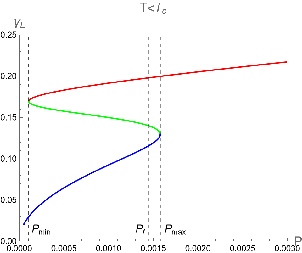
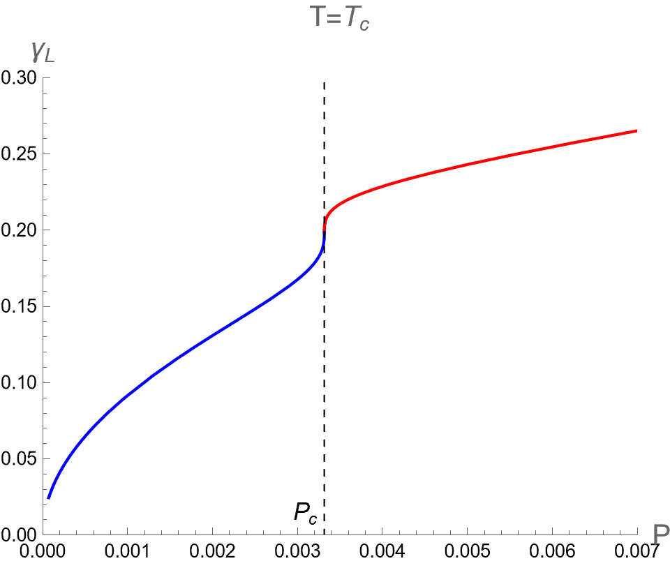
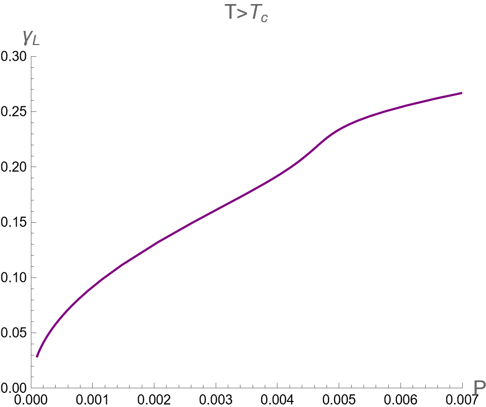
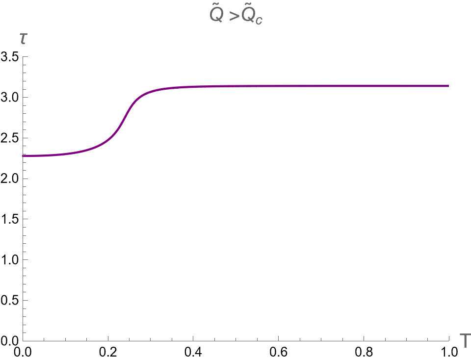
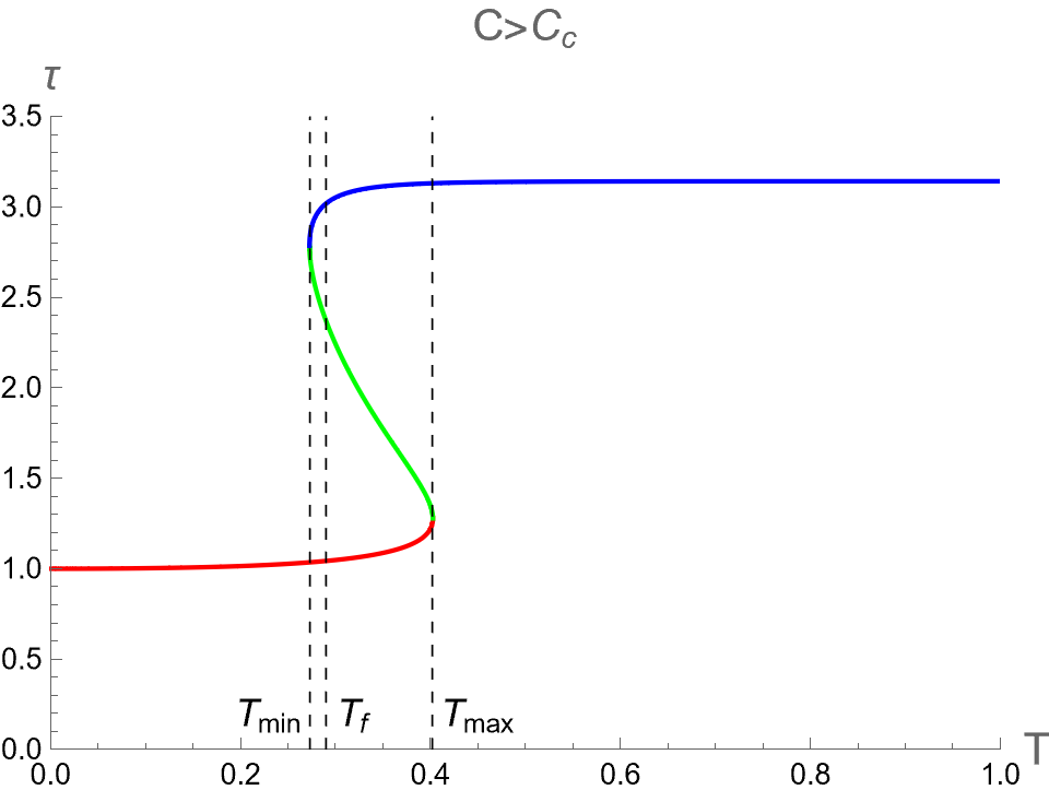
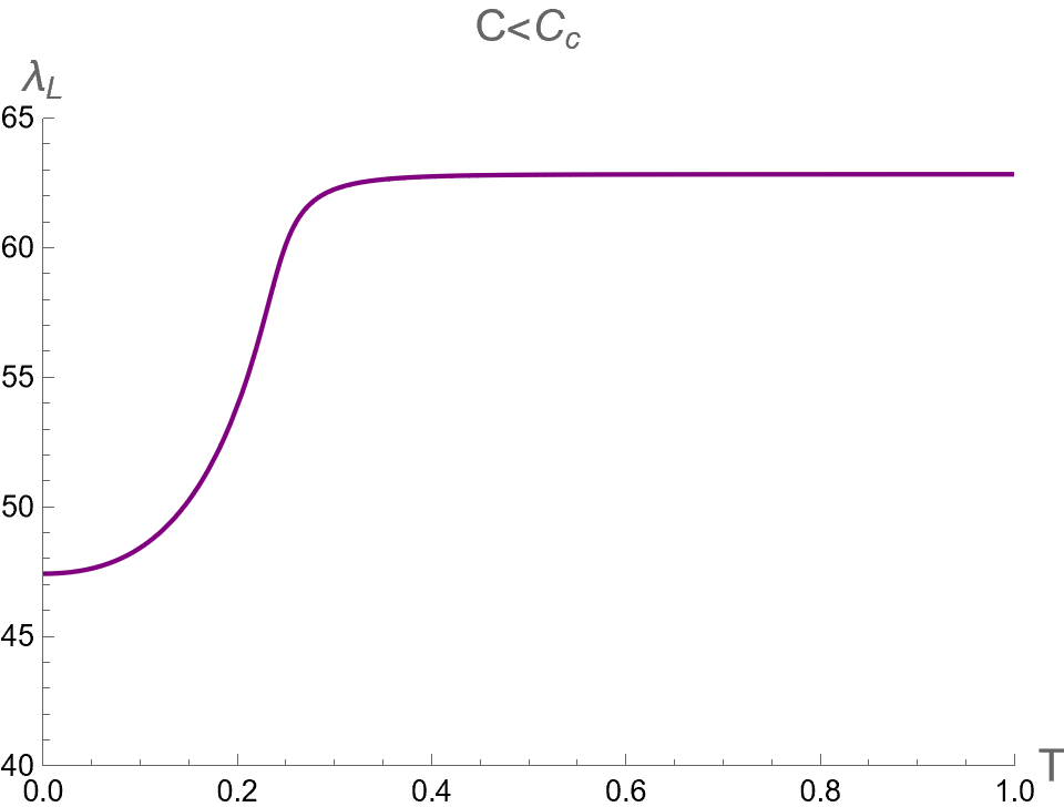
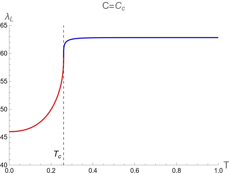
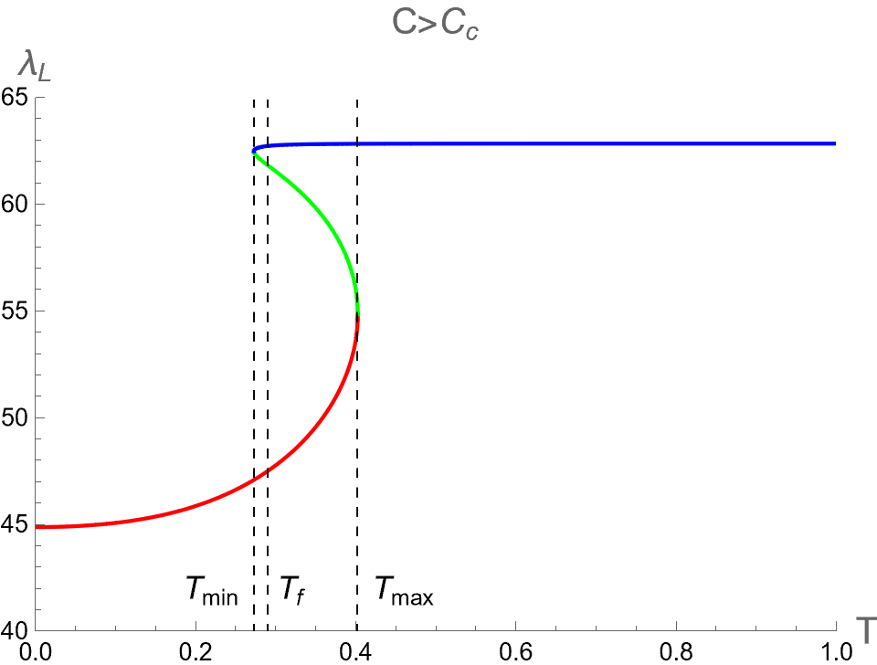
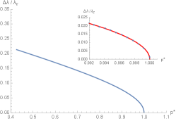
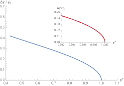
In the context of the extended phase space, the present paper focuses on the effect of on three critical parameters during BH phase transitions in the isothermal process. Namely, we analyze the discontinuities and multi-value behavior of as functions of while keeping constant. By substituting as described in Eq. (94) into Eqs. (84), (88) and (91), one can use as a parameter running in the parametric plot as the isotherm curves, i.e. versus the bulk pressure . Note that the bulk pressure has been described in Eq. (28). The isotherm curves of and , as a function of , are illustrated in the first, second and third rows of Fig. 6, respectively. The left, middle and right columns of Fig. 6 depict the cases with and , respectively.
When , the three critical parameters exhibit a multi-value function within the range , as shown in the left column of Fig. 6. In other words, at the values of in this range, there are three values for each corresponding with the Small (red), Intermediate (green) and Large-BHs (blue) branches. Outside this range of pressure, there exists only one branch, namely the Large-BH branch for and the Small-BH branch for . Interestingly, the isotherm curves of three critical parameters at expressed itself as a multi-value function has the boundary at and , which correspond to the positions of the cusps of (see Fig. 2) with the divergent value of (see Fig. 1). Therefore, considering the parameters can exhibit the second-order phase transition of charged AdS-BH from observing the divergence of their derivative with respect to . Remarkably, when a Small-Large BHs first-order phase transition occurs at , the values of will discontinuously change between Small and Large BH branches due to discontinuity jumping of event horizon radius caused by the Maxwell equal area law. This is an important result that will be applied in our study about the criticality, as discussed in the next section.
As the temperature is larger, the pressures and converge and degenerate to be at , namely the Intermediate-BH phase becomes absent, as shown in the middle colums of Fig. 6. The values of three critical parameters at the critical point of the second-order phase transition between Small (red) and Large (blue) BHs can be expressed as follows
| (95) |
Note that we use . For is larger than , it turns out that only one BH solution exists and no phase transition occurs.
IV.2 Probing the phase transition in holographic thermodynamics
In this subsection, we probe phase structures of charged AdS-BH in the holographic thermodynamics approach via three critical parameters, i.e. , and . The expression for the photon sphere radius in Eq. (81) can be written in term of the bulk parameters and , as defined in Eq. (53), in the form
| (96) |
To investigate the influence of and of the boundary CFT on the behaviors of null geodesics around critical photon orbits in bulk spacetime, can be substituted using Eq. (57) into the above equation in terms of and as following
| (97) |
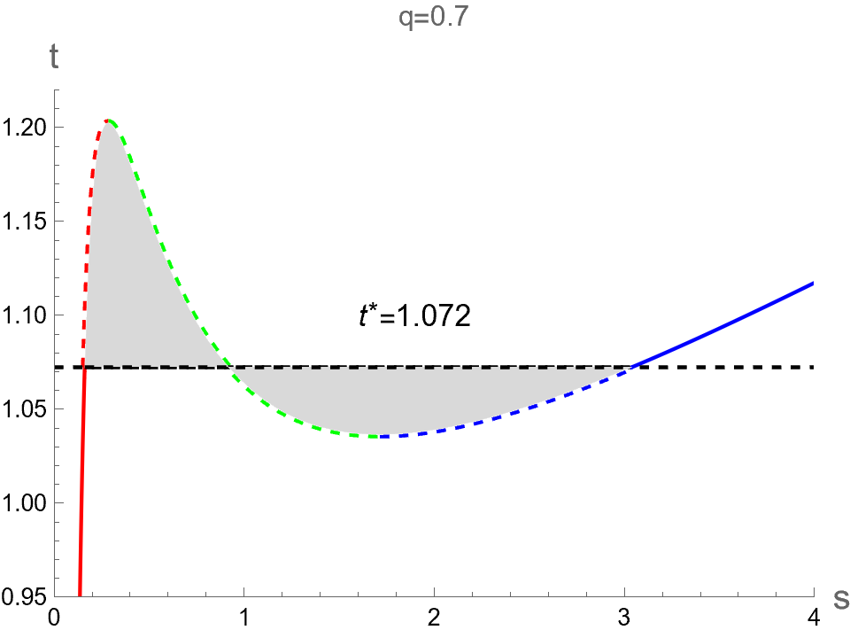
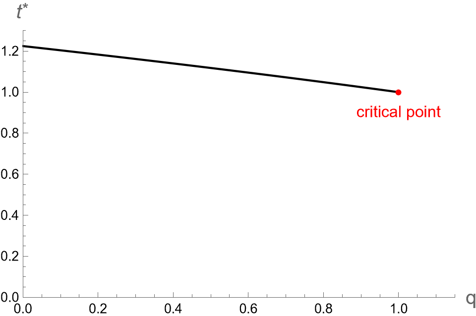
Since the criticality is absent in the boundary thermodynamics and no term appears in the Smarr formula, we focus on the behavior of as a function of instead for the holographic thermodynamics. Substituting into Eqs. (84), (88) and (91), one can express , and versus for study the influence of and on in the case I and case II as discussed before, respectively.
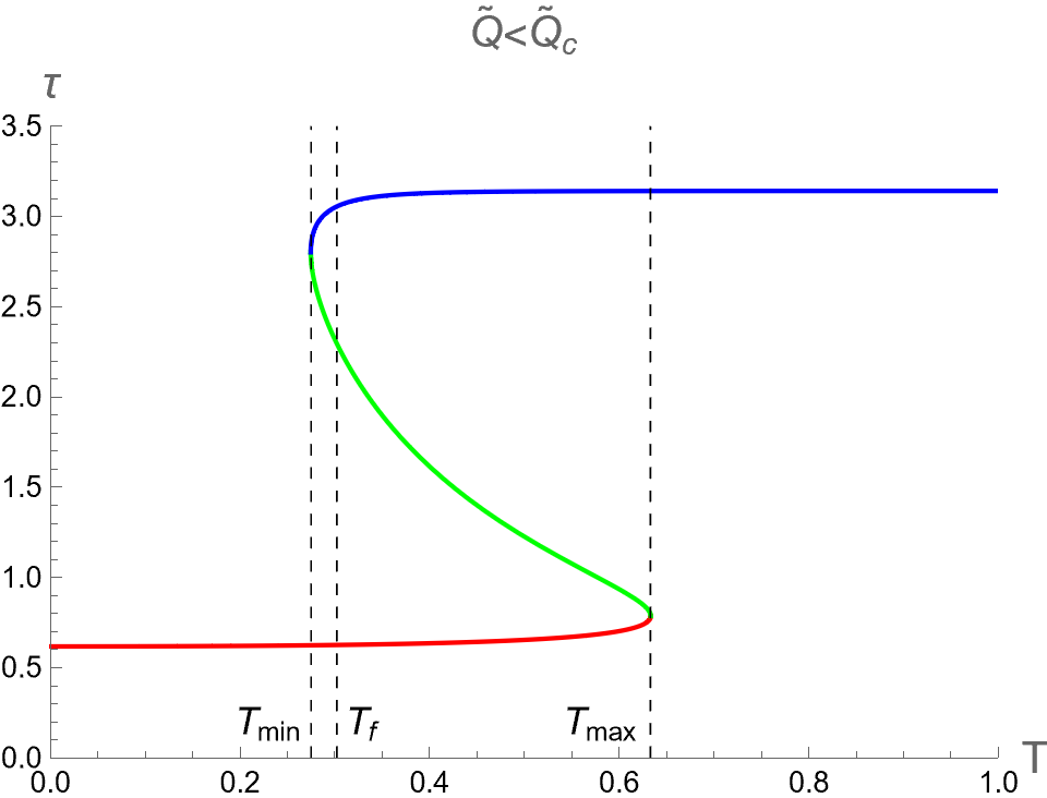
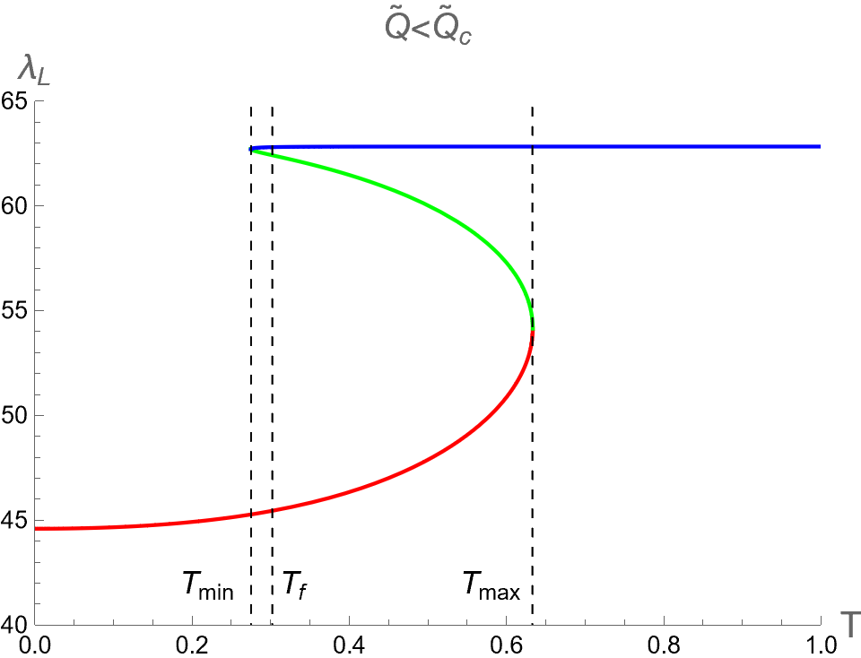

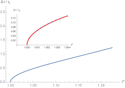
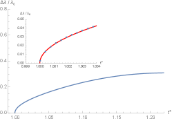
In the case I, the behaviors of versus for , and are illustrated in the left, middle and right columns in Fig. 7, respectively. From the graph of with for dual CFT (see the figure (a) of Fig 5) reveals that three phases of CFT, namely pCFT1, nCFT and pCFT2 coexist when implying that the Small, Intermediate and Large-BH phases also coexist in this range of in the gravity picture. We find that the parameters associated with the critical curve in exhibits a multi-value function, i.e. three phases of BH have three different values of , as shown in the left column in Fig. 7. Outside this range of , there exists only one phase, namely the Small-BH phase for and the Large-BH phase for . Moreover, the slope of isocharge curves in the plane diverges at and , which correspond to the positions of cusp of with the divergent of . Remarkably, when pCFT1-pCFT2 first-order phase transition occur at , the values of will discontinuously change between Small-BH and Large-BH phases due to discontinuos jumping of entropy. This can be exhibited by the Maxwell equal area law as illustrated in Appendix B. This remarkable results from the present study could reveal the behaviors of criticality, as will be discussed later in the next section.
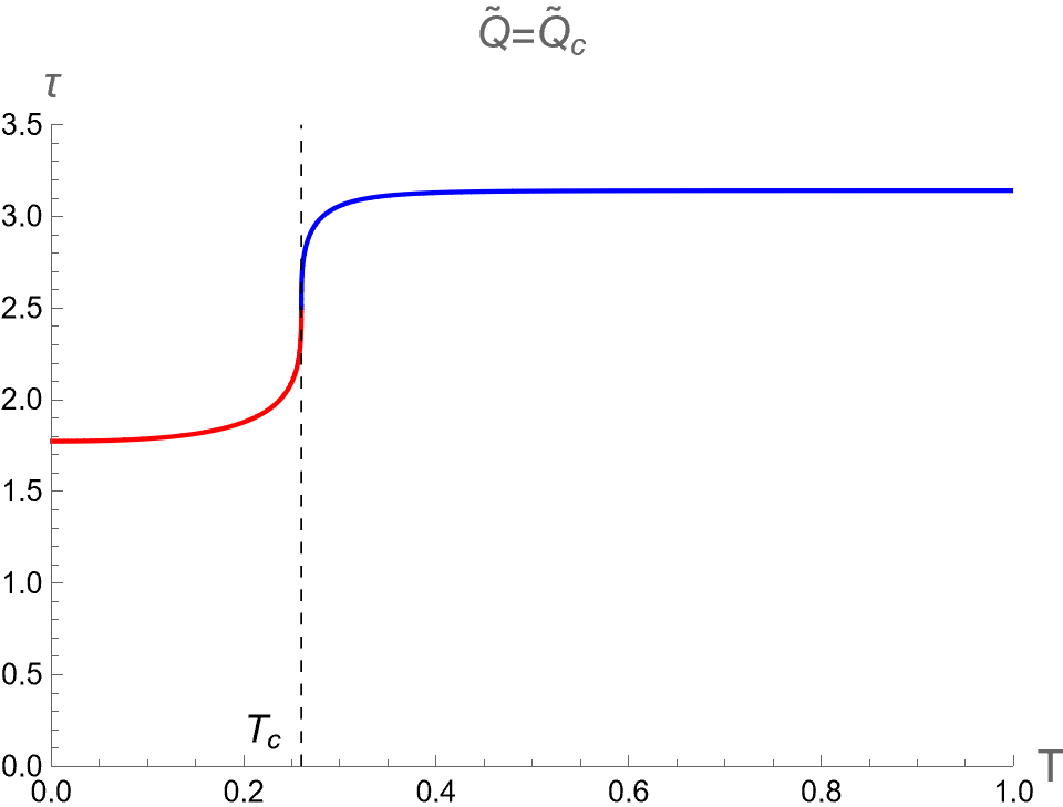
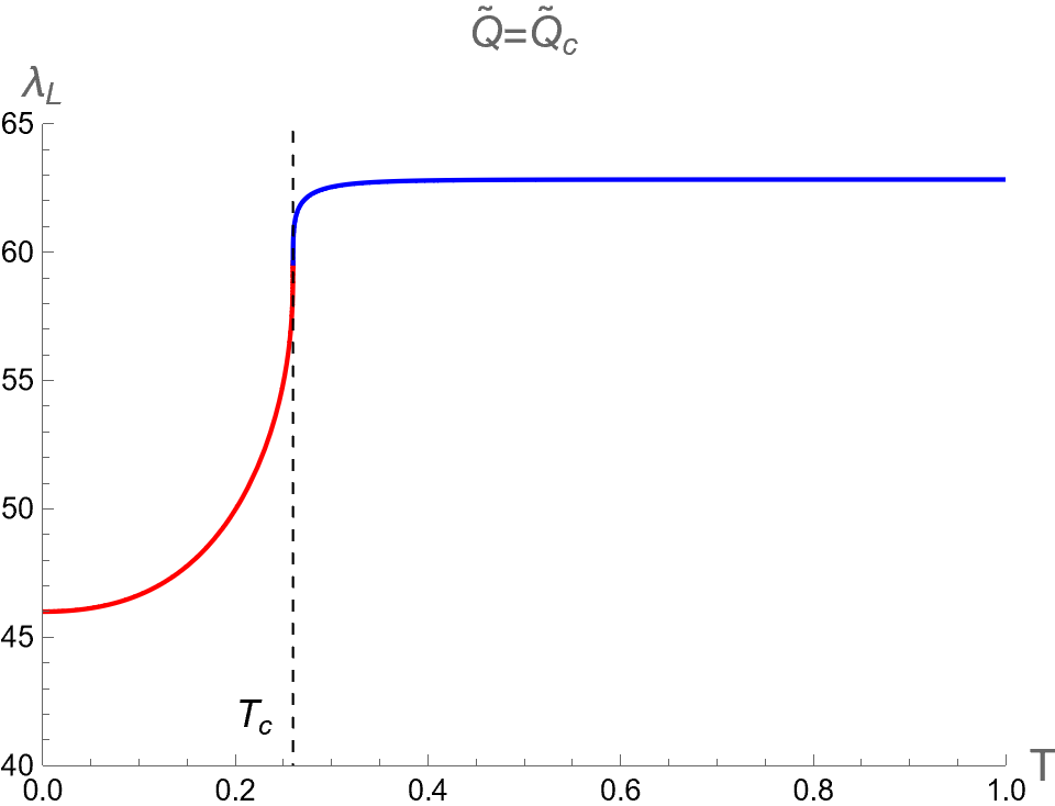
The middle column in Fig. 7 illustrates the case of . Notably, becomes a single-valued function, and Intermediate-BH phase disappears. Two distinct configuration of BHs, i.e. Small and Large-BHs, exist without coexistence. Furthermore, Small-Large BHs second-order phase transition takes place at , where the critical values of , and can be expressed as follows:
| (98) |
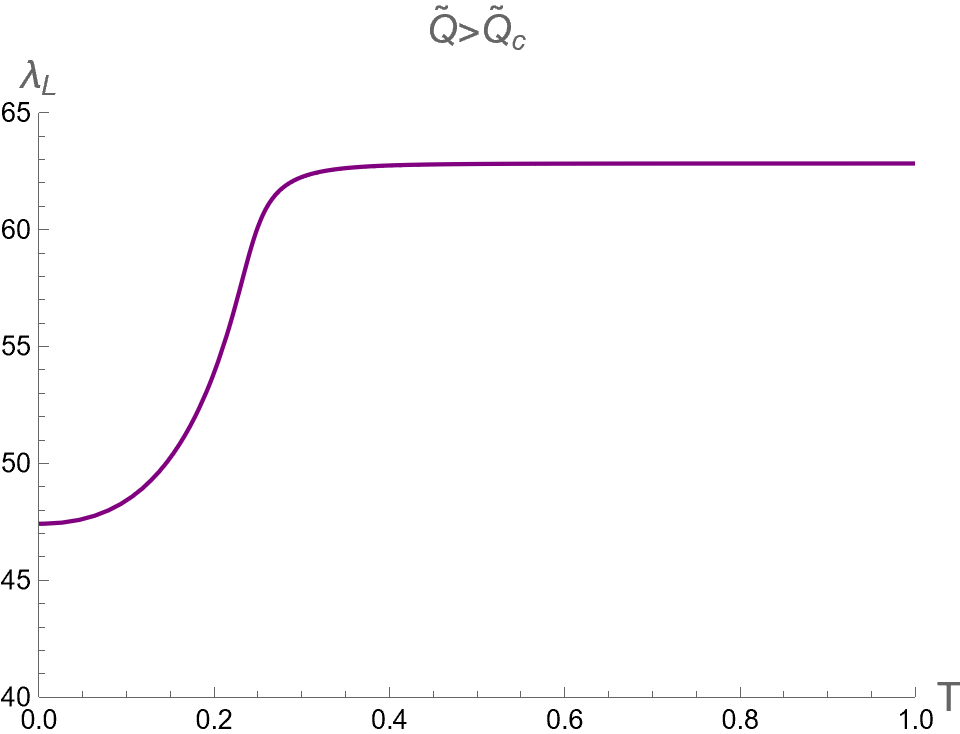
In the right column of Fig. 7, we examine the scenario where . In this case, the BH is characterized by a single phase (purple curve).
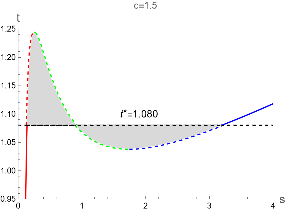
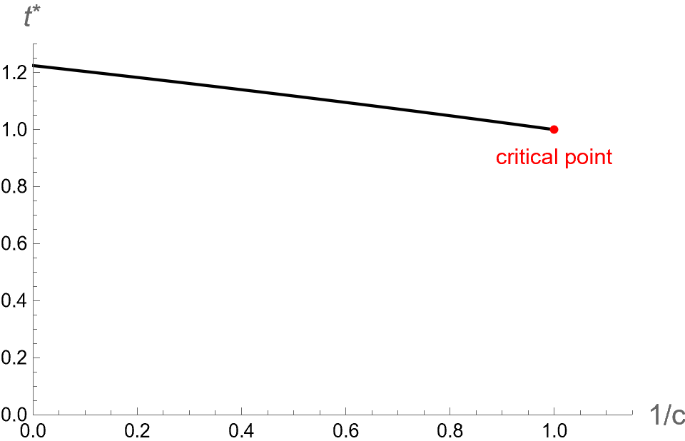
By introducing as a new thermodynamic variable, we investigate its influence on in the case II as shown in Fig. 8. We examine the curves of versus in scenario in the left column in Fig. 8. Since the BH and its dual CFT on the boundary exist in a single phase without any phase transition, the curves exhibit no multi-value function and discontinuity.
In the case of , the curves display a single-value function, whose derivative with respect to diverges at . The BH configurations below and above the critical temperature correspond to the Small and Large BH phases, respectively. Note that the values of , and at the critical point of case II is the same as those of case I, as shown in Eq.(98).
For , we find that the parameters in range exhibits a multi-value function. Namely, three different values of correspond to three phases of BH, as shown in the right column in Fig. 8. Outside this range of , there exists only one phase, namely the Small-BH phase for and the Large-BH phase for . Moreover, the slope of constant- curves in the plane diverges at and , which correspond to the positions of cusp of with the divergent value of .
V Scaling Behavior of the optical parameters
In this section, we investigate the scaling behavior of the BH’s optical appearance parameters . In phase transition studies, scaling behavior typically emerges near the critical transition point, where different types of matter can exhibit similar scaling laws for thermodynamic quantities. The scaling behavior with identical critical exponents across different types of matter suggests that these matters belong to the same universality class, independent of their particle composition and interactions. Notably, the critical exponents in the scaling law are crucial for understanding the nature of matter near the critical point of phase transition.
To investigate the system near the critical point, we focus on order parameter that vanishes at this point, while maintaining non-zero values prior to reaching it. In examining the dependence of , , and on and within the extended phase space approach and holographic thermodynamics, there is a potential that can serve as an order parameter, where subscripts and denote Small and Large BHs, respectively. At and , where the Small-Large BH phase transition occurs, experiences a discontinuous jump, indicating . As the value of or changes along the phase boundary, the values of for Small and Large BHs become increasingly similar, causing to decrease, eventually reaching zero at the critical point.
Here, we will categorize the phase transition of the charged AdS-BH in the extended phase space and holographic thermodynamics description via investigating the scaling law of . In particular, our analysis in this section will show that the scaling law can be written in the following form
| (99) |
in the extended phase space approach, whereas in the form
| (100) |
in holographic thermodynamics approach. Note that denotes the value of at the critical point. Moreover, and are the proportionality constants, and are the critical exponents. Recall that and , as previously defined in section II.
V.1 Extended phase space approach
Let us consider the system near the critical point, one can apply the power series expansion to express and as follows
| (101) | |||
| (102) |
where and are the horizon radii of Small and Large BHs at Hawking-Page pressure. The order parameter is then
| (103) |
From Eq. (35) and (36), the leading order of and around the critical point is given by
where
| (104) |
Thus
| (105) |
Expanding the reduced Hawking-Page pressure as expressed in Eq. (34) near the critical temperature , we obtain
| (106) |
It is important to emphasize that we are considering the system near the critical point, allowing us to express the above equation up to the first order of , thereby neglecting higher-order terms. Consequently, we can use this first-order approximation to eliminate in Eq. (105). By substituting the result into Eq. (103), we obtain
| (107) |
where could be expressed as
| (108) |
From Eq. (107), we observe that the critical exponent , which suggests that its behaviors are in the same way as the vdW fluid type. The scaling behavior for three optical order parameters are
| (109) | |||||
| (110) | |||||
| (111) |
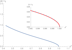
Using Eqs. (34), (35), (36) and (94), we can determine each pair of the reduced order parameters and the reduced Hawking-Page pressure by running the temperature increasing from the minimum value to . Recall that we have shown the formula of in Eq. (31). In other words, by writing in the form of reduced temperature , we run from to the critical value , and then we obtain the plot of the reduced order parameters versus , as shown in Fig 9. Notably, we find that three reduced order parameters decrease as increase and become vanish at . In the zoomed panels, the blue points represent the numerical values of the exact results of the reduced order parameter near the critical point.
Interestingly, the expressions of the scaling laws, as shown in Eqs. (109), (110) and (111), provide the results that fit the blue points remarkably well, as illustrated as the red curves. These indicate that the three order parameters exhibit a discontinuous jump, resulting in non-vanishing within the range . This behavior signifies the occurrence of a second-order phase transition at . At this critical point, all order parameters vanish as and converge to the same value. Beyond the critical point, the order parameters no longer exhibit multiple values, indicating the presence of a single BH phase.
V.2 Holographic thermodynamics approach
In the case of the holographic thermodynamics approach, we consider the power series expansion of around the critical point up to the first order as
| (112) | |||
| (113) |
where and refer to the horizon radii for Small and Large BHs at the first-order phase transition, respectively. The reduced order parameters near the critical point are then
| (114) |
Let us consider the phase transition in the case I first. As is fixed while can be varied, we define the parameter as
| (115) |
The expression of and in Eqs. (68) and (69) can be expanded around as follows
By keeping up to only the leading order, the difference between these two horizon radii is given by
| (116) |
Since we consider the behavior of reduced order parameters whose values are calculated at the Hawking-Page temperature near the critical temperature , let us write , Eq. (66), in the form of the series expansion as
Keeping up to only the leading order, we can have
| (117) |
Consequently, using Eqs. (116) and (117), Eqs. (114) can be rewritten in the form of the scaling law of reduced order parameters as
| (118) |
where the proportionality coefficient is
| (119) |
As obviously shown in Eq. (118), the critical exponents of three order parameters for and .

For the case II of phase transition in the holographic thermodynamics approach, we introduce
| (120) |
According to the previous approximation, we find that the scaling law for three reduced order parameters near the critical point of case II is the same as case I as follows
| (121) | |||||
| (122) | |||||
| (123) |
Since the scaling behavior near the critical point of reduced order parameters in case II is similar to case I, we will display the plot of three reduced order parameters versus the reduced Hawking-Page temperature only in case I, as illustrated in Fig 10. Using Eqs. (66), (68), (69) and (97), can be determined at fixed versus , with running from 1 to 0 in case I, whereas it is determined at fixed versus with running from 1 to in case II. On the other hand, the figure indicates that three reduced order parameters are more than zero starting at and terminating at , beyond which a Hawking-Page phase transition does not exist. This can also be seen from Fig. 11 (b) in Appendix B. In the zoomed panels, the blue points represent the numerical values of the exact results of the reduced order parameter near the critical point. Interestingly, the expressions of the scaling laws, as shown in Eqs. (121), (122) and (123), provide the results that fit the blue points very well, as illustrated as the red curves. These indicate that the three order parameters exhibit a discontinuous jump, resulting in non-vanishing within the range . This behavior signifies the occurrence of a second-order phase transition at . At this critical point, all order parameters vanish as and converge to the same value. For , the order parameters no longer exhibit multiple values, indicating the presence of a single BH phase.
It is worth emphasizing that in the extended phase space approach, the scaling law can be found near the critical point for these three optical order parameters as a function of , where all exhibit the critical exponent with the value of . On the other hand, in holographic thermodynamics where the concepts of bulk pressure and volume are absent, the scaling law behavior can also be found near the critical point for these parameters as a function of with the critical exponent equal to . The results in the holographic thermodynamics context are particularly noteworthy because they do not rely on bulk pressure and volume. This suggests that the critical behavior of BHs can be understood only in terms of boundary field theory quantities.
VI Conclusions
In this study, we have thoroughly examined the intricate phase structures of charged AdS-BHs within the extended phase space and holographic thermodynamics approaches by analyzing null geodesics near their critical curves. By utilizing horizon-scale observation of BHs, namely the orbital half-period , angular Lyapunov exponent , and temporal Lyapunov exponent , we can characterize BH phase transitions in these two frameworks.
In particular, for the extended phase space approach, when , these three critical parameters are multi-valued functions of bulk pressure , indicating the presence of three coexisting phases of BH. When , these parameters display the singled-valued function versus corresponding with a single BH phase.
In the holographic thermodynamics approach, the phase transition of charged AdS-BH in the bulk is holographically dual to the CFT phase transition in the boundary with including the central charge and its conjugate as a new pair of thermodynamic variable. We investigate the phase structures of BH dual to the fixed ensemble of CFT. For or , the three critical parameters exhibit a multi-valued function of temperature , indicating the presence of three coexisting BH phases. Conversely, for or , these parameters display a single-valued function with respect to , corresponding to a single BH phase.
In many fields, including condensed matter physics, there are numerous examples of phase transitions that often lack a clearly defined order parameter or the concept may not be entirely appropriate. In this study, we propose the possibility of an order parameter based on the difference between each optical parameter of the Small and that of Large BH phases at the Hawking-Page phase transition. This approach is advantageous because upcoming space-based VLBI missions aim at studying the photon subring structure of BH, thereby providing a practical and observable method to characterize BH phase transitions. Remarkably, the critical exponents for these parameters near the critical point, from both extended phase space and holographic thermodynamics approaches, are found to be 1/2, indicating a significant thermodynamic similarity to van der Waals fluids. It is important to emphasize that, in our work, the scaling law near the critical point can be derived through precise theoretical calculations, avoiding any ambiguous methods.
Evidently, the BH optical appearance parameters from both approached are effective in characterizing BH phase transitions in AdS space. It is important to highlight that these critical parameters may be linked to some phenomena in strongly coupled systems through holographic duality. In the context of the AdS/CFT correspondence, a thermal state in the CFT is dual to a BH in the bulk AdS space. A perturbation in the dual field theory, induced by a local operator, corresponds to a perturbation of the BH by turning on the scalar fields propagating in the bulk. The process of returning to thermal equilibrium in the field theory side can be dual to the black hole returning to equilibrium after a perturbation, which can be observed through imaginary part of quasinormal frequencies describing the rate at which a perturbed BH returns to equilibrium. Consequently, the QNM spectrum of a BH can be interpreted holographically as the quantum Ruelle resonances in boundary theory, which are complex frequency modes that describe the late-time decay of perturbations in chaotic systems [84]. Moreover, in the eikonal limit, the decay of QNMs can be governed by the temporal Lyapunov exponent of unstable null geodesics [81, 85, 86, 87]. In this eikonal regime in the AdS-BHs background, there exist the long-lived modes, which dominate the late-time behavior of BH while returning to equilibrium [88, 89]. The existence of long-lived QNMs in AdS suggests that certain perturbations in the dual CFT decay very slowly, implying that the system takes a long time to return to thermal equilibrium. In our results, we find that at the Small-Large BHs phase transitions, the behavior of and hence the late-time behavior of long-lived modes change discontinuously due to the Maxwell equal area law. Holographically, this behavior presumably reflects a sudden change in the spectrum of Ruelle resonances across the first-order phase transition on the field theory side. The order parameter we propose could be valuable for extending studies on holographic thermalization in a field theory, particularly concerning phase transitions, in future research.
In particular, we focus on optically probing the phase structures of charged BH in AdS space, as they exhibit rich phase structures and undergo intriguing phase transitions, such as the Hawking-Page phase transition and critical behavior. However, it is also worthwhile to consider applying these methods to study BH phase transitions in more realistic scenarios, such as BHs in asymptotically flat or de Sitter (dS) spacetimes. Additionally, this approach could be extended to investigate BH phase transitions in the context of modified entropies [90, *Promsiri:2020jga, *ElMoumni:2022chi, *Tannukij:2020njz, *Nakarachinda:2021jxd, *Barzi:2024bbj, *MEJRHIT201945, *barrow2020area, *Jawad:2022bmi], providing a broader framework for understanding BH thermodynamics across different theoretical models.
Acknowledgement
EH is supported by Thailand Science Research and Innovation (TSRI) Basic Research Fund: Fiscal year 2023 under project number FRB660073/0164. WH is supported by the National Science and Technology Development Agency under the Junior Science Talent Project (JSTP) scholarship, grant number SCA-CO-2565-16992-TH. This research has received funding support from the NSRF via the Program Management Unit for Human Resources & Institutional Development, Research and Innovation [grant number B13F660066].
Appendix A Eulerian scaling argument
In the following discussions, we review how the first law of thermodynamics is obtained from the Smarr formula by using Euler’s theorem for a homogeneous function as detailed in [15, 16].
A function is a homogeneous function of degree if
| (124) |
The Euler’s theorem states that if is a homogeneous function of degree , then it satisfy the partial differential equation:
| (125) |
then an infinitesimal change of is given by
| (126) |
It is noticed that the mass of non-rotating charged AdS-BH can be expressed in terms of the area , the electric charge and the cosmological constant as follows
| (127) |
which is indeed the homogeneous function degree because . From Eq. (125), we have
| (128) |
Using Eq. (127), the partial derivative terms in the above equation can be derived as
| (129) |
and the Smarr formula is then
| (130) |
The formula in Eq. (126) give the variation of as follow
| (131) |
Identifying respectively, and its conjugate variable as the bulk pressure and volume via the relation in Eq. (3) in Eqs. (130) and (131), we will obtain Eqs. (25) and (26).
Appendix B Holographic Maxwell’s equal area law in plane
Here, we consider the calculations of pCFT1-pCFT2 phase transition temperature for CFT, which dual to the Small-Large BHs phase transition of charged AdS-BH in the holographic description. Substituting the horizon radius into Eq. (60) and then writing in the form of the entropy using the area law, we obtain as follows
| (132) |
We can define the reduced parameters as follows:
| (133) |
Consider case I as introduced in section II, we can express the reduced BH temperature in Eq. (132) in terms of and as
| (134) |
Interestingly, it does not explicitly depend on central charge . As shown in Fig. 11 (a), the reduced Hawking-Page phase transition temperature is represented in dashed-black horizontal line. This line is positioned such that the areas above and below the isocharge curve are equal, in accordance with Maxwell’s equal area law. With and representing the reduced entropy associated with pCFT1 and pCFT2 at the , respectively, the equal area law is expressed as
| (135) |
Then, we obtain
| (136) |
Note that the first-order phase transition appear when (). Substituting and into Eq. (134) together with Eq. (136), we obtain the system of equations as follows
| (137) | |||||
| (138) | |||||
| (139) |
These equations can be solved analytically by following the procedure as suggested in [77]. First, using the fact the RHS of Eq. (137) equal to Eq. (138), we obtain
| (140) |
where . Then, using , we have
| (141) |
By eliminating term via the relation in Eq. (140), we have the quartic equation in variable as follows
| (142) |
The nontrivial solution is . To obtain and , we substitute into Eq. (140) and solve following equations
| (143) | |||||
| (144) |
simultaneously. Since , therefore the solutions for and are
| (145) | |||||
| (146) |
Thus, becomes
| (147) |
For case II, we express the BH temperature in Eq. (132) by substituting and . The resulting does not depend on electric charge as following
| (148) |
Note that the first-order phase transition appears when (). Since Eqs. (134) and (148) is symmetric under , the solutions of variables and as a function of in this case can be written as follows
| (149) | |||||
| (150) | |||||
| (151) |
References
- Bekenstein [1973] J. D. Bekenstein, Black holes and entropy, Phys. Rev. D 7, 2333 (1973).
- Hawking [1975] S. W. Hawking, Particle Creation by Black Holes, Commun. Math. Phys. 43, 199 (1975), [Erratum: Commun.Math.Phys. 46, 206 (1976)].
- Bardeen et al. [1973] J. M. Bardeen, B. Carter, and S. W. Hawking, The Four laws of black hole mechanics, Commun. Math. Phys. 31, 161 (1973).
- Maldacena [1998] J. M. Maldacena, The Large N limit of superconformal field theories and supergravity, Adv. Theor. Math. Phys. 2, 231 (1998), arXiv:hep-th/9711200 .
- Witten [1998a] E. Witten, Anti-de Sitter space and holography, Adv. Theor. Math. Phys. 2, 253 (1998a), arXiv:hep-th/9802150 .
- Witten [1998b] E. Witten, Anti-de Sitter space, thermal phase transition, and confinement in gauge theories, Adv. Theor. Math. Phys. 2, 505 (1998b), arXiv:hep-th/9803131 .
- Gubser et al. [1998] S. S. Gubser, I. R. Klebanov, and A. M. Polyakov, Gauge theory correlators from noncritical string theory, Phys. Lett. B 428, 105 (1998), arXiv:hep-th/9802109 .
- Hawking and Page [1983] S. W. Hawking and D. N. Page, Thermodynamics of Black Holes in anti-De Sitter Space, Commun. Math. Phys. 87, 577 (1983).
- Smarr [1973] L. Smarr, Mass formula for kerr black holes, Phys. Rev. Lett. 30, 71 (1973).
- Jacobson and Visser [2019] T. Jacobson and M. Visser, Gravitational Thermodynamics of Causal Diamonds in (A)dS, SciPost Phys. 7, 079 (2019), arXiv:1812.01596 [hep-th] .
- Kastor et al. [2009] D. Kastor, S. Ray, and J. Traschen, Enthalpy and the Mechanics of AdS Black Holes, Class. Quant. Grav. 26, 195011 (2009), arXiv:0904.2765 [hep-th] .
- Dolan [2011a] B. P. Dolan, Pressure and volume in the first law of black hole thermodynamics, Class. Quant. Grav. 28, 235017 (2011a), arXiv:1106.6260 [gr-qc] .
- Dolan [2011b] B. P. Dolan, The cosmological constant and the black hole equation of state, Class. Quant. Grav. 28, 125020 (2011b), arXiv:1008.5023 [gr-qc] .
- Cvetic et al. [2011] M. Cvetic, G. W. Gibbons, D. Kubiznak, and C. N. Pope, Black Hole Enthalpy and an Entropy Inequality for the Thermodynamic Volume, Phys. Rev. D 84, 024037 (2011), arXiv:1012.2888 [hep-th] .
- Kubiznak et al. [2017] D. Kubiznak, R. B. Mann, and M. Teo, Black hole chemistry: thermodynamics with lambda, Classical and Quantum Gravity 34, 063001 (2017).
- Altamirano et al. [2014] N. Altamirano, D. Kubizňák, R. B. Mann, and Z. Sherkatghanad, Thermodynamics of Rotating Black Holes and Black Rings: Phase Transitions and Thermodynamic Volume, Galaxies 2, 89 (2014), arXiv:1401.2586 [hep-th] .
- Kubiznak and Mann [2015] D. Kubiznak and R. B. Mann, Black hole chemistry, Can. J. Phys. 93, 999 (2015), arXiv:1404.2126 [gr-qc] .
- Kubizňák and Mann [2012] D. Kubizňák and R. B. Mann, P- v criticality of charged ads black holes, Journal of High Energy Physics 2012, 1 (2012).
- Xu et al. [2015] J. Xu, L.-M. Cao, and Y.-P. Hu, P-V criticality in the extended phase space of black holes in massive gravity, Phys. Rev. D 91, 124033 (2015), arXiv:1506.03578 [gr-qc] .
- Majhi and Samanta [2017] B. R. Majhi and S. Samanta, P-V criticality of AdS black holes in a general framework, Physics Letters B 773, 203 (2017), arXiv:1609.06224 [gr-qc] .
- Altamirano et al. [2013] N. Altamirano, D. Kubizňák, and R. B. Mann, Reentrant phase transitions in rotating anti-de Sitter black holes, Phys. Rev. D 88, 101502 (2013), arXiv:1306.5756 [hep-th] .
- Gunasekaran et al. [2012] S. Gunasekaran, D. Kubizňák, and R. B. Mann, Extended phase space thermodynamics for charged and rotating black holes and Born-Infeld vacuum polarization, Journal of High Energy Physics 2012, 110 (2012), arXiv:1208.6251 [hep-th] .
- Wei and Liu [2015] S.-W. Wei and Y.-X. Liu, Insight into the microscopic structure of an ads black hole from a thermodynamical phase transition, Phys. Rev. Lett. 115, 111302 (2015).
- Wei et al. [2019] S.-W. Wei, Y.-X. Liu, and R. B. Mann, Repulsive Interactions and Universal Properties of Charged Anti-de Sitter Black Hole Microstructures, Phys. Rev. Lett. 123, 071103 (2019), arXiv:1906.10840 [gr-qc] .
- Wei et al. [2019] S.-W. Wei, Y.-X. Liu, and R. B. Mann, Ruppeiner Geometry, Phase Transitions, and the Microstructure of Charged AdS Black Holes, Phys. Rev. D 100, 124033 (2019), arXiv:1909.03887 [gr-qc] .
- Johnson [2014] C. V. Johnson, Holographic heat engines, Classical and Quantum Gravity 31, 205002 (2014).
- Dolan [2014] B. P. Dolan, Bose condensation and branes, Journal of High Energy Physics 2014, 1 (2014).
- Caceres et al. [2015] E. Caceres, P. H. Nguyen, and J. F. Pedraza, Holographic entanglement entropy and the extended phase structure of stu black holes, Journal of High Energy Physics 2015, 1 (2015).
- Kastor et al. [2014] D. Kastor, S. Ray, and J. Traschen, Chemical potential in the first law for holographic entanglement entropy, Journal of High Energy Physics 2014, 1 (2014).
- Karch and Robinson [2015] A. Karch and B. Robinson, Holographic black hole chemistry, Journal of High Energy Physics 2015, 1 (2015).
- Visser [2022] M. R. Visser, Holographic thermodynamics requires a chemical potential for color, Phys. Rev. D 105, 106014 (2022), arXiv:2101.04145 [hep-th] .
- Cong et al. [2022] W. Cong, D. Kubiznak, R. B. Mann, and M. R. Visser, Holographic CFT phase transitions and criticality for charged AdS black holes, JHEP 08, 174, arXiv:2112.14848 [hep-th] .
- Qu et al. [2023] Y. Qu, J. Tao, and H. Yang, Thermodynamics and phase transition in central charge criticality of charged Gauss-Bonnet AdS black holes, Nucl. Phys. B 992, 116234 (2023), arXiv:2211.08127 [gr-qc] .
- Alfaia et al. [2022] R. B. Alfaia, I. P. Lobo, and L. C. T. Brito, Central charge criticality of charged AdS black hole surrounded by different fluids, Eur. Phys. J. Plus 137, 402 (2022), arXiv:2109.06599 [hep-th] .
- Bai et al. [2024] N.-C. Bai, L. Song, and J. Tao, Reentrant phase transition in holographic thermodynamicsof Born–Infeld AdS black hole, Eur. Phys. J. C 84, 43 (2024), arXiv:2212.04341 [hep-th] .
- Gong et al. [2023] T.-F. Gong, J. Jiang, and M. Zhang, Holographic thermodynamics of rotating black holes, Journal of High Energy Physics 2023, 105 (2023), arXiv:2305.00267 [hep-th] .
- Ahmed et al. [2023] M. B. Ahmed, W. Cong, D. KubizÅák, R. B. Mann, and M. R. Visser, Holographic CFT phase transitions and criticality for rotating AdS black holes, Journal of High Energy Physics 2023, 142 (2023), arXiv:2305.03161 [hep-th] .
- Zhang and Jiang [2023] M. Zhang and J. Jiang, Bulk-boundary thermodynamic equivalence: a topology viewpoint, Journal of High Energy Physics 2023, 115 (2023), arXiv:2303.17515 [hep-th] .
- Mann [2024] R. B. Mann, Recent Developments in Holographic Black Hole Chemistry, JHAP 4, 1 (2024), arXiv:2403.02864 [hep-th] .
- Abbott et al. [2016] B. P. Abbott et al. (LIGO Scientific, Virgo), Observation of Gravitational Waves from a Binary Black Hole Merger, Phys. Rev. Lett. 116, 061102 (2016), arXiv:1602.03837 [gr-qc] .
- Akiyama et al. [2019a] K. Akiyama et al. (Event Horizon Telescope), First M87 Event Horizon Telescope Results. I. The Shadow of the Supermassive Black Hole, Astrophys. J. Lett. 875, L1 (2019a), arXiv:1906.11238 [astro-ph.GA] .
- Akiyama et al. [2019b] K. Akiyama et al. (Event Horizon Telescope), First M87 Event Horizon Telescope Results. II. Array and Instrumentation, Astrophys. J. Lett. 875, L2 (2019b), arXiv:1906.11239 [astro-ph.IM] .
- Akiyama et al. [2019c] K. Akiyama et al. (Event Horizon Telescope), First M87 Event Horizon Telescope Results. III. Data Processing and Calibration, Astrophys. J. Lett. 875, L3 (2019c), arXiv:1906.11240 [astro-ph.GA] .
- Akiyama et al. [2019d] K. Akiyama et al. (Event Horizon Telescope), First M87 Event Horizon Telescope Results. IV. Imaging the Central Supermassive Black Hole, Astrophys. J. Lett. 875, L4 (2019d), arXiv:1906.11241 [astro-ph.GA] .
- Akiyama et al. [2019e] K. Akiyama et al. (Event Horizon Telescope), First M87 Event Horizon Telescope Results. V. Physical Origin of the Asymmetric Ring, Astrophys. J. Lett. 875, L5 (2019e), arXiv:1906.11242 [astro-ph.GA] .
- Akiyama et al. [2019f] K. Akiyama et al. (Event Horizon Telescope), First M87 Event Horizon Telescope Results. VI. The Shadow and Mass of the Central Black Hole, Astrophys. J. Lett. 875, L6 (2019f), arXiv:1906.11243 [astro-ph.GA] .
- Akiyama et al. [2022a] K. Akiyama et al. (Event Horizon Telescope), First Sagittarius A* Event Horizon Telescope Results. I. The Shadow of the Supermassive Black Hole in the Center of the Milky Way, Astrophys. J. Lett. 930, L12 (2022a).
- Akiyama et al. [2022b] K. Akiyama et al. (Event Horizon Telescope), First Sagittarius A* Event Horizon Telescope Results. II. EHT and Multiwavelength Observations, Data Processing, and Calibration, Astrophys. J. Lett. 930, L13 (2022b).
- Akiyama et al. [2022c] K. Akiyama et al. (Event Horizon Telescope), First Sagittarius A* Event Horizon Telescope Results. III. Imaging of the Galactic Center Supermassive Black Hole, Astrophys. J. Lett. 930, L14 (2022c).
- Akiyama et al. [2022d] K. Akiyama et al. (Event Horizon Telescope), First Sagittarius A* Event Horizon Telescope Results. IV. Variability, Morphology, and Black Hole Mass, Astrophys. J. Lett. 930, L15 (2022d).
- Akiyama et al. [2022e] K. Akiyama et al. (Event Horizon Telescope), First Sagittarius A* Event Horizon Telescope Results. V. Testing Astrophysical Models of the Galactic Center Black Hole, Astrophys. J. Lett. 930, L16 (2022e).
- Akiyama et al. [2022f] K. Akiyama et al. (Event Horizon Telescope), First Sagittarius A* Event Horizon Telescope Results. VI. Testing the Black Hole Metric, Astrophys. J. Lett. 930, L17 (2022f).
- He et al. [2010] X. He, B. Wang, R.-G. Cai, and C.-Y. Lin, Signature of the black hole phase transition in quasinormal modes, Phys. Lett. B 688, 230 (2010), arXiv:1002.2679 [hep-th] .
- Liu et al. [2014] Y. Liu, D.-C. Zou, and B. Wang, Signature of the Van der Waals like small-large charged AdS black hole phase transition in quasinormal modes, JHEP 09, 179, arXiv:1405.2644 [hep-th] .
- Chabab et al. [2016] M. Chabab, H. El Moumni, S. Iraoui, and K. Masmar, Behavior of quasinormal modes and high dimension RN–AdS black hole phase transition, Eur. Phys. J. C 76, 676 (2016), arXiv:1606.08524 [hep-th] .
- Zou et al. [2017] D.-C. Zou, Y. Liu, and R.-H. Yue, Behavior of quasinormal modes and Van der Waals-like phase transition of charged AdS black holes in massive gravity, Eur. Phys. J. C 77, 365 (2017), arXiv:1702.08118 [gr-qc] .
- Wei and Liu [2018] S.-W. Wei and Y.-X. Liu, Photon orbits and thermodynamic phase transition of -dimensional charged AdS black holes, Phys. Rev. D 97, 104027 (2018), arXiv:1711.01522 [gr-qc] .
- Zhang et al. [2019] M. Zhang, S.-Z. Han, J. Jiang, and W.-B. Liu, Circular orbit of a test particle and phase transition of a black hole, Phys. Rev. D 99, 065016 (2019), arXiv:1903.08293 [hep-th] .
- Zhang and Guo [2020] M. Zhang and M. Guo, Can shadows reflect phase structures of black holes?, Eur. Phys. J. C 80, 790 (2020), arXiv:1909.07033 [gr-qc] .
- Belhaj et al. [2020] A. Belhaj, L. Chakhchi, H. El Moumni, J. Khalloufi, and K. Masmar, Thermal Image and Phase Transitions of Charged AdS Black Holes using Shadow Analysis, Int. J. Mod. Phys. A 35, 2050170 (2020), arXiv:2005.05893 [gr-qc] .
- Du et al. [2023] Y.-Z. Du, H.-F. Li, F. Liu, and L.-C. Zhang, Photon orbits and phase transition for non-linear charged anti-de Sitter black holes, JHEP 01, 137, arXiv:2204.01007 [hep-th] .
- Guo et al. [2022] X. Guo, Y. Lu, B. Mu, and P. Wang, Probing phase structure of black holes with Lyapunov exponents, Journal of High Energy Physics 2022, 153 (2022), arXiv:2205.02122 [gr-qc] .
- Yang et al. [2023] S. Yang, J. Tao, B. Mu, and A. He, Lyapunov exponents and phase transitions of born-infeld ads black holes, Journal of Cosmology and Astroparticle Physics 2023 (07), 045.
- Lyu et al. [2023] X. Lyu, J. Tao, and P. Wang, Probing the thermodynamics of charged gauss bonnet ads black holes with the lyapunov exponent, arXiv preprint arXiv:2312.11912 (2023).
- Kumara et al. [2024] A. N. Kumara, S. Punacha, and M. S. Ali, Lyapunov exponents and phase structure of lifshitz and hyperscaling violating black holes, arXiv preprint arXiv:2401.05181 (2024).
- Hale et al. [2024] T. Hale, D. Kubiznak, and J. Menšíková, Optical properties of black holes in regularized maxwell theory, arXiv preprint arXiv:2401.16259 (2024).
- Johnson et al. [2020] M. D. Johnson et al., Universal interferometric signatures of a black hole’s photon ring, Sci. Adv. 6, eaaz1310 (2020), arXiv:1907.04329 [astro-ph.IM] .
- Gralla and Lupsasca [2020a] S. E. Gralla and A. Lupsasca, Lensing by Kerr Black Holes, Phys. Rev. D 101, 044031 (2020a), arXiv:1910.12873 [gr-qc] .
- Gibbons and Hawking [1977] G. W. Gibbons and S. W. Hawking, Action integrals and partition functions in quantum gravity, Phys. Rev. D 15, 2752 (1977).
- Chamblin et al. [1999a] A. Chamblin, R. Emparan, C. V. Johnson, and R. C. Myers, Charged AdS black holes and catastrophic holography, Phys. Rev. D 60, 064018 (1999a), arXiv:hep-th/9902170 .
- Chamblin et al. [1999b] A. Chamblin, R. Emparan, C. V. Johnson, and R. C. Myers, Holography, thermodynamics and fluctuations of charged AdS black holes, Phys. Rev. D 60, 104026 (1999b), arXiv:hep-th/9904197 .
- Burikham and Promsiri [2016] P. Burikham and C. Promsiri, The Mixed Phase of Charged AdS Black holes, Adv. High Energy Phys. 2016, 5864672 (2016), arXiv:1408.2694 [hep-th] .
- Landau and Lifshitz [1980] L. D. Landau and E. M. Lifshitz, Statistical Physics Part 1 (Course of Theoretical Physics, Volume 5) (Elsevier Science, 1980).
- Callen [1985] H. B. Callen, Thermodynamics and an Introduction to Thermostatistics (Wiley, 1985).
- Sekerka [2015] R. F. Sekerka, Thermal Physics: Thermodynamics and Statistical Mechanics for Scientists and Engineers (Elsevier, Amsterdam, 2015) pp. 1–589.
- Promsiri et al. [2022] C. Promsiri, E. Hirunsirisawat, and R. Nakarachinda, Emergent phase, thermodynamic geometry, and criticality of charged black holes from rényi statistics, Phys. Rev. D 105, 124049 (2022).
- Lan et al. [2015] S.-Q. Lan, J.-X. Mo, and W.-B. Liu, A note on Maxwell’s equal area law for black hole phase transition, Eur. Phys. J. C 75, 419 (2015), arXiv:1503.07658 [gr-qc] .
- Gralla and Lupsasca [2020b] S. E. Gralla and A. Lupsasca, Lensing by kerr black holes, Phys. Rev. D 101, 044031 (2020b).
- Bozza and Mancini [2004] V. Bozza and L. Mancini, Time delay in black hole gravitational lensing as a distance estimator, General Relativity and Gravitation 36, 10.1023/b:gerg.0000010486.58026.4f (2004).
- Hsieh et al. [2021] T. Hsieh, D.-S. Lee, and C.-Y. Lin, Gravitational time delay effects by kerr and kerr-newman black holes in strong field limits, Physical Review D 104, 10.1103/physrevd.104.104013 (2021).
- Cardoso et al. [2009] V. Cardoso, A. S. Miranda, E. Berti, H. Witek, and V. T. Zanchin, Geodesic stability, lyapunov exponents, and quasinormal modes, Phys. Rev. D 79, 064016 (2009).
- Deich et al. [2024] A. Deich, N. Yunes, and C. Gammie, Lyapunov exponents to test general relativity, Phys. Rev. D 110, 044033 (2024).
- Broderick et al. [2023] A. E. Broderick, K. Salehi, and B. Georgiev, Shadow Implications: What Does Measuring the Photon Ring Imply for Gravity?, Astrophys. J. 958, 114 (2023), arXiv:2307.15120 [astro-ph.HE] .
- Jahnke [2019] V. Jahnke, Recent developments in the holographic description of quantum chaos, Adv. High Energy Phys. 2019, 9632708 (2019), arXiv:1811.06949 [hep-th] .
- Hadar et al. [2022] S. Hadar, D. Kapec, A. Lupsasca, and A. Strominger, Holography of the photon ring, Classical and Quantum Gravity 39, 215001 (2022).
- Hashimoto et al. [2023] K. Hashimoto, K. Sugiura, K. Sugiyama, and T. Yoda, Photon sphere and quasinormal modes in AdS/CFT, JHEP 10, 149, arXiv:2307.00237 [hep-th] .
- Riojas and Sun [2023] M. Riojas and H.-Y. Sun, The photon sphere and the ads/cft correspondence, arXiv preprint arXiv:2307.06415 (2023).
- Festuccia and Liu [2009] G. Festuccia and H. Liu, A Bohr-Sommerfeld quantization formula for quasinormal frequencies of AdS black holes, Adv. Sci. Lett. 2, 221 (2009), arXiv:0811.1033 [gr-qc] .
- Morgan et al. [2009] J. Morgan, V. Cardoso, A. S. Miranda, C. Molina, and V. T. Zanchin, Quasinormal modes of black holes in anti-de Sitter space: A Numerical study of the eikonal limit, Phys. Rev. D 80, 024024 (2009), arXiv:0906.0064 [hep-th] .
- Czinner and Iguchi [2017] V. G. Czinner and H. Iguchi, Thermodynamics, stability and Hawking–Page transition of Kerr black holes from Rényi statistics, Eur. Phys. J. C 77, 892 (2017), arXiv:1702.05341 [gr-qc] .
- Promsiri et al. [2020] C. Promsiri, E. Hirunsirisawat, and W. Liewrian, Thermodynamics and Van der Waals phase transition of charged black holes in flat spacetime via Rényi statistics, Phys. Rev. D 102, 064014 (2020), arXiv:2003.12986 [hep-th] .
- El Moumni et al. [2022] H. El Moumni, K. Masmar, and S. Mazzou, Critical phenomena of charged dilatonic black holes through Rényi statistics approach, Int. J. Mod. Phys. D 31, 2250040 (2022).
- Tannukij et al. [2020] L. Tannukij, P. Wongjun, E. Hirunsirisawat, T. Deesuwan, and C. Promsiri, Thermodynamics and phase transition of spherically symmetric black hole in de Sitter space from Rényi statistics, Eur. Phys. J. Plus 135, 500 (2020), arXiv:2002.00377 [gr-qc] .
- Nakarachinda et al. [2021] R. Nakarachinda, E. Hirunsirisawat, L. Tannukij, and P. Wongjun, Effective thermodynamical system of Schwarzschild–de Sitter black holes from Rényi statistics, Phys. Rev. D 104, 064003 (2021), arXiv:2106.02838 [gr-qc] .
- Barzi et al. [2024] F. Barzi, H. El Moumni, and K. Masmar, Thermal chaos of charged-flat black hole via Rényi formalism, Nucl. Phys. B 1005, 116606 (2024), arXiv:2404.14609 [hep-th] .
- Mejrhit and Ennadifi [2019] K. Mejrhit and S.-E. Ennadifi, Thermodynamics, stability and hawking-page transition of black holes from non-extensive statistical mechanics in quantum geometry, Physics Letters B 794, 45 (2019).
- Barrow [2020] J. D. Barrow, The area of a rough black hole, Physics Letters B 808, 135643 (2020).
- Jawad et al. [2022] A. Jawad, M. Tasleem, and S. Rani, Consequences of Barrow entropy on thermodynamics of charged AdS black hole and heat engine, Mod. Phys. Lett. A 37, 2250062 (2022).