OGLE-2018-BLG-1269Lb: A Jovian Planet With A Bright, Host
Abstract
We report the discovery of a planet in the microlensing event OGLE-2018-BLG-1269, with planet-host mass ratio , i.e., times smaller than the Jupiter/Sun mass ratio. Combined with the parallax and proper motion, a strong one-dimensional constraint on the microlens parallax vector allows us to significantly reduce the uncertainties of lens physical parameters. A Bayesian analysis that ignores any information about light from the host yields that the planet is a cold giant orbiting a Sun-like star at a distance of . The projected planet-host separation is . Using Gaia astrometry, we show that the blended light lies from the host and therefore must be either the host star or a stellar companion to the host. An isochrone analysis favors the former possibility at . The host is therefore a subgiant. For host metallicities in the range of , the host and planet masses are then in the range of and , respectively. Low host metallicities are excluded. The brightness and proximity of the lens make the event a strong candidate for spectroscopic followup both to test the microlensing solution and to further characterize the system.
1 Introduction
Although microlensing events have been repeatedly observed toward the Galactic bulge field, only a few tests of the microlensing solutions have been possible. This is mainly because microlensing is an inherently rare phenomenon and the lensing objects are often very faint. A microlensing event occurs when two stars at different distances (a foreground lens and a background source) are aligned to within of order mas along the line of sight. This suggests that even in the densest field of the sky (i.e., the Galactic center), only about one among a million stars is likely to undergo a microlensing event at a given moment (Paczyński, 1991; Griest et al., 1991). In addition, these events are, in most cases, not repeating and relatively brief (days), where is the Einstein timescale. While microlensing is sensitive to any lenses distributed along the Galactocentric distance, the most typical lens stars are dwarfs because they are the most common population of stars in the Galaxy. Hence, the lenses are usually very faint (with absolute magnitudes of ). Considering that microlensing observations are conducted toward crowded fields in which stellar images are severely blended, the faintness of the lens makes it challenging to make follow-up observations of the lens after the event is over. As a result, there exist only few cases in which the solutions for the lenses are checked by follow-up observations.
The most explicit way to check the microlensing solution is to directly observe the lens from high resolution imaging. For typical lensing events, the lens proper motion relative to the source is . This suggests that for direct lens imaging with currently available high-resolution instruments, one needs to wait years until the lens is separated sufficiently from the source. As a result, this test has been done only for a limited number of events (Alcock et al., 2001; Kozłowski et al., 2007; Batista et al., 2015; Bennett et al., 2015; Bhattacharya et al., 2018; Vandorou et al., 2019; Bennett et al., 2020).
An alternative way to test the microlensing solution regardless of the lens-source motion is to conduct spectroscopic observations (Han et al., 2019). Such an observation may enable one to directly measure the lens spectral type from spectroscopic information such as temperature, surface gravity, and metallicity. Then, one can check the solution by comparing the measured spectral type with the prediction from photometric data. However, this method can only be applied provided that the lens is bright enough to be spectroscopically resolved at high contrast with the source and unrelated neighbors.
The microlensing solution can be checked by radial velocity (RV) observations (Yee et al., 2016). However, measuring the RV signal for a typical lens is very difficult because of its faintness and its slow motion relative to the source. In such conditions, the light from the lens is usually contaminated by the blended light, which will significantly dilute the signal from the target of interest. For the same reason, the RV observations for stellar lenses with planetary companions will be further complicated because their expected radial velocities () are much smaller than those of stellar binaries (). Therefore, the RV measurement on a microlensing target also requires a rare lens that is close to us and/or bright enough to be clearly visible in the blended light.
In rare cases for which the lens is bright, the microlensing solution can also be checked by analyzing the light curve acquired from photometric observations. For solutions with a measured lens mass and a distance , one can estimate the color and brightness of the lens. If these estimates are close to the blended light, it is likely that the lens flux comprises a significant portion of the blended flux (Han et al., 2018). Because the lens is bright, it can be then observed in high resolution images as an additional light blended with the source flux. Hence, one can check the solution by identifying the lens from the excess flux. For example, Bennett et al. (2010) observed the multiple planetary event OGLE-2006-BLG-109 (Gaudi et al., 2008) using the Keck adaptive optics (AO), and confirmed that the light from the lens measured from high resolution images is consistent with that predicted from modeling.
Here, we present an analysis of OGLE-2018-BLG-1269. The event was generated by a cold giant planet orbiting a Sun-like star, i.e., with the planet-host mass ratio of . The planetary perturbation was densely covered by the Korea Microlensing Telescope Network (KMTNet: Kim et al., 2016), and the parallax and the proper motion of the baseline object was independently measured by . A Bayesian analysis suggests that the planet is close to us and the host is associated with the blended light. These make the event a strong candidate for high resolution imaging as well as and spectroscopic observations to test the microlensing solution and to further characterize this planetary system.
2 Observation
OGLE-2018-BLG-1269, (17:58:46.42, :37:04.6) or in Galactic coordinates, was first discovered on July 12 by the Optical Gravitational Lensing Experiment (OGLE: Udalski et al., 2015) survey and alerted by its Early Warning System (Udalski, 2003). The event was in the OGLE BLG504.27 field, with a nominal cadence of ten times per night using the Warsaw Telescope located at the Las Campanas Observatory in Chile. The apparent -band magnitude of baseline object is . We note that as will be discussed in Section 4, the microlensed source is heavily blended and only of the baseline flux comes from the source.
This event was independently found on August 5 by the Microlensing Observations in Astrophysics (MOA: Sumi et al., 2003) survey. In the MOA alert system (Bond et al., 2001), and it was listed as MOA-2018-BLG-293. The MOA survey monitored the event with a 15 minute cadence using the MOA-II telescope located at Mt. John Observatory in New Zealand.
The KMTNet survey also discovered the event from its annual post-season analysis (Kim et al., 2018) and cataloged it as KMT-2018-BLG-2418. This survey used three telescopes that are distributed over three different continents, i.e., Chile (KMTC), South Africa (KMTS), and Australia (KMTA). The event was in two offset fields (BLG03 and BLG43), and so was monitored with the cadence of four times per hour.
OGLE and KMTNet images were primarily obtained in the band, while some -band images were taken solely to measure the source color. MOA images were obtained in a customized band, which is approximately the sum of the standard and band. These data were then reduced using pipelines of the survey groups (Woźniak, 2000; Bond et al., 2001; Albrow et al., 2009), which are variants of difference image analysis (DIA: Tomaney & Crotts, 1996; Alard & Lupton, 1998).
3 Light Curve Analysis
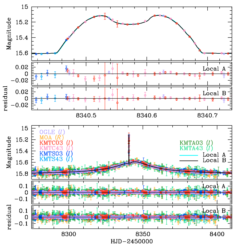
Figure 1 shows the light curve of OGLE-2018-BLG-1269. This light curve mostly follows a standard Paczyński (1986) curve except for the very short time interval , during which OGLE and KMTC observations caught a strong anomaly consisting of two strong spikes with a U-shaped trough. Such an anomaly typically occurs when a source crosses a pair of caustics formed by a binary lens with , i.e., a planetary system. Hence, we fit the light curve with the binary-lens single-source (2L1S) model.
In cases of standard 2L1S models, the lensing magnification, , can be described by seven nonlinear parameters. The first three are the geometric parameters : the time of closest lens-source approach, the impact parameter (scaled to the angular Einstein radius ), and the timescale, respectively. The next three are the parameters that describe the binarity of the lens: the projected companion-host separation (scaled to ), their mass ratio, and their orientation angle (relative to the source trajectory), respectively. The last parameter is the source radius , where is the angular source radius..
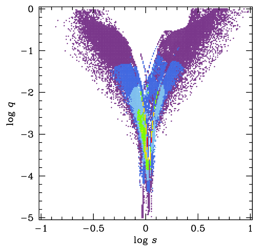
With these nonlinear parameters, we perform a systematic 2L1S analysis by adopting the modeling procedure of Jung et al. (2015). We first derive initial estimates of by fitting the single-lens single-source (1L1S) model to the event with the anomaly excluded. We also derive an initial estimate of based on the source brightness and from the 1L1S fit. Next, we carry out a dense search over a grid of , , and . For this, we divide the parameter space into grids in the range of , , and , respectively. At each grid point, we fix and then fit the light curve by allowing the remaining parameters to vary in a Markov Chain Monte Carlo (MCMC).
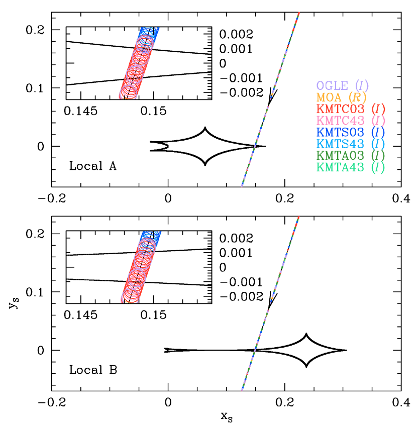
We identify two local minima in the resulting map in the plane (see Figure 2). We then further refine these minima by optimizing all fitting parameters, and finally find that they converge to the two points, i.e., and . See Table 1. The MCMC results shows that the best-fit parameters of the two solutions are consistent within (except for the separation ). However, the solution “Local A” () is disfavored relative to the solution “Local B” () by . In addition, the former solution has clear systematic residuals in the short-lived anomaly region as presented in the upper panel of Figure 1. Therefore, we exclude the “Local A” solution. The caustic structures for the two solutions are shown in Figure 3.
The timescale of the standard solution () comprises a substantial portion of Earth’s orbit period. Hence, we additionally check whether the standard fit further improves by introducing the microlens parallax (Gould, 1992, 2000),
| (1) |
where are the relative lens-source (geocentric proper motion, parallax). To account for the parallax, we add two parameters to the standard model, i.e., the north and east component of in equatorial coordinates. Note that the measurements of and allow one to determine the lens total mass and distance through the relations
| (2) |
where , is the source parallax, and is the source distance. Then, one can further determine the lens physical properties from the measured and , where is the physical projected companion-host separation.
The microlens parallax (due to the annual motion of Earth) can be partially mimicked by orbital motion of the binary lens (Batista et al., 2011). This implies that one should simultaneously consider the lens orbital motion when incorporating into the fit. Hence, we also model the orbital effect with two linearized parameters , which are the instantaneous change rates of and , respectively (Dominik, 1998).
Based on the “Local B” solution, we now fit the light curve with eleven fitting parameters . We also check a pair of solutions with and to consider the ecliptic degeneracy, which takes roughly (Skowron et al., 2011). From this modeling, we find that the two parameters are weakly constrained. We therefore only consider the MCMC trials that satisfy the condition . Here, is the projected kinetic to potential energy ratio (Dong et al., 2009)
| (3) |
where we adopt mas based on the distance to the giant clump in the event direction (Nataf et al., 2013).
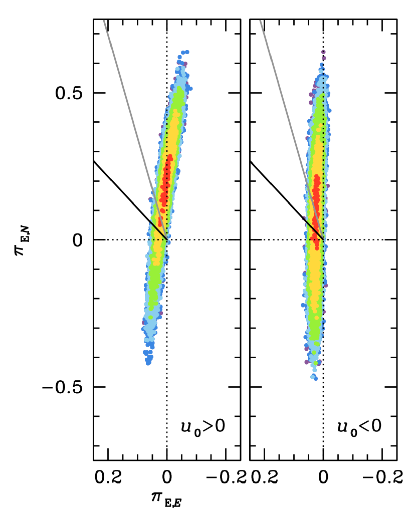
The results are listed in Table 1. We find that the addition of higher-order effects does not significantly improve the fit, which only provides . This implies that it is difficult to characterize the lens system from the fitted parallax parameters alone. Hence, we make a Bayesian analysis with Galactic model priors to constrain the lens physical parameters. Nevertheless, despite the low level of fit improvement, the analysis gives a strong one-dimensional (1-D) constraint on the parallax vector as seen in Figure 4. The short direction of these contours corresponds to the direction of Earth’s instantaneous acceleration at , namely (north through east), which induces an approximately antisymmetric distortion on the light curve around . In addition, the seven standard parameters are comparable between all the solutions (including the standard solution), with the exception of the sign of . Therefore, we take the measured microlens parallax into consideration in our Bayesian analysis (e.g., Jung et al. 2019).
4 Physical Parameter Estimates
4.1 Color-Magnitude Diagram (CMD)
The normalized source radius is precisely measured (see Table 1). This implies that we can measure provided that we can estimate the angular source radius . The Einstein radius is related to the lens mass and the relative parallax by
| (4) |
Then, we can use the measured to constrain the lens properties. Hence, we first estimate by following the approach of Yoo et al. (2004).
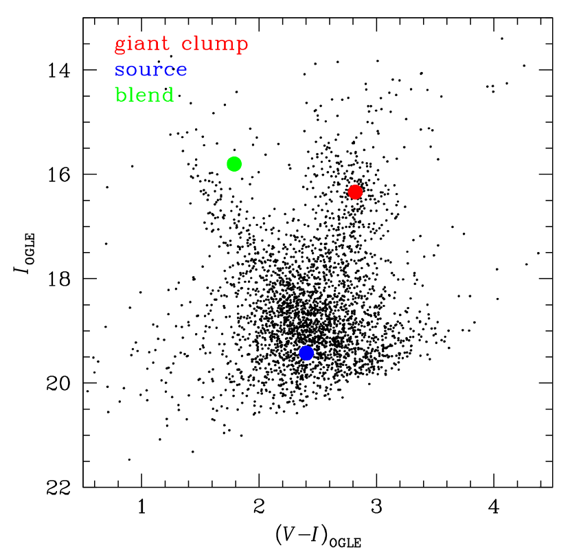
Based on the KMTC03 pyDIA reduction calibrated to the OGLE-III catalog (Szymański et al., 2011), we build a color-magnitude diagram (CMD) with stars centered on the event location (see Figure 5). We next find the source position of from the best-fit model. We also estimate the giant clump (GC) centroid as , which yields an offset
| (5) |
where is the intrinsic GC centroid (Bensby et al., 2013; Nataf et al., 2013). Using this offset, we obtain the dereddened source position as . This suggests that the source is either a late F or an early G dwarf.
We then apply to the relation (Bessell & Brett, 1988) and relation (Kervella et al., 2004) to derive
| (6) |
where we add error in quadrature to to account for the uncertainty of and the color/surface-brightness conversion of the Galactic-bulge population relative to locally calibrated stars. With the measured , we obtain
| (7) |
The geocentric relative lens-source proper motion is then
| (8) |
The unusually large values of and suggest that the lens lies in the Galactic disk. From the definition of (Equation (4)),
| (9) |
Thus, given the lens flux constraint, that will be discussed in the following subsection, the lens must be (unless the lens is black hole). We note that the measured is also consistent with the typical values of disk lenses.
4.2 Gaia PPPM of Baseline Object
Gaia data (Gaia Collaboration et al., 2016, 2018; Luri et al., 2018) will play a critical role in the derivation of the lens physical characteristics, in several different respects. As has become relatively common in recent years, we will make use of the Gaia proper-motion measurement of the “baseline object”. However, in contrast to most events with such a measurement, in this case, the baseline object is strongly dominated by the lens (or at least a stellar component of the lens system). Thus, the Gaia parallax measurement is also relevant111By contrast, Gaia parallax measurements of microlens sources, which are nearly all in the bulge, are of no practical use.. Moreover, we will in this paper, for the first time, make use of the Gaia position measurement of the baseline object. That is, we will use the full position, parallax, proper motion (PPPM) Gaia solution at various points in the analysis. Hence, we introduce all of these measurements here, together with some context and cautions on their use.
Gaia reports PPPM values (at epoch 2015.5) of (R.A.,Decl.)J2000 = (17:58:46.4171136073, :37:04.543560775) ,
| (10) |
and
| (11) |
Gaia also reports all correlation coefficients, but the only one of interest for our purposes is the one associated with the last equation, . Before continuing, we note that Gaia parallaxes have a color-dependent zero-point error. For relatively red stars (due to intrinsic color or reddening), the shift is measured to be (Zinn et al., 2019). Hence, we correct the baseline-object parallax to be
| (12) |
While the Gaia PPPM catalog is by far the best large-scale astrometric database ever constructed, its performance in the crowded fields of the Galactic bulge is not at the same level as in high-latitude fields, nor even as in the other parts of the Galactic plane. For example, Hirao et al. (2020) found that the Gaia proper-motion measurement of the baseline-object of OGLE-2017-BLG-0406 was spurious. This itself shows that Gaia measurements in crowded fields must be treated with caution.
However, Hirao et al. (2020) also showed, based on generally more precise (and likely, more accurate) OGLE proper motions of stars in the same field, that the reported Gaia proper motions of most stars are very reliable. In particular, after Hirao et al. (2020) eliminated stars with (which included OGLE-2017-BLG-0406S itself) and those with or , that only 1–2% of Gaia proper motions were outliers. However, the Gaia proper-motion errors had to be renormalized by a factor to enforce /dof = . Although the exact reason for this renormalization is not known, it is likely that bulge-field crowding is a major contributing cause. In particular, the Gaia mirror has an axis ratio of three, meaning that the Gaia point spread function (PSF) has the same ratio. Hence, as Gaia observes a field at various random orientations, light from faint ambient stars can enter the elongated PSF “aperture”, leading to “random” shifts in the astrometric centroid. This can lead to “excess noise” relative to the photon-based error estimates, and this “excess noise” is tabulated as the “astrometric excess noise sig (AENS)” parameter. In so far as this “excess noise” is truly “random”, it just degrades the measurement, which is reflected in the reported uncertainties. However, because it is likely due to real stars, whose positions change very little, and because the observing pattern is also not truly “random”, this “excess noise” can lead to systematic errors that are larger than the random errors.
In their study of Gaia proper-motion errors, Hirao et al. (2020) considered stars with AENS, so their results strictly apply to such stars. They did not notice any trends in behavior with AENS, and (though not specifically reported), they also did not notice any trends for AENS at a few times this level.
For OGLE-2018-BLG-1269, Gaia reports AENS=10.4. We therefore apply the Hirao et al. (2020) error renormalization to the above Gaia measurements. Although Hirao et al. (2020) only studied proper-motion errors (because this is the only quantity for which OGLE measurements are superior to Gaia), we apply this renormalization to all PPPM quantities.
For the position measurement, the formal errors are so small that they play no practical role, even after renormalization. So we ignore these errors. For the parallax measurement, the renormalized error is of the measured value. Hence, its role is mainly qualitative confirmation that the lens is nearby. The renormalized proper-motion errors () are still relatively small, and this measurement will play a crucial role at several points.
4.3 Blend is Due to Host and/or Its Companion
4.3.1 Gaia Baseline Object Is From Source
Gaia astrometry is generally given for epoch 2015.50, whereas the event peaked at 2018.61. In order to compare the position of the source (at 2018.61) with the position of the Gaia baseline object at the same time, we first propagate the positions of all Gaia stars (including the baseline object) forward in time by yr. That is, for each star in the field, , we calculate,
| (13) |
where is the proper motion of Gaia object. We then cross-match the Gaia and KMTNet pyDIA catalogs within a square, excluding entries that fail a relatively forgiving cut on an empirical color-color relation, and with a astrometric cut (to allow for optical distortion of the KMTNet camera). Next, we fit for a transformation from Gaia to KMTNet pyDIA coordinates using all matches obtained from the previous step, except the “baseline object”, by minimizing the unrenormalized ,
| (14) |
where is a -th order polynomial transformation, i.e., , , and parameters for .
We find that the results vary very little but the polynomial fit is slightly better than the others. We recursively eliminate outliers, of which there are objects222We note that roughly half are false matches due to the relatively loose matching criteria, and the remainder are likely due to corrupted astrometry from unresolved objects. for 487 original matches. The scatter is mas, which is almost an order of magnitude larger than the typical formal propagated errors in . Although the errors are probably somewhat underestimated in crowded fields (Hirao et al., 2020), it is still the case that this scatter is completely dominated by the errors of KMTNet pyDIA astrometry.
We then apply the resulting transformation to the propagated blend position , and subtract this from the pyDIA source position that is derived from difference images:
| (15) |
The error comes from three sources added in quadrature: error in the transformation coefficients (mas), error in the propagated value of (mas), and error in the pyDIA measurement of (mas).
That is, the Gaia baseline object lies mas from the source at the time of the event. We repeat this exercise using OGLE data and obtain mas, which confirms that the source and the Gaia baseline object are very close.
4.3.2 Probability of Chance Superposition is
Figure 5 shows that the blend is bright and belongs to the foreground main-sequence branch, i.e., . The surface density of such “bright” , “blue” foreground stars is only . In the previous subsection, we showed that the Gaia baseline object is within mas. Therefore, the probability of an unrelated bright foreground star lying within of this foreground-star lens is . Hence, the blend is almost certainly associated with the event, rather than being a random interloper.
4.3.3 Blended Light is Due to the Lens System
That is, there are broadly five classes of objects that could contribute significantly to baseline object: (0) the source, (1) a stellar companion to the source, (2) the lens host, (3) a stellar companion to the host, (4) an unrelated ambient star.
Of course, the source does contribute, but this contribution is well determined from the microlensing fit, and in the present case is also quite small. The remaining four possibilities are candidates for the remaining light, i.e., the blend. The probability just calculated implies that (4) is ruled out. Moreover (1) is also ruled out by the color ( mag bluer than the clump) and magnitude ( mag brighter than the clump). To be a companion of the source (and hence in the bulge) this would have to be a late B dwarf, of which there are essentially none in the bulge (apart from the star-forming regions near the Galactic Center).
Thus, the blended light is due to either the host, a companion to the host, or possibly a combination of the two. For any of these possibilities, the parallax and proper motion of the host are essentially equal the parallax and proper motion of the blend because the host and it putative companion are at essentially the same distance, and their orbital motion is very slow compared the lens-source relative motion. Hence, the Gaia measurements of these quantities will act as strong constraints on the estimates of the physical parameters of the lens system.
4.4 Bayesian Analysis
For the Bayesian analysis, we will incorporate the Gaia astrometric measurements in addition to the usual microlensing-parameter measurements.
4.4.1 Inputs From Gaia
To do so, we first note that for the three parameters measured by Gaia, the observed (“baseline object”) quantities are related to the underlying physical (“source” and “lens”) quantities333In the more general case, one would write “source” and “blend”. However, in Section 4.3.3, we established that the blend is the lens (although up to this point it is not yet clear whether it can be identified with the host, its stellar companion, or both). by (Ryu et al., 2019)
| (16) |
where is the flux fraction of the source in the Gaia band and are the flux of the source and the baseline object, respectively. We estimate by noting that the peak of the Gaia passband is broadly consistent with that of the band and the typical photometric error of Gaia observation is . We thereby estimate based on our result that the blend is mag brighter than the source in the band.
To find the lens parallax , we adopt from Nataf et al. (2013) and we renormalize the errors (by a factor ) in Equation (12) to obtain . We then apply Equation (16) to and find
| (17) |
The situation is substantially more complicated for the proper motion. First, the microlensing solution gives the amplitude of the lens-source relative proper motion in the geocentric frame, but the Gaia proper motion is in the heliocentric frame. We can relate these by
| (18) |
where is the projected velocity of Earth at and are the heliocentric proper motions of the lens and the source, respectively.
In principle, we could fully incorporate Equations (16) and (18) into the Bayesian analysis below. However, as we now show, for the case of OGLE-2018-BLG-1269 the lens proper motion is well approximated by .
First, we combine Equations (16) and (18) to yield
| (19) |
Next, we note that for typical final values of , we have , and hence, regardless of the direction of , we have . Therefore, the second term in the first entry of Equation (19) is of order , which is a factor of about four smaller than the renormalized errors in (). Hence, we adopt . Then, after renormalizing the errors (by a factor ) in Equation (11) and rotating to Galactic coordinates, we obtain
| (20) |
4.4.2 Bayesian Formalism
With the four measured constraints , we now make a Bayesian analysis following the procedure of Jung et al. (2018). We first build a Galactic model with models of the mass function (MF), density profile (DP), and velocity distribution (VD) of astronomical objects. For the MF and DP, we adopt the models used in Jung et al. (2018). For the VD, we use the proper motion distribution of stars measured by . For the source proper motion, we examine a CMD using red giant stars within centered on the event direction and find their mean proper motion and standard deviation in Galactic coordinates
| (21) |
For the lens proper motion, we employ Equation (20).
For each solution of and , we draw one billion random events based on the adopted Galactic model. For each random event , we then infer the four parameters and find the difference between the inferred and the measured values, i.e.,
| (22) |
where is the inferred parallax, and and are the measured and its covariance matrix, respectively. We next find the likelihood of the event by , where is the lensing event rate.
For each random event , we also infer the lens position in the calibrated CMD, i.e., , in order to check whether the lens flux predicted from the Bayesian estimates is consistent with the blended flux. For this, we first construct a set of isochrones with different metallicities and ages (Spada et al., 2017), i.e., with and Gyr. In each isochrone , we next estimate the absolute -band magnitude and intrinsic color of the lens from the inferred lens mass . We then find the dereddened lens magnitude in the and band by = and = . We next estimate the extinction to the lens using the partial extinction model (Bennett et al., 2015; Beaulieu et al., 2016),
| (23) |
where the index denotes the passband and is the dust scale height. Here is the extinction to the source, for which we adopt and from our CMD analysis (Equation (5)). We then derive using , and bin the CMD by these lens positions with the likelihood .
We emphasize that in this initial analysis, we completely ignore constraints coming from the blended light. That is, we neither impose any constraint on the lens light (such as not to exceed the blended light) nor consider the possibility that the lens is responsible for the blended light. At this point, we simply “predict” the lens color and magnitude based on the [or ] constraints together with the Galactic model and model isochrones. We investigate the role of the blended light in constraining the solution only after comparing these predictions to the observed blended light.
4.4.3 Bayesian Results
We finally investigate the posterior probabilities of the lens properties from all random events. We note that to check the contribution of the constraint on the Bayesian estimates, we also explore the posterior probabilities with constraints.
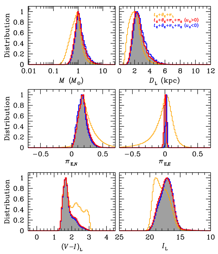
The results from the constraints are shown in Figure 6 and listed in Table 2. Also listed are the total Galactic-model probability and the net relative probability , where is the relative fit probability and is the difference between the two solutions. Here, is the orientation angle of .
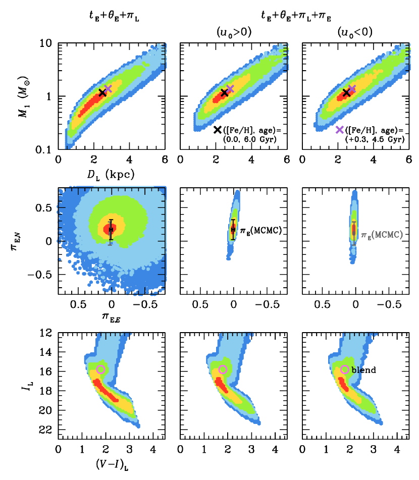
We find that the measured from modeling gives a strong constraint on the probability distributions. However, we also find that the host-mass ranges of the two solutions ( and ) are somewhat different from each other. Because is the only prior constraint that differs significantly between the two solutions and because is connected to the lens mass (Equation (2)), the difference would imply that the Galactic-model priors disfavor one of the solutions. To check this, we also draw the two-dimensional (-D) likelihood for the lens parameters obtained from the and the constraints. See Figure 7. We note that the black and grey error bars in the three planes are the errors of listed in Table 1 for the and solutions, respectively. From this figure, we find that the measured from both and solutions are consistent at the level. This mutual consistency is reflected in the almost equal values of (ratio ) in Table 2. Thus, our estimates should reflect the weighted average of the two solutions, although these hardly differ.
Hence, these results, which do not yet incorporate constraints from the blended light, suggests that the host is a Sun-like star with located at a distance of . Then, the microlensing companion is a planet with separated (in projection) from the host by . That is, the planet is a cold giant lying beyond the snow line, i.e., .
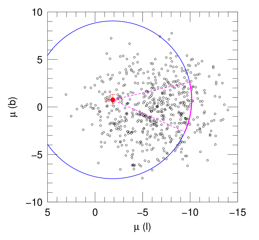
It is of some interest to understand how the Bayesian analysis constrains the lens mass to a range of a factor at the level despite the fact that varies by a factor at (see Figure 4), while . The main reason is that the direction of (and so the direction of ) is reasonably well constrained by the Gaia measurement of together with the relatively large value of . This is illustrated in Figure 8, which shows and a blue circle to represent all possible that are consistent with . The magenta arc of this circle represents the range of as given by Equation (21). The arc of allowed (at ) directions is shown by dashed lines. This same arc, rotated to Equatorial coordinates (and displayed as lens-source rather than source-lens motion) is shown in Figure 4, with boundaries to (north through east). The first point to note is that, for both and , this arc subtends a region that is almost entirely contained within the contours, implying mutual consistency between two constraints on the direction that are entirely independent. Second, for the contours, which are almost perfectly vertical, we can evaluate the range of as . This confirms that the relatively tight constraints on in the Bayesian analysis derive from the application of the directional constraint on lens-source relative motion (Figure 8) to the -D parallax contours from the light-curve analysis (Figure 4). That is, the Bayesian mass estimate comes primarily from a combination of measured microlensing parameters and measured lens proper motion, while the Galactic model enters mainly by constraints on the source proper motion.
5 Blended Light Is Due Mainly to the Host
As we discussed in Section 4, the facts that the lens host is known (from the Bayesian analysis) to be a roughly solar-mass foreground-disk star and that there is such a roughly solar-mass foreground-disk star projected within mas of the lens make it virtually certain that this blended light comes from the lens system. That is, the blended light must be due to the host, to a companion to the host, or to some combination of the two. Here we examine this issue in detail.
The two lower-right panels of Figure 7 show that the blend (magenta circle) lies at about from the most likely “prediction” of the Bayesian analysis for both the and solutions. However, this nominal “discrepancy” may simply reflect the fact that stars spend far more time on the upper main sequence than they do at the location of the blend (i.e., subgiant branch, or possibly end of the turnoff). That is, a small range of lens masses from the upper main-sequence is projected onto a small region of the CMD, but an equally small range of masses that are just slightly larger are projected all across the subgiant branch, and thus populate the CMD at much lower density. Hence, the blended light could be fully consistent with being due to the host, but would show up as “relatively low probability” on this figure.
We now must take account of the fact that, despite the low prior probability that the host is a turnoff/subgiant star (as indicated by it being projected against the green contours in Figure 7), there is actually such a “star” associated with the event, i.e., either the host itself, a companion to the host, or a combination of the two. We now consider these three possibilities in turn.
5.1 Blend is Consistent with Being Due to the Host
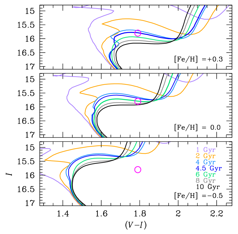
We first ask whether the host is consistent with being the primary contributor to the blended light? If it is, then there must be a star simultaneously consistent with the microlensing properties and the blended light. For this analysis, we use the measured Einstein radius and the adopted source parallax (Equation (2)) to map a set of model isochrones to the calibrated CMD. Given and , we can take a star with given mass , intrinsic color , and absolute magnitude , to estimate the distance to the star . We next find the dereddened - and -band magnitudes by = and = . We then find the position of the star in the calibrated CMD using the partial extinction model (Equation (23)). Finally, we build an “observed” isochrone with from all stars listed in the model isochrone. For the three cases of , we then construct “observed” isochrones with different ages, and compare them to the blended light to estimate the blend mass and distance .
We find that two “observed” isochrones can match the blended light (see Figure 9). That is, the two curves for and pass through the blend position with the offset of , respectively. The estimated mass and distance to the blend are for and for . These estimates imply that for typical disk populations with , and are in the range of and , respectively. These ranges show remarkable agreement with the prediction from the Bayesian analysis (see Figure 7). This implies that the host is consistent with causing the blended light, which is then a subgiant (or possibly late turnoff) star.
5.2 Blend as Stellar Companion to the Host (Qualitative Analysis)
We still must consider the possibility that the blended light is primarily due to a stellar companion to the host, rather than the host itself. That is, it is due to a star that does not directly enter into the microlensing event but is gravitationally bound to the host. This alternative explanation for the blended light can be conceptually divided into two cases: either the host contributes very little light to the blend, or the host and its brighter stellar companion both contribute significantly to the observed blended light. When we quantitatively evaluate the probability that the host dominates the blended light, we will treat these two alternative cases as a single case. However, in the qualitative treatment that follows immediately below, we make a conceptual distinction between them.
In order to evaluate the three possibilities, i.e., that the blend light
-
(1)
is dominated by host
-
(2)
is dominated by a stellar companion to the host (and the host contributes relatively little light),
-
(3)
receives comparable contributions from the host and a stellar companion.
we first divide all single and binary systems containing a subgiant (or possibly late turnoff) star into six classes:
-
(A)
single stars,
-
(B)
binaries with orbital periods day
-
(C)
binaries with orbital periods day
-
(D)
binaries with , and mass ratios ,
-
(E)
binaries with , and ,
-
(F)
binaries with , and .
Using the statistics of Duquennoy & Mayor (1991) for solar-type stars, we estimate relative fractions for the classes , respectively.
These six classes of systems can contribute the three cases of events as follows. Class (A) can contribute only to events of case (1). Class (B) cannot contribute to any events with a OGLE-208-BLG-1269 type light curve because companions in this period range would have given rise to recognizable signals in the light curve (days) or would violate the -based source-blend separation measurement (days).
Class (C) is excluded for cases (2) and (3) because the centroid of light would be displaced from the the host (and therefore the host) by more than mas. However, it is permitted for case (1) because the light from the companion would not significantly displace the light centroid.
Class (D) can contribute to events of case (1) but not of case (2) or (3). That is, the light contributed by the stellar companion would not be enough to qualitatively alter the photometric appearance of the combined light relative to an isolated turnoff/subgiant star, so case (1) is compatible. However, the mass of the host for case (2) is too low to be compatible with microlensing constraints (see Table 2). Therefore, case (2) is excluded. And case (3) is also excluded because a companion cannot contribute significantly.
Class (E) can contribute to either case (1) or case (2). Because the two stars in the lens system must be on the same isochrone, in the class (E) mass-ratio range, the more massive star must be above the turnoff and the less massive one must be below the turnoff. Hence, they differ by at least one magnitude, which implies that they contribute substantially differently to the total light of the blend. From the lower-right panels of Figure 7, it is clear that over most of this mass-ratio range, the lower-mass star would have a similar color to the blend. Hence, the brightness of the higher-mass star would be reduced by to mag, while its color would hardly be altered, relative to the blend. Thus, its position on the CMD would be essentially the same as that of the blend. In particular, it would be projected against the same green contours, and, in fact, slightly closer to the yellow contours.
Because class (F) systems can contribute only to case (3), we can now qualitatively evaluate the relative likelihood of case (1) (blended light from “turnoff/subgiant star” is dominated by the host, i.e., classes (A), (C), (D), and part of class (E)) and case (2) (blended light from “turnoff/subgiant star” is dominated by a companion to the host, i.e., part of class (E)). Then we will return to case (3).
For class (E), in which there are two stars in the system, i.e., higher- and lower-mass stars, the overall probability of lensing is higher than for a single star by because there are two well-separated lenses that could give rise to the event. And the relative probability of the lower-mass star giving rise to the event is . Therefore, relative to single-host case, the absolute lensing probabilities of two stars scale as and , respectively. We can then approximate the lower-mass events of class (E) by . Then, the probability for case (2) relative to case (1) can be directly evaluated: .
Naively, event case (3) appears highly disfavored because only system class (F) contributes to it, and this comprises only of all systems. In fact, however, this case requires close examination for proper evaluation.
We first consider the very special subcase that the host and its companion are identical. Then their colors would be the same as the blend, but their magnitudes would be mag fainter than the blend. In principle, this might have put them on the main sequence. In this case, the low relative probability of such binary systems () would have been counterbalanced by the fact that main-sequence stars are far more common than turnoff/subgiants of the same color. In fact, however, Figure 9 shows that this position ( mag below the blend) is not inhabited by stars on any or the fairly broad range of isochrones that we have displayed.
If we consider the broader case of approximately (rather than exactly) equal masses for the two components (), we see that essentially the same (above) argument applies to the case. The less massive star will be fainter and bluer than the blend, while the more massive star will be fainter and redder. The upper panel of Figure 9 shows that at , it is possible for a star to exist on, e.g., the -Gyr isochrone that is mag fainter and somewhat redder than the blend. However, this position invalidates the main advantage of event cases that was just mentioned above: the lens (or its companion) remains a subgiant and is not on the more populous main sequence. Hence, the probability of this solution is very low. Using the same procedure as above, we derive .
5.3 Blend as Lens Companion (Quantitative Analysis)
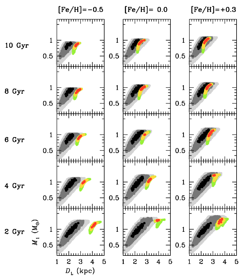
We now conduct a quantitative analysis aimed at both testing the qualitative ideas presented above and deriving a more precise quantitative result. Our starting point is to draw random events from the same Galactic model used for the Bayesian analysis described above and to weight each event by the same priors. However, for each simulated event, we either “accept” or “reject” it according to whether the combined light from the host and some companion drawn from the same isochrone is compatible with the blended light. That is, each simulated event has a corresponding -band magnitude and color; if there exists a companion along the same isochrone for which the combined light is compatible with the blend, the event is “accepted”. The entire isochrone is reddened in the same manner as was done for the case that the blend is dominated by the host light. We consider the same isochrones that were analyzed for the host=blend case, i.e., case (1). We note that after investigating these separate-isochrone cases, we must still combine them to obtain an overall relative probability of case (1) versus cases (2)+(3). This step will also require incorporating information about binary frequency.
Figure 10 shows separate contours, in the lens mass-distance plane, for the all [accepted+rejected] (black, dark grey, grey) and [accepted-only] (red, yellow, green) simulated events. We first focus on the five isochrones. These show that the accepted contours lie well away from the contours for all trials in each of the panels. This implies that a very small fraction are accepted. Numerically, we find that the -, -, and -Gyr isochrones have the highest rate of acceptance: about for each (see Table 3). To the extent that these do not overlap (which is partial), they would add constructively. Thus, these three isochrones contribute about . The other two isochrones contribute negligibly.
We next focus on the isochrones. Again, the oldest three isochrones contribute the most. However, such old, very metal rich stars are very rare within a few kpc of the Sun. Hence, we ignore these. The two youngest isochrones together contribute .
Lastly, we examine the solar-metallicity isochrones. These contribute for the Gyr isochrones, respectively. However, -Gyr solar-metallicity stars are extremely rare, and -Gyr solar-metallicity stars are fairly rare, so we make an overall estimate of for solar metallicity stars. We note that the two youngest isochrones contribute negligibly.
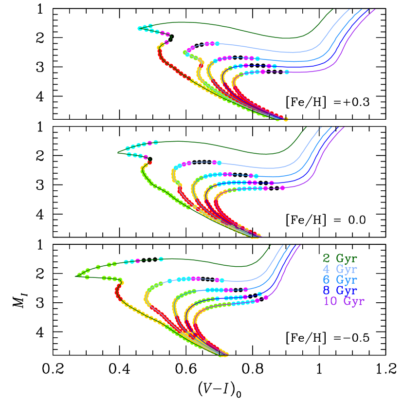
Next, we examine Figure 11, which shows where hosts (red, yellow, green) and stellar companions (black, magenta, cyan) lie on the theoretical isochrones for all isochrone cases. We note that only “accepted” events are shown. The most important feature of these diagrams is that the stellar companion tracks are almost all confined to the subgiant branch. This confirms the basic logic of the approach that we outlined in the enumeration in Section 5.2, i.e., of considering the relative probability of systems that contain a subgiant-branch star. Recall that if the stellar companion were on the main-sequence for case (3), but it were on the subgiant branch for case (2), then we would need to take account of the fact that main-sequence stars are more common than subgiants.
Now, the companion is actually on the main sequence for the top two -Gyr isochrones, and it is on the turnoff for the metal rich -Gyr isochrone. However, recall from Figure 10 that the former contributes negligibly and the latter contributes . Even if this percentage were augmented by a factor due to slower evolution on the turnoff, its contribution would still be small.
Thus, considering that both and can contribute to case (1) as discussed in Section 5.1, while of stellar populations at these metallicities can contribute to cases (2)+(3), we estimate that from this quantitative analysis alone, the probability for cases (2)+(3) relative to case (1) is .
We now must take account of the fact that Classes (A), (C), (D), and (E) can contribute to case (1), while Classes (E) and (F) can contribute to cases (2)+(3). This contributes a relative probability of , i.e., . Therefore, the “total probability” that the host dominates the blend light is .
Finally, we ask why the quantitative analysis gave much more certainty (“”) that the host dominates the blended light than the qualitative analysis? The primary reason is that in the qualitative analysis, we implicitly assumed that, for most cases, there would be some isochrone that could provide the “extra light” from a turnoff/subgiant star that could be added to the host to make the observed blended light. However, Figure 10 shows that this is not the case.
6 Discussion
We have shown that the bright, relatively blue blended light is very likely to be primarily due to the host. The blend, and thus almost certainly the host, can be basically characterized immediately from a medium-resolution spectrum taken on a , or even class telescope. This would also provide a first epoch for the radial-velocity signatures of a putative stellar companion to the blend. Moreover, by taking a high-resolution spectrum on an class telescope (similar to those obtained by Bensby et al. 2013), one could make a very detailed study of the chemical composition, age and mass of the blend/host.
Finally, future radial-velocity observations with class telescopes could potentially detect and further characterize the planet. For example, let us assume that host and planet have , as in the example of the 6-Gyr, isochrone analyzed in Section 5.1. Then, we may estimate a semi-major axis, , i.e., very similar to our own Jupiter. In this case, the period would be yr, and reflex velocity of the host would be . While the amplitude of this variation will be further reduced by , it should still be measurable on class telescopes. Because we already know , these measurements would enable determination of the inclination angle , in addition to the period and the eccentricity , which are rarely if ever possible for microlensing planets.
OGLE-2018-BLG-1269Lb is the second microlensing planet with a bright blue host for which such spectroscopic studies on telescopes will be possible. The first was OGLE-2018-BLG-0740b (Han et al., 2019), which also had a bright, blue blend due to a host. In that case, the host was more than one magnitude fainter in the band, but just mag fainter in the band compared to OGLE-2018-BLG-1269Lb. On the other hand, the planet-host mass ratio was substantially larger, leading to an estimated reflex velocity that was times larger. Taking all these factors into account, OGLE-2018-BLG-0740Lb and OGLE-2018-BLG-1269Lb are comparably feasible for future radial-velocity studies444The first microlensing planets for which m telescope radial-velocity studies were proposed were OGLE-2006-BLG-109Lb,c. At , their host is much less massive, hence much redder and fainter than either of the bright blue hosts discussed here. Nevertheless, Bennett et al. (2010) estimated that the host had and so proposed that it would be possible to monitor it in the infrared with m telescopes..
References
- Alard & Lupton (1998) Alard, C., & Lupton, Robert H. 1998, ApJ, 503, 325
- Albrow et al. (2009) Albrow, M. D., Horne, K., Bramich, D. M., et al. 2009, MNRAS, 397, 2099
- Alcock et al. (2001) Alcock, C., Allsman, R. A., Alves, D. R., et al. 2001, Nature, 414, 617
- Batista et al. (2015) Batista, V., Beaulieu, J.-P., Bennett, D. P., et al. 2015, ApJ, 808, 170
- Batista et al. (2011) Batista, V., Gould, A., Dieters, S., et al. 2011, A&A, 529, 102
- Beaulieu et al. (2016) Beaulieu, J.-P., Bennett, D. P., Batista, V., et al. 2016, ApJ, 824, 83
- Bennett et al. (2015) Bennett, D. P., Bhattacharya, A., Anderson, J., et al. 2015, ApJ, 808, 169
- Bennett et al. (2020) Bennett, D. P., Bhattacharya, A., Beaulieu, J. P.,et al. 2020, AJ, 159, 68
- Bennett et al. (2010) Bennett, D. P., Rhie, S. H., Nikolaev, S., et al. 2010, ApJ, 713, 837
- Bensby et al. (2013) Bensby, T., Yee, J. C., Feltzing, S., et al. 2013, A&A, 549, 147
- Bessell & Brett (1988) Bessell, M. S., & Brett, J. M. 1988, PASP, 100, 1134
- Bhattacharya et al. (2018) Bhattacharya, A., Beaulieu, J.-P., Bennett, D.P., et al. 2018, AJ, 156, 289
- Bond et al. (2001) Bond, I. A., Abe, F., Dodd, R. J., et al. 2001,MNRAS, 327, 868
- Dominik (1998) Dominik, M. 1998, A&A, 329, 361
- Dong et al. (2009) Dong, S., Gould, A., Udalski, A., et al. 2009, ApJ, 695, 970
- Duquennoy & Mayor (1991) Duquennoy, A., & Mayor, M. 1991, A&A, 248, 485
- Gaia Collaboration et al. (2018) Gaia Collaboration, Brown, A. G. A., Vallenari, A., et al. 2018, A&A, 616, 1
- Gaia Collaboration et al. (2016) Gaia Collaboration, Prusti, T., de Bruijne, J. H. J., et al. 2016, A&A, 595, A1
- Gaudi et al. (2008) Gaudi, B. S., Bennett, D. P., Udalski, A., et al. 2008, Sci, 319, 927
- Gould (1992) Gould, A. 1992, ApJ, 392, 442
- Gould (2000) Gould, A. 2000, ApJ, 542, 785
- Griest et al. (1991) Griest, K. et al. 1991, ApJ, 372, L79
- Han et al. (2018) Han, C., Jung, Y. K., Udalski, A., et al. 2018, ApJ, 867, 136
- Han et al. (2019) Han, C., Yee, J. C., Udalski, A., et al. 2019, AJ, 158, 102
- Hirao et al. (2020) Hirao, Y., Bennett, D.P., Ryu, Y.-H., et al., 2020, in press, arXiv:2004.09067
- Jung et al. (2019) Jung, Y. K., Gould, A., Zang, W., et al. 2019, AJ, 157, 72
- Jung et al. (2018) Jung, Y. K., Udalski, A., Gould, A., et al. 2018, AJ, 155, 219
- Jung et al. (2015) Jung, Y. K., Udalski, A., Sumi, T., et al. 2015, ApJ, 798, 123
- Kervella et al. (2004) Kervella, P., Bersier, D., Mourard, D., et al. 2004, A&A, 428, 587
- Kim et al. (2018) Kim, D.-J., Kim, H.-W., Hwang, K.-H., et al. 2018, AJ, 155, 76
- Kim et al. (2016) Kim, S.-L., Lee, C.-U., Park, B.-G., et al. 2016, JKAS, 49, 37
- Kozłowski et al. (2007) Kozłowski, S., Woźniak, P. R., Mao, S., & Wood, A. 2007, ApJ, 671, 420
- Luri et al. (2018) Luri, X., Brown, A. G. A., Sarro, L. M., et al. 2018, A&A, 616, A9
- Nataf et al. (2013) Nataf, D. M., Gould, A., Fouqué, P., et al. 2013, ApJ, 769, 88
- Paczyński (1986) Paczyński, B. 1986, ApJ, 304, 1
- Paczyński (1991) Paczyński, B. 1991, ApJ, 371, L63
- Ryu et al. (2019) Ryu, Y.-H., Navarro, M.G., Gould, A. et al. 2019, AJ, 159, 58
- Skowron et al. (2011) Skowron, J., Udalski, A., Gould, A., et al. 2011, ApJ, 738, 87
- Spada et al. (2017) Spada, F., Demarque, P., Kim, Y.-C., et al. 2017, ApJ, 838, 161
- Sumi et al. (2003) Sumi, T., Abe, F., Bond, I. A., et al. 2003, ApJ, 591, 20
- Szymański et al. (2011) Szymański, M. K., Udalski, A., Soszyński, I., et al. 2011, AcA, 61, 83
- Tomaney & Crotts (1996) Tomaney, A.B. & Crotts, A.P.S. 1996, AJ, 112, 2872
- Udalski (2003) Udalski, A. 2003, Acta Astron., 53, 291
- Udalski et al. (2015) Udalski, A., Szymański, M. K., & Szymański, G. 2015, AcA, 65, 1
- Vandorou et al. (2019) Vandorou, A., Bennett, D. P., Beaulieu, J.-P., et al. 2019, arXiv:1909.04444
- Woźniak (2000) Woźniak, P. R. 2000, AcA, 50, 42
- Yee et al. (2016) Yee, J. C., Johnson, J. A., Skowron, J., et al. 2016, ApJ, 821, 121
- Yoo et al. (2004) Yoo, J., DePoy, D. L., Gal-Yam, A., et al. 2004, ApJ, 603, 139
- Zinn et al. (2019) Zinn, J. C., Pinsonneault, M. H., Huber, D., & Stello, D. 2019, ApJ, 878, 136
| Parameters | Local A | Local B | ||
|---|---|---|---|---|
| Standard | Standard | Orbit+Parallax | ||
| /dof | 22266.3/21841 | 22229.4/21841 | 22221.2/21837 | 22222.1/21837 |
| () | 8343.876 0.025 | 8343.849 0.025 | 8343.903 0.030 | 8343.895 0.029 |
| 0.141 0.026 | 0.142 0.023 | 0.144 0.028 | -0.143 0.024 | |
| (days) | 70.792 1.064 | 70.584 0.923 | 70.672 1.661 | 69.597 1.172 |
| 1.032 0.019 | 1.126 0.012 | 1.123 0.032 | 1.124 0.033 | |
| () | 5.940 0.063 | 5.932 0.066 | 5.753 0.264 | 5.957 0.230 |
| (rad) | 1.888 0.026 | 1.887 0.026 | 1.887 0.069 | -1.891 0.068 |
| () | 5.886 0.097 | 5.917 0.092 | 5.895 0.177 | 5.941 0.130 |
| – | – | 0.171 0.150 | 0.114 0.173 | |
| () | – | – | 0.086 0.217 | 0.253 0.107 |
| (yr-1) | – | – | -0.287 0.319 | -0.219 0.298 |
| (yr-1) | – | – | 0.032 0.554 | 0.205 0.492 |
| 0.270 0.006 | 0.270 0.005 | 0.275 0.007 | 0.273 0.006 | |
| 7.303 0.006 | 7.304 0.005 | 7.299 0.007 | 7.301 0.006 | |
| Parameters | Weighted | ||
|---|---|---|---|
| (au) | |||
| (kpc) | |||
| (deg) | |||
| 1.0 | 0.64 | – | |
| 416913.4 | 382315.5 | – | |
| 416913.4 | 244681.9 | – |
| age (Gyr) | |||
|---|---|---|---|