Old Wine in a New Bottle:
Technidilaton as the 125 GeV Higgs
– Dedicated to the late Professor Yoichiro Nambu¹¹1deceased on July 5, 2015—

This talk is an impromptu substitute filling the hole of the cancellation of the talk to be given by Volodya Miransky, my old friend, so this is a kind of personal sentiments style rather than a scientific presentation. Sorry for that in advance.

History repeats itself: At the first SCGT workshop in 1988 motivated by our work [1, 2] proposing the walking technicolor based on his paper [3], the Volodya’s talk was also cancelled, although he was a frequent repeater to many (out of ten) SCGT workshops during the long period more than a quarter century 1988 - 2015.

Volodya discovered [3] so-called Miransky scaling:

$$m_{F}\simeq 4\Lambda\cdot\exp\left(-\frac{\pi}{\sqrt{\frac{\alpha}{\alpha_{\rm cr}}-1}}\right)\,\ll\Lambda\quad\left(\frac{\alpha}{\alpha_{\rm cr}}-1\ll 1\right)$$

(1)

in the scale-invariant gauge model (ladder model), an essential singularity scaling analogous to the Berezinsky-Kosterlitz-Thouless phase transition (what we called “conformal phase transition” [4]), where $m_{F}(\neq 0)$ is the spontaneous chiral symmetry breaking (S$\chi$SB) solution of the ladder Schwinger-Dyson (SD) gap equation for the fermion and $\Lambda$ is the ultraviolet cutoff to regularize the theory to act as an intrinsic scale $\Lambda_{\rm TC}$ of the walking technicolor, similarly to the $\Lambda_{\rm QCD}$ in QCD, responsible for the trace anomaly $\theta_{\mu}^{\mu}\propto\Lambda^{4}$ as the explicit breaking of the scale symmetry manifesting itself as the running of the coupling in the ultraviolet region far bigger than the S$\chi$SB scale $m_{F}$.

The S$\chi$SB solution exists only in the strong coupling phase $\alpha>\alpha_{\rm cr}\neq 0$, where the non-zero critical coupling $\alpha_{\rm cr}\neq 0$ discovered by Maskawa-Nakajima [5] is the characterization of the strong coupling gauge theories (SCGT). It is a gauge analogue of the non-zero critical coupling, $G^{(\rm NJL)}>G_{\rm cr}\neq 0$, of the Nambu-Jona-Lasinio (NJL) model [6], which, despite the resemblance, should actually be distinguished from the BCS dynamics having zero critical coupling $G_{\rm cr}^{(\rm BCS)}=0$ (weak coupling theory in broken phase even for infinitesimal coupling).³³3 The characteristic weak coupling of the BCS theory is due to the existence of the Fermi surface where the fermions are effectively in the 2-dimensional brane instead of 4 dimensional free space bulk, whereas the Cooper pairs and Nambu-Goldstone (NG) modes are bosons and hence live in the bulk to trigger the Higgs mechanism (Meissner effect), escaping the Mermin-Wagner-Coleman theorem in genuine 2 dimensional theories.

Volodya further invented nonperturbative renormalization [3] taking $\Lambda\rightarrow\infty$ as $m_{F}={\rm fixed}$ for the Miransky scaling Eq.(1), which yields a nonperturbative beta function: [8]

	$\displaystyle\beta^{(NP)}(\alpha)$	$\displaystyle=$	$\displaystyle\Lambda\frac{\partial\alpha(\Lambda)}{\partial\Lambda}\Bigg{|}_{m_{F}}=-\frac{2\pi^{2}\alpha_{\rm cr}}{\ln^{3}(\frac{4\Lambda}{m_{F}})}=-\frac{2\alpha_{\rm cr}}{\pi}\left(\frac{\alpha}{\alpha_{\rm cr}}-1\right)^{\frac{3}{2}},$		(2)
	$\displaystyle\alpha(\mu)$	$\displaystyle=$	$\displaystyle\alpha_{\rm cr}\left[1+\frac{\pi^{2}}{\ln^{2}(\frac{\mu}{m_{F}})}\right]\,,\quad(\alpha>\alpha_{\rm cr}\neq 0)$		(3)

Thus the coupling actually starts running nonperturbatively once the $m_{F}\neq 0$ is generated, even if the initial ladder coupling is scale-invariant (nonrunning). Besides the explicit breaking by the intrinsic scale $\Lambda$, the scale symmetry is now explicitly broken also by $m_{F}$ which was generated by the spontaneous breaking of the scale symmetry, with the new trace anomaly (nonperturbative trace anomaly) $|{\theta_{\mu}^{\mu}}^{(NP)}|={\cal O}(m_{F}^{4})(\ll\Lambda^{4})$. From Eq.(2) we can see that the $\alpha_{\rm cr}\neq 0$ is regarded as a nontrivial ultraviolet fixed point, although the input ladder coupling $\alpha(\mu^{2})=\alpha$ in the infrared region $\mu^{2}<\Lambda^{2}=\Lambda_{\rm TC}^{2}$ is regarded as the nontrivial infrared fixed point. This opened a new phase of the SCGT for the composite model and turned out to be the basics of the whole walking dynamics.

We applied this Volodya’s result to the technicolor theory, and proposed what we called “Scale-invariant Technicolor” (now called Walking Technicolor) [1, 2], where we found a large anomalous dimension

$$\gamma_{m}=1\,\quad\quad(\alpha>\alpha_{\rm cr})$$

(4)

in the broken phase⁴⁴4The anomalous dimension in the unbroken phase ($\alpha<\alpha_{\rm cr}$) was known [8] to be $\gamma_{m}=1-\sqrt{1-\alpha/\alpha_{\rm cr}}$, which is irrelevant to the dynamical mass $m_{F}$ ($\neq 0$ only for $\alpha>\alpha_{\rm cr}$) and hence to the nonperturbative running of the coupling in Eq.(2). , as a solution of the Flavor-Changing-Neutral Currents (FCNC) problem of the original Technicolor [7],⁵⁵5The FCNC solution by the large anomalous dimension was proposed without concrete dynamical model nor concrete value of the anomalous dimension at a hypothetical nontrivial fixed point in the asymptotically non-free theory.[9] Subsequently to our paper, a similar FCNC solution based on the ladder-type SD equation was discussed [10], without notion of the anomalous dimension nor scale symmetry, and hence without technidilaton. and predicted a technidilaton, a pseudo Nambu-Goldstone boson of the approximate scale symmetry, which is spontaneously broken at the same time as the S$\chi$SB due to the fermionic condensate responsible for the electroweak symmetry breaking. The technidilaton was predicted as a flavor-singlet technifermion bound state (not a glueball-type bound state), behaving similarly to the standard model (SM) Higgs itself.

Below I will explain [11] how the technidilaton is a naturally light and weakly coupled composite Higgs out of strongly coupled underlying conformal gauge theory, the walking technicolor, in the light of the anti-Veneziano limit $N_{C},N_{F}\rightarrow\infty$ with $N_{F}/N_{C}=$fixed $\gg 1$ for $SU(N_{C})$ gauge theory with $N_{F}$ massless flavors. The technidilaton particularly for the one-family walking technicolor with $N_{F}=8$ and $N_{C}=4$ is nicely fit to the current 125 GeV Higgs data at LHC. [12, 13, 11]

The present SCGT15 workshop is entitled “Sakata Memorial $\cdots$”. Composite model is indeed Nagoya University tradition trace back to the late Professor Shoichi Sakata, who invented the Sakata model [14], a composite hadron model, in 1955 (published in 1956), which turned out to be the forerunner of the quark model in 1964 [15]. In the context of the extended Sakata model with the four constituents corresponding to the four lepton flavors, the famous Maki-Nakagawa-Sakata (MNS) neutrino mixing was proposed in 1962 [16]. This motivated M. Kobayashi and T. Maskawa, both disciples of Sakata, to believe in four quarks, with quark flavor mixing counter to the MNS lepton flavor mixing, which was the initial motivation of the paper of Kobayashi-Maskawa [17], stepping eventually further to the six quarks in 1972 (published in 1973), well before the $J/\psi$ discovery in 1974.

The present SCGT15 workshop is also entitled “Origin of Mass $\cdots$”. The origin of mass of all the SM particles is the Higgs VEV $v=\sqrt{\frac{-\mu_{0}^{2}}{\lambda}}=246\,{\rm GeV}$ or the Higgs mass $M_{\phi}^{2}=2\lambda v^{2}=-2\mu_{0}^{2}$ read from the Lagrangian:

$${\cal L}_{\rm Higgs}=|\partial_{\mu}h|^{2}-\mu_{0}^{2}|h|^{2}-\lambda|h|^{4}\,.$$

(5)

Then the origin of mass is attributed to the mysterious input mass parameter of the tachyon with the mass $\mu_{0}$ such that $\mu_{0}^{2}<0$ as a free parameter. But why tachyon? How is the tachyon mass determined? SM cannot answer to these questions.

Here we should recall that the spontaneous symmetry breaking was born as a dynamical symmetry breaking, thanks to Professor Y. Nambu [6], where the tachyon is in fact generated as a dynamical consequence of the strong dynamics, but not an ad hoc input. Before we discuss the dynamical origin of mass a la Nambu, we first show [18] that the SM Higgs Lagrangian itself possesses “hidden” symmetries (scale symmetry and gauge symmetry, both spontaneously broken, i.e., nonlinearly realized), in addition to the well-known symmetry (chiral symmetry, also spontaneously broken) to be gauged by the electroweak symmetry.

Here we show [18] that the SM Higgs Lagrangian Eq.(5) in the form of the linear sigma model is rewritten into precisely the form equivalent to the scale-invariant version of the chiral $SU(2)_{L}\times SU(2)_{R}$ nonlinear sigma model, as far as it is in the broken phase, with both the chiral and scale symmetries spontaneously broken due to the same Higgs VEV $v\neq 0$, and thus are both nonlinearly realized. The SM Higgs Lagrangian is further shown to be gauge equivalent to the scale-invariant version [19] of the Hidden Local Symmetry (HLS) Lagrangian [20, 21, 22], which contains possible new vector bosons, analogue of the $\rho$ mesons, as the gauge bosons of the (spontaneously broken) HLS hidden behind the SM Higgs Lagrangian.

Let us rewrite Eq.(5) as

	$\displaystyle{\cal L}_{\rm Higgs}$	$\displaystyle=$	$\displaystyle\frac{1}{2}\left[\left(\partial_{\mu}{\hat{\sigma}}\right)^{2}+\left(\partial_{\mu}{\hat{\pi}_{a}}\right)^{2}\right]-\frac{1}{2}\mu_{0}^{2}\left[{\hat{\sigma}}^{2}+{\hat{\pi}_{a}}^{2}\right]-\frac{\lambda}{4}\left[{\hat{\sigma}}^{2}+{\hat{\pi}_{a}}^{2}\right]^{2}$		(6)
		$\displaystyle=$	$\displaystyle\frac{1}{2}{\rm tr}\left(\partial_{\mu}M\partial^{\mu}M^{\dagger}\right)-\left[\frac{\mu_{0}^{2}}{2}{\rm tr}\left(MM^{\dagger}\right)+\frac{\lambda}{4}\left({\rm tr}\left(MM^{\dagger}\right)\right)^{2}\right]\,.$

where we have noted

$$h=\left(\begin{array}[]{c}\phi^{+}\\ \phi^{0}\end{array}\right)=\frac{1}{\sqrt{2}}\left(\begin{array}[]{c}i{\hat{\pi}}_{1}+{\hat{\pi}}_{2}\\ \hat{\sigma}-i{\hat{\pi}}_{3}\end{array}\right)\,,$$

(7)

and $2\times 2$ matrix $M$ reads

$$M=(i\tau_{2}h^{*},h)=\frac{1}{\sqrt{2}}\left({\hat{\sigma}}\cdot 1_{2\times 2}+2i{\hat{\pi}}\right)\,\quad\left({\hat{\pi}}\equiv{\hat{\pi}}_{a}\frac{\tau_{a}}{2}\right)\,,$$

(8)

which transforms under $G=SU(2)_{L}\times SU(2)_{R}$ as:

$$M\rightarrow g_{L}\,M\,g_{R}^{\dagger}\,,\quad\left(g_{R,L}\in SU(2)_{R,L}\right)\,.$$

(9)

Note first that any complex matrix $M$ can be decomposed into the Hermitian (always diagnonalizable) matrix $H$ and unitary matrix $U$ as $M=HU$ ( “polar decomposition” ):

$$M=H\cdot U\,,\quad H=\frac{1}{\sqrt{2}}\left(\begin{array}[]{cc}\sigma&0\\ 0&\sigma\end{array}\right)\,,\quad U=\exp\left(\frac{2i\pi}{F_{\pi}}\right)\quad\left(F_{\pi}=v=\langle\sigma\rangle\right)\,.$$

(10)

The chiral transformation of $M$ is inherited by $U$, while $H$ is a chiral singlet such that:

$$U\rightarrow g_{L}\,U\,g_{R}^{\dagger}\,,\quad H\rightarrow H\,,$$

(11)

and $U\,U^{\dagger}=1$ implies $\langle U\rangle=\langle\exp\left(\frac{2i\pi}{F_{\pi}}\right)\rangle=1\neq 0$, namely the spontaneous breaking of the chiral symmetry is taken granted in the polar decomposition. Note that the radial mode $\sigma$ is a chiral-singlet in contrast to $\hat{\sigma}$ which is chiral non-singlet.

We further parametrize $\sigma$ as

$$\sigma=v\cdot\chi\,,\quad\chi=\exp\left(\frac{\phi}{F_{\phi}}\right)\,,$$

(12)

where $F_{\phi}=v$ is the decay constant of the dilaton $\phi$ as the Higgs. The scale (dilatation) transformations for these fields are

$$\delta_{D}\sigma=(1+x^{\mu}\partial_{\mu})\sigma\,,\qquad\delta_{D}\chi=(1+x^{\mu}\partial_{\mu})\chi\,,\qquad\delta_{D}\phi=F_{\phi}+x^{\mu}\partial_{\mu}\phi\,.$$

(13)

Note that $\langle\sigma\rangle=v\langle\chi\rangle=v\neq 0$ breaks spontaneously the scale symmetry, but not the chiral symmetry, since $\sigma$ ($\chi$ as well) is a chiral singlet. This is a nonlinear realization of the scale symmetry: the $\phi$ is a dilaton, NG boson of the spontaneously broken scale symmetry. Although $\chi$ is a dimensionless field, it transforms as that of dimension 1, while $\phi$ having dimension 1 transforms as the dimension 0, instead.

Then the SM Higgs Lagrangian reads:[18]

	$\displaystyle{\cal L}_{\rm Higgs}$	$\displaystyle=$	$\displaystyle\left[\frac{F_{\phi}^{2}}{2}\left(\partial_{\mu}\chi\right)^{2}+\frac{F_{\pi}^{2}}{4}{\chi}^{2}\cdot{\rm tr}\left(\partial_{\mu}U\partial^{\mu}U^{\dagger}\right)\right]-V(\phi)$
		$\displaystyle=$	$\displaystyle\chi^{2}\cdot\left[\frac{1}{2}\left(\partial_{\mu}\phi\right)^{2}+\frac{F_{\pi}^{2}}{4}{\rm tr}\left(\partial_{\mu}U\partial^{\mu}U^{\dagger}\right)\right]-V(\phi)\,,$
	$\displaystyle V(\phi)$	$\displaystyle=$	$\displaystyle\frac{\lambda}{4}v^{4}\left[\left(\chi^{2}-1\right)^{2}-1\right]=\frac{M_{\phi}^{2}F_{\phi}^{2}}{8}\left[\left(\chi^{2}-1\right)^{2}-1\right]\,,$		(14)

which is nothing but the scale-invariant nonlinear sigma model [12, 11], with $F_{\phi}=F_{\pi}=v$, plus the explicit scale-symmetry breaking potential $V(\phi)$ such that $\delta_{D}V(\phi)=\lambda v^{4}\chi^{2}=-\theta_{\mu}^{\mu}$ whose scale dimension $d_{\theta}=2$ (originally the tachyon mass term) instead of 4: namely, the scale symmetry is broken only by the dimension 2 operator.⁶⁶6Note that mass of all the SM particles except the Higgs is scale-invariant. By the electro-weak gauging as usual; $\partial_{\mu}U\Rightarrow{\cal D}_{\mu}U=\partial_{\mu}U-ig_{2}W_{\mu}U+ig_{Y}UB_{\mu}$ in Eq.(14), we see that the mass of $W/Z$ is scale-invariant thanks to the dilaton factor $\chi$, and so is the mass of the SM fermions $f$: $g_{Y}\bar{f}hf=(g_{Y}v/\sqrt{2})(\chi\bar{f}f)$, all with the scale dimension 4. This yields the mass of the (pseudo-)dilaton as the Higgs $M_{\phi}^{2}=2\lambda v^{2}$, which is in accord with the Partially Conserved Dilatation Current (PCDC):

$$M_{\phi}^{2}F_{\phi}^{2}=-\langle 0|\partial^{\mu}D_{\mu}|\phi\rangle F_{\phi}=-d_{\theta}\langle\theta_{\mu}^{\mu}\rangle=2\lambda v^{4}\langle\chi^{2}\rangle=2\lambda v^{4}\,,$$

(15)

with $F_{\phi}=v$, where $D_{\mu}$ is the dilatation current: $\langle 0|D_{\mu}(x)|\phi\rangle=-iq_{\mu}F_{\phi}e^{-iqx}$.

Hence the SM Higgs as it stands is a (pseudo) dilaton, with the mass arising from the dimension 2 operator in the potential,

$$M_{\phi}^{2}=2\lambda v^{2}\rightarrow 0\quad\left(\lambda\rightarrow 0\,,\,\,v=\sqrt{\frac{-\mu^{2}_{0}}{\lambda}}={\rm fixed}\,\neq 0\right)$$

(16)

(“conformal limit”[18]).⁷⁷7This limit should be distinguished from the popular limit $\mu^{2}_{0}\rightarrow 0$ with $\lambda=$fixed $\neq 0$, where the Coleman-Weinberg potential as the explicit scale symmetry breaking is generated by the trace anomaly (dimension 4 operator) due to the quantum loop. In fact the Higgs mass 125 GeV would imply $\lambda=M_{\phi}^{2}/(2v^{2})\simeq 1/8\ll 1$. It should be noted that $\lambda\ll 1$ (with $v=$ fixed $\neq 0$) can be realized even when the underlying theory is strong coupling, particularly when the scale symmetry is operative, as we discuss below.

On the other hand, if we take the limit $\lambda\rightarrow\infty$, then the SM Higgs Lagrangian goes over to the usual nonlinear sigma model without scale symmetry:

$${\cal L}_{{\rm NL}\sigma}=\frac{F_{\pi}^{2}}{4}{\rm tr}\left(\partial^{\mu}U\partial_{\mu}U^{\dagger}\right)\,,$$

(17)

where the potential is decoupled and $\chi(x)\equiv 1$ is frozen, so that the scale symmetry breaking is transferred from the potential to the kinetic term, which is no longer transform as the dimension 4 operator. This is known to be a good effective theory (chiral perturbation theory) of the ordinary QCD which in fact lacks the scale symmetry at all, perfectly consistent with the nonlinear sigma model, Eq.(17). However, it cannot be true for the walking technicolor which does have the scale symmetry, and the effective theory must respect the symmetry of the underlying theory, in a form of the scale-invariant nonlinear sigma model Eq.(14) in the conformal limit $\lambda\rightarrow 0$.

Once rewritten in the form of Eq.(14), it is easy to see [18] that the SM Higgs Lagrangian is gauge equivalent to the “scale-invariant HLS model” (s-HLS)[19], a scale-invariant version of the HLS model [20, 21, 22] ⁸⁸8 The s-HLS model was also discussed in a different context, ordinary QCD in medium.[23] , which contains massive spin-1 states, spontaneously broken HLS gauge bosons, as possible yet other composite states in some underlying theory hidden behind the SM Higgs:

	$\displaystyle{\cal L}_{\rm s-HLS}$	$\displaystyle=$	$\displaystyle{\cal L}_{\rm Higgs}+{\cal L}_{\rm Kinetic}\left(V_{\mu}\right)\,,$
	$\displaystyle{\cal L}_{\rm Higgs}$	$\displaystyle=$	$\displaystyle\chi^{2}\cdot\left(\frac{1}{2}\left(\partial_{\mu}\phi\right)^{2}+{\cal L}_{A}+a{\cal L}_{V}\right)-V(\phi)\,,$		(18)

with $a$ being an arbitrary parameter, and ${\cal L}_{\rm Kinetic}\left(V_{\mu}\right)$ is the kinetic term of the HLS gauge boson $V_{\mu}$ which is obviously scale-invariant. The mass term of the HLS gauge bosons is given by $\chi^{2}\cdot a{\cal L}_{V}=\chi^{2}\cdot a(F_{\pi}^{2}/4){\rm tr}(g_{{}_{HLS}}V_{\mu}+\cdots)^{2}$, which yields the mass $M_{V}^{2}=ag_{{}_{HLS}}^{2}F_{\pi}^{2}$, ($F_{\pi}=v)$, where $g_{{}_{HLS}}$ is the gauge coupling of the HLS. For the low energy $p^{2}<M_{V}^{2}$ where the kinetic term can be ignored, the HLS gauge boson $V_{\mu}$ becomes just an auxiliary field to be solved away to yield ${\cal L}_{V}=0$, and we are left with $\chi^{2}{\cal L}_{A}=\chi^{2}\cdot(F_{\pi}^{2}/4){\rm tr}(\partial_{\mu}U\partial^{\mu}U^{\dagger})$. Hence ${\cal L}_{\rm s-HLS}$ is reduced back to the original SM Higgs Lagrangian ${\cal L}_{\rm Higgs}$ in nonlinear realization, Eq.(14). Note that the HLS gauge boson acquires the scale-invariant mass thanks to the dilaton factor $\chi^{2}$, the nonlinear realization of the scale symmetry, in sharp contrast to the Higgs (dilaton) which acquires mass only from the explicit breaking of the scale symmetry.

This form of the Lagrangian Eq.(18) is the same as that of the effective theory of the walking technicolor, except for the shape of the scale-violating potential $V(\phi)$ which has a scale dimension 4 (trace anomaly) in the case of the walking technicolor instead of 2 of the SM Higgs case (Lagrangian mass term). We shall come back to this later.

Let us now elaborate the composite Higgs model based on the strong coupling theory $G>G_{\rm cr}\neq 0$ pioneered by Nambu. In the Nambu-Jona-Lasinio (NJL) model [6] for the $N_{C}-$component 2-flavored fermion $\psi$ the Lagrangian takes the form:

	$\displaystyle{\cal L}_{\rm NJL}$	$\displaystyle=$	$\displaystyle\bar{\psi}i\gamma^{\mu}\partial_{\mu}\psi+\frac{G}{2}\left[(\bar{\psi}\psi)^{2}+(\bar{\psi}i\gamma_{5}\tau^{a}\psi)^{2}\right]$		(19)
		$\displaystyle=$	$\displaystyle\bar{\psi}\left(i\gamma^{\mu}\partial_{\mu}+\hat{\sigma}+i\gamma_{5}\tau^{a}\hat{\pi}_{a}\right)\psi-\frac{1}{2G}\left({\hat{\sigma}}^{2}+{\hat{\pi}_{a}}^{2}\right)\,,$

where equation of motion of the auxiliary fields $\hat{\sigma}\sim G\bar{\psi}\psi$ and ${\hat{\pi}}^{a}\sim G\bar{\psi}i\gamma_{5}\tau^{a}\psi$ are plugged back in the Lagrangian to get the original Lagrangian. In the large $N_{C}$ limit ($N_{C}\rightarrow\infty$ with $N_{C}G\neq 0$ fixed), after rescaling the induced kinetic term to the canonical one, $Z_{\phi}^{1/2}\hat{\sigma}\rightarrow\hat{\sigma}$, the quantum theory for $\hat{\sigma}$ and $\hat{\pi}$ sector yields precisely the same form as the SM Higgs Eq.(6), with

	$\displaystyle\mu_{0}^{2}$	$\displaystyle=$	$\displaystyle\left(\frac{1}{G}-\frac{1}{G_{\rm cr}}\right)Z_{\phi}^{-1}=-2m_{F}^{2}=-v^{2}Z_{\phi}^{-1}=-\lambda v^{2}<0\quad(G>G_{\rm cr}=\frac{4\pi^{2}}{N_{C}\Lambda^{2}})$
	$\displaystyle\lambda$	$\displaystyle=$	$\displaystyle Z_{\phi}Z_{\phi}^{-2}=Z_{\phi}^{-1}=\left[\frac{N_{C}}{8\pi^{2}}\ln\frac{\Lambda^{2}}{m_{F}^{2}}\right]^{-1}\sim\left[\frac{N_{C}}{8\pi^{2}}\ln\frac{\Lambda^{2}}{v^{2}}\right]^{-1}\,,$		(20)

where the gap equation has been used:

$$\frac{1}{G}-\frac{1}{G_{\rm cr}}=-\frac{N_{C}}{4\pi^{2}}m_{F}^{2}\ln\frac{\Lambda^{2}}{m_{F}^{2}}=-2m_{F}^{2}Z_{\phi}=-F_{\pi}^{2}=-v^{2}\,.$$

(21)

Eq.(20) shows that the tachyon with $\mu^{2}<0$ is in fact generated by the dynamical effects for the strong coupling $G>G_{\rm cr}\neq 0$, corresponding to the generation of mass $m_{F}\neq 0$ in the gap equation. Or, we can explicitly see it by computing the $\bar{\psi}\psi$ bound state using the $m_{F}=0$ solution (wrong solution) of the gap equation at $G>G_{\rm cr}$. The correct spectrum $M_{\pi}^{2}=0,M_{\sigma}^{2}=2\lambda v^{2}=-2\mu_{0}^{2}=4m_{F}^{2}$ can be obtained when we use the correct solution $m_{F}\neq 0$ in the gap equation. The last equality $M_{\sigma}^{2}=4m_{F}^{2}$ is specific to the $N_{C}\rightarrow\infty$ (with $N_{C}G\neq 0$ fixed) limit of the NJL model (“weak coupling” limit $G>G_{\rm cr}\sim 1/N_{C}\rightarrow 0$ in the strong coupling phase), but not the general outcome of the NJL model nor the generic linear sigma model.

There are two extreme limits for $\lambda$ in Eq.(20) : $\lambda\rightarrow 0$ ($N_{C}\gg 1$ and/or $\Lambda/v^{2}\gg 1$) reproduces precisely the conformal limit, or scale-invariant nonlinear sigma model limit, Eq.(14), of the SM Higgs Lagrangian, while $\lambda\rightarrow\infty$ ($N_{C},\Lambda^{2}/v^{2}={\cal O}(1)$) does the nonlinear sigma model limit without scale symmetry, Eq.(17).

We are interested in the limit $\lambda=[N_{C}\ln(\Lambda^{2}/v^{2})/(8\pi^{2})]^{-1}\rightarrow 0$ (conformal limit in Eq.(16)) realized for $\Lambda/v\rightarrow\infty$ and/or $N_{C}\rightarrow\infty$, with $v=F_{\pi}=F_{\phi}\neq 0$ fixed.⁹⁹9 If $\Lambda$ is regarded as a physical cutoff in contrast to the nonperturbative renormalization arguments below, this argument would not be realistic for the 125 GeV Higgs with $\lambda\simeq 1/8$, corresponding to $\Lambda\simeq v\cdot e^{32\pi^{2}/N_{C}}\gg 10^{19}$ GeV. For the NJL model with $N_{D}$ doublets, however, we would have $\Lambda\simeq v\cdot e^{32\pi^{2}/(N_{D}N_{C})}\sim 10^{11}$ GeV for $N_{D}=N_{C}=4$. Then the effective Lagrangian in the large $N_{C}$ limit takes precisely the same as the SM Higgs Lagrangian, which is further equivalent to the scale-invariant nonlinear sigma model, Eq.(14), as mentioned before. Now the SM Higgs is identified with the composite (pseudo-)dilaton with mass vanishing $M_{\phi}^{2}=2\lambda v^{2}\rightarrow 0$.

The limit theory gives an interacting low energy effective theory even in the $\Lambda/v\rightarrow\infty$ limit: a scale-invariant nonlinear sigma model  [12, 11] where massless $\pi$ and $\phi$ are interacting each other with the (derivative) couplings $\sim(1/F_{\pi},1/F_{\phi})\neq 0$. It is actually the basis for the scale-invariant chiral perturbation theory (sChPT) with the derivative expansion as a loop expansion [24], although the Yukawa couplings of $\pi,\phi$ to the fermions are vanishing $g_{Y}\sim m_{F}/F_{\pi},m_{F}/F_{\phi}\rightarrow 0$ (The composite particles are still interacting due to the loop divergence compensation of the vanishing Yukawa coupling). This limit should be sharply distinguished from a similar limit $\Lambda/m_{F}\rightarrow\infty$, $m_{F}=$fixed (not $\Lambda/v\rightarrow\infty$, $v=$fixed), which is the famous triviality limit (Gaussian fixed point) where the theory becomes a free theory: free massive scalar for $G<G_{\rm cr}$ and free tachyon for $G>G_{\rm cr}$, with not just the Yukawa couplings but all the couplings vanishing.

One might wonder why dilaton in NJL model? Obviously the NJL model has the explicit scale-breaking coupling $G$ having dimension $[M]^{-2}$. But this scale is an ultraviolet scale to which the low energy effective theory is insensitive. This is in exactly the same sense as in the walking technicolor where the intrinsic scale $\Lambda_{\rm TC}$ generated by the trace anomaly can be far bigger than the infrared scale of spontaneous symmetry breaking $F_{\pi},F_{\phi}={\cal O}(v)\ll\Lambda_{\rm TC}$ thanks to the approximate scale symmetry due to the almost nonnruning coupling.

Actually we can formulate the nonperturbative running of the (dimensionless) four-fermion coupling $g=\frac{N_{C}\Lambda^{2}}{4\pi^{2}}G$ in the same way as the Miransky nonperturbative renormalization:¹⁰¹⁰10 The argument here is somewhat similar to the renormalizability arguments of the $D$-dimensional NJL model ($2<D<4$) [32] and the gauged NJL model [33], although the explicit scale-breaking from the Lagrangian parameters, i.e., the four-fermion interaction and fermion mass term (if present), depend on the renormalization point (vanish at the UV limit). The gap equation Eq. (21) reads

$$\left(\frac{1}{g_{\rm cr}}-\frac{1}{g}\right)\Lambda^{2}=m_{F}^{2}\ln\frac{\Lambda^{2}}{m_{F}^{2}}\simeq\frac{4\pi^{2}}{N_{C}}v^{2}\,,\quad g_{\rm cr}=1\,,$$

(22)

which leads to a nonperturbative beta function

$$\beta(g)=\Lambda\frac{\partial g(\Lambda)}{\partial\Lambda}\Bigg{|}_{v=\rm fixed}=-\frac{2}{g_{\rm cr}}g\cdot(g-g_{\rm cr})\,,\quad g(\mu)=g_{\rm cr}\frac{1}{1-\frac{4\pi^{2}}{N_{C}g_{\rm cr}}\frac{v^{2}}{\mu^{2}}}$$

(23)

by fixing $v=$ constant and taking $\Lambda\rightarrow\infty$. Thus $g=g_{\rm cr}=1$ is the ultraviolet fixed point that the running coupling $g(\mu)$ reaches even much faster than the walking coupling in Eq.(3). Then the scale symmetry is operative $g(\mu)\approx g_{\rm cr}$ for the wide region $\frac{4\pi^{2}}{N_{C}g_{\rm cr}}v^{2}<\mu^{2}<\Lambda^{2}$, with the explicit scale symmetry breaking in the dimension 2 operator: $\theta_{\mu}^{\mu}=\frac{\beta(g)}{g}\frac{G}{2}\left[\left(\bar{\psi}\psi\right)^{2}+\left(\bar{\psi}i\gamma_{5}\tau^{a}\psi\right)^{2}\right]=-\lambda v^{4}\chi^{2}$, ¹¹¹¹11 Note that $-\langle\bar{\psi}_{i}\psi_{j}\rangle=\delta_{i,j}\Lambda^{2}m_{F}N_{C}/(4\pi^{2})=Z_{m}^{-1}\,\delta_{i,j}v^{3}N_{C}/(4\pi^{2})$, where $Z_{m}^{-1}=Z_{m}^{-1}(\Lambda/v)=(\Lambda/v)^{2}[N_{C}\ln(\Lambda^{2}/v^{2})/(4\pi^{2})]^{-1/2}$ is the mass renormalization constant. This implies $\gamma_{m}=Z_{m}\Lambda\frac{\partial Z_{m}^{-1}}{\partial\Lambda}=2-1/\ln(\Lambda^{2}/v^{2})\rightarrow 2$, and hence the operators have scale dimension $d_{\bar{\psi}\psi}=1$ and $d_{(\bar{\psi}\psi)^{2}}=2$. Thus we may write $\bar{\psi}_{i}\psi_{j}=-Z_{m}^{-1}\delta_{i,j}v^{3}N_{C}/(4\pi^{2})\cdot\chi$, or $(G/2)(\bar{\psi}\psi)^{2}=2g\Lambda^{2}v^{2}\cdot\chi^{2}/[\ln(\Lambda^{2}/v^{2})]$. The gap equation implies $\beta(g)/g=-g(4\pi^{2}/N_{C})(v^{2}/\Lambda^{2})$. Putting all together, we have $\beta(g)/g\cdot(G/2)\cdot(\bar{\psi}\psi)^{2}|_{g\rightarrow g_{\rm cr}=1}=-\lambda v^{4}\chi^{2}$. where $\lambda=8\pi^{2}/[N_{C}\ln(\Lambda^{2}/v^{2})]\rightarrow 0$ as in Eq.(20). The PCDC follows precisely the same way as in the SM Higgs as $M_{\phi}^{2}F_{\phi}^{2}=-d_{(\bar{\psi}\psi)^{2}}\langle\theta_{\mu}^{\mu}\rangle=2\lambda v^{4}$ (See below Eq.(14)). In any case the trace of energy-momentum tensor vanishes in the limit $\lambda\sim 1/[N_{C}\ln(\Lambda^{2}/v^{2})]\rightarrow 0$, and the dilaton mass should come from the trace anomaly in the $1/N_{C}$ sub-leading loop effects, or the chiral loops of the effective theory Eq.(14).

Again the spin 1 composites can also be introduced via HLS, precisely in the same way as Eq.(18) for the SM Higgs Lagrangian. This time it can be done more explicitly by introducing the vector/axialvector type four-fermion coupling which in fact become the “explicit” composite HLS gauge bosons.(See section 5.3 of Ref.[21]).

One of the concrete composite Higgs models as the straightforward application of the NJL type theory is the top quark condensate model (Top-Mode Standard Model) [25, 26, 27]. The crucial ingredient of the model is again the non-zero critical coupling in sharp contrast to the weakly-coupled BCS theory which has $g_{\rm cr}=0$ as already mentioned.: only the top quark coupling is strong coupling larger than the critical coupling $G_{t}>G_{\rm cr}$ while others are less, $G_{b,c,s,d,u}<G_{\rm cr}$, so that only the top acquires the dynamical mass of order of weak scale ${\cal O}(v)$ to produce only three NG bosons to be absorbed into the $W/Z$ bosons [25, 27]. The large $N_{C}$ limit relation $M_{\phi}=2m_{t}$ is modified by the effects of the SM gauge interactions, $M_{\phi}\simeq\sqrt{2}m_{t}$ [27, 28], and further reduced by the non-leading order in $1/N_{C}$ expansion [27]. Different reductions have been considered, top seesaw [29], and its NG boson Higgs version [30]. Updated detailed discussions are given in the talk by H. Fukano in this meeting.[31]

We have already seen that the SM Higgs is a dilaton in the conformal limit. Here I come to the main subject, the technidilaton in the Walking Technicolor, the SCGT. Details are given in the talk by S. Matsuzaki in this meeting.[36]

Let us discuss a typical walking technicolor, the QCD-like vector-like $SU(N_{C})$ gauge theory with $N_{F}$ massless technifermions, particularly near the “anti-Veneziano limit” (in distinction to the original Veneziano limit with $N_{F}/N_{C}\ll 1$):[11]

$$N_{C}\rightarrow\infty\quad{\rm and}\quad\lambda\equiv N_{C}\cdot\alpha={\rm fixed},\quad{\rm with}\quad r\equiv N_{F}/N_{C}={\rm fixed}\,\,\gg 1\,.$$

(24)

Such a limit is ideal for the ladder approximation with nonrunning coupling, since the coupling growth in the infrared region by the (anti-screening) gluon loops is cancelled by the opposite (screening) effects of the increasing fermion loops as $N_{F}$ increases, and eventually levels off by balance at certain large number $N_{F}>N_{F}^{*}(\gg 2)$ ($N_{F}<11N_{C}/2$), as realized by the infrared (IR) fixed point $\alpha_{*}$ such that $\beta^{({\rm perturbative)}}(\alpha=\alpha_{*})=0$ as demonstrated in the two-loop beta function (Caswell-Banks-Zaks (CBZ) IR fixed point) [37], with $N_{F}^{*}\simeq 8(N_{C}=3)$. Thus the input perturbative coupling in the SD equation becomes almost nonrunning, $\alpha(\mu^{2})\simeq\alpha_{*}$, in the infrared region $\mu^{2}<\Lambda_{\rm TC}^{2}$ (infrared conformality), where $\Lambda_{\rm TC}$ is the intrinsic scale, analogous to the $\Lambda_{\rm QCD}$, generated by the perturbative trace anomaly responsible for the perturbative (asymptotically-free) running of the coupling in the UV region $\mu^{2}>\Lambda_{\rm TC}^{2}$. It plays the role of the cutoff $\Lambda$ in the ladder approximation.

Then the anti-Veneziano limit Eq.(24) corresponds to the original walking technicolor [1, 2] based on the ladder SD equation in Landau gauge for the fermion propagator $iS_{F}^{-1}(p)=\gamma^{\mu}p_{\mu}-\Sigma(-p^{2})$, with the gauge coupling $\alpha(p^{2})\equiv g(p^{2})^{2}/(4\pi^{2})\equiv\alpha=$constant for $|p^{2}|<\Lambda^{2}=\Lambda^{2}_{\rm TC}$, which has the broken solution, $\Sigma(p^{2}=-m_{F}^{2})=m_{F}\neq 0$, in the strong coupling phase $C_{2}\alpha_{*}>C_{2}\alpha_{\rm cr}=\pi/3\neq 0$, where $C_{2}=(N_{C}^{2}-1)/(2N_{C})$ is the quadratic Casimir. All the ladder results are intact in the limit: Eqs.(1-4 ) and the technidilaton as a composite Higgs. While in the weak coupling phase (“conformal window”) $C_{2}\alpha_{*}<C_{2}\alpha_{\rm cr}$, there remains the unbroken approximate scale symmetry, and no bound states exist (“unparticle”).

When $\alpha\simeq\alpha_{*}>\alpha_{\rm cr}$, such that $N_{F}>N_{F}^{\rm cr}(\simeq 4N_{C}>N_{F}^{*})$[38], the SD equation has spontaneous breaking solution $m_{F}\neq 0$, arising from the technifermion condensate $\langle\bar{F}F\rangle\neq 0$, which obviously breaks both chiral symmetry and the scale symmetry spontaneously. The scale symmetry is also broken explicitly by the same origin $m_{F}\neq 0$: the would-be IR fixed point actually is washed out, with the coupling starting running (walking) as in Eq.(3), according to the nonpertubative beta function Eq.(2) responsible for a tiny nonperturbative trace anomaly of dimension 4 operator: $\theta_{\mu}^{\mu}=\beta^{(\rm NP)}(\alpha)/(4\alpha)\cdot G_{\mu\nu}^{2}={\cal O}(m_{F}^{4})(\ll\Lambda_{\rm TC}^{4})$, where $G_{\mu\nu}$ is the technigluon field strength with $G_{\mu\nu}^{2}$ also induced by the $m_{F}$. (Usual (perturbative) trace anomaly corresponding to the asymptotically free running of order ${\cal O}(\Lambda_{\rm TC}^{4})$, has been subtracted out.) In accord with the smallness of the trace anomaly, the coupling is still almost nonrunning as in Eq.(3) for a wide infrared region $m_{F}<\mu<\Lambda_{\rm TC}\,(m_{F}\ll\Lambda_{\rm TC})$.

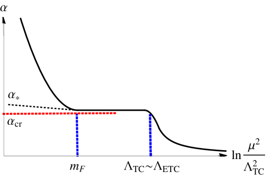
Note [11] that Eq.(2) has a multiple zero at $\alpha=\alpha_{\rm cr}\simeq\alpha_{*}$ (not linear zero) and is completely different from the two-loop beta function having the CBZ IR fixed point (having linear zero at $\alpha_{*}$) which is no longer valid in the broken phase $\alpha>\alpha_{*}\simeq\alpha_{\rm cr}$, where $\alpha(\mu)\searrow\alpha_{\rm cr}$ ($\mu\nearrow$). Then the would-be IR fixed point $\alpha_{*}\simeq\alpha_{\rm cr}$ is also regarded as the UV fixed point of the nonperturbative running (walking) coupling $\alpha(\mu)\approx\alpha_{\rm cr}$ [1] in the wide IR region $m_{F}<\mu<\Lambda=\Lambda_{\rm TC}$ for the characteristic large hierarchy $m_{F}\ll\Lambda_{\rm TC}$[39, 40]. (See also Ref.[41] for a similar observation.) See Fig. 1.¹²¹²12 Note also that the walking technicolor in the UV region $\mu^{2}>\Lambda_{\rm TC}^{2}$ must be changed into only a part of some larger picture, such as the Extended Technicolor (ETC)[42] or models having both technifermions and SM fermions as composites on the equal footing [43], to provide the mass to the SM fermions through communicating technifermion condensate to the SM fermions, so that discussing the walking technicolor in isolation does not make sense for $\mu^{2}>\Lambda_{\rm TC}^{2}$.

Now we come to our core result, ladder evaluation of the nonperturbative trace anomaly in the anti-Veneziano limit, which then yields the mass $M_{\phi}$ and decay constant $F_{\phi}$ of the technidilaton $\phi$ through PCDC [2] as in Eq.(15):[11, 40]

	$\displaystyle M_{\phi}^{2}F_{\phi}^{2}$	$\displaystyle=$	$\displaystyle-d_{\theta}\langle\theta_{\mu}^{\mu}\rangle=-\frac{\beta^{(\rm NP)}(\alpha(\mu^{2}))}{\alpha(\mu^{2})}\,\langle G_{\mu\nu}^{2}(\mu^{2})\rangle\simeq N_{C}N_{F}\frac{16}{\pi^{4}}m_{F}^{4}\quad\left(d_{\theta}=4\right)$		(25)
		$\displaystyle\simeq$	$\displaystyle 2.5\left[\frac{8}{N_{F}}\frac{4}{N_{C}}\right]v^{4}\,.\quad\left(v=246\,{\rm GeV}\right)$		(26)

Firstly, the rightmost value in Eq.(25) can be obtained by two different ladder calculations: one through direct evaluation of the vacuum energy by the effective potential at the stationary point (Solution of the SD equation, $\Sigma=\Sigma_{\rm sol}$)[44], $E=V_{\rm eff}(\Sigma=\Sigma_{\rm sol})=\langle\theta^{0}_{0}\rangle=(1/4)\langle\theta^{\mu}_{\mu}\rangle$, the other through the ladder evaluation of the trace anomaly [40, 11], i.e., the technigluon condensate $\langle G_{\mu\nu}^{2}\rangle$ times the nonperturbative beta function Eq.(2), both in precise agreement with each other. The agreement is in highly nontrivial manner, being independent of the renormalization point $\mu$ as it should be: $\langle G_{\mu\nu}^{2}(\mu^{2})\rangle\sim\ln^{3}(\mu^{2}/m_{F}^{2})$, while $\beta^{({\rm NP})}(\alpha(\mu^{2}))/\alpha(\mu^{2})\sim 1/\ln^{3}(\mu^{2}/m_{F}^{2})$, precisely cancelled by each other.[11]

Secondly, Eq.(26) is obtained by use of the Pagels-Stokar formula:

$$v^{2}=(246\,{\rm GeV})^{2}=N_{D}F_{\pi}^{2}\simeq N_{F}N_{C}\frac{1}{4\pi^{2}}\,m_{F}^{2}\simeq m_{F}^{2}\left[\frac{N_{F}}{8}\frac{N_{C}}{4}\right],$$

(27)

and the result indicates important $N_{F},N_{C}-$ dependence of $M_{\phi}^{2}F_{\phi}^{2}$ in the anti-Veneziano limit when $v=$ fixed[11]. Since the technidilaton is a flavor-singlet bound state, its decay constant by definition scales like $F_{\phi}^{2}\propto N_{F}N_{C}m_{F}^{2}(\propto v^{2})$ (Actually $F_{\phi}^{2}\simeq N_{F}N_{C}m_{F}^{2}$). Then $M_{\phi}^{2}/F_{\phi}^{2},M_{\phi}^{2}/v^{2}\sim 1/(N_{F}N_{C})\rightarrow 0$ in the anti-Veneziano limit, where the technidilaton becomes NG boson although no exact massless limit exists: the situation is in the same sense as the $\eta^{\prime}$ meson in the original Veneziano limit $N_{C}\rightarrow\infty$ with $N_{C}\alpha=$fixed, and $N_{F}/N_{C}\ll 1$.¹³¹³13 There exists no exact massless limit in the conformal phase transition at $\alpha=\alpha_{\rm cr}$, with $m_{F}=0$, where no massless spectrum exists (conformal phase), in sharp contrast to the Ginzburg-Landau phase transition where the spectrum continuously passes through the phase transition point with massless particles. [4]

Numerically, Eq.(26) implies that

$$F_{\phi}\simeq 5\,v\quad{\rm for}\,\,M_{\phi}\simeq\frac{v}{2}\simeq 125\,{\rm GeV}\quad\left(N_{F}=8,N_{C}=4\right)\,,$$

(28)

in the one-family model, which is best fit to the current LHC data of the 125 GeV Higgs. [12, 11] Similar results are also obtained in the holographic model for the walking technicolor.[13]

Now to the LHC phenomenology of the walking technicolor. Details are given in the talk by S. Matsuzaki in this meeting.[36] The model has in general a larger chiral symmetry $SU(N_{F})_{L}\times SU(N_{F})_{R}$ $(N_{F}>2)$ spontaneously broken by the technifermion condensate $\langle\bar{F}F\rangle\neq 0$, or the technifermion dynamical mass $m_{F}\neq 0$, down to the diagonal $SU(N_{F})_{V}$. Also spontaneously broken by the same technifermion condensate is the approximate scale symmetry due to the almost nonruning (walking) coupling $\alpha(\mu^{2})\approx\alpha_{\rm cr}$ in the wide infrared region $m_{F}^{2}<\mu^{2}<\Lambda_{\rm TC}^{2}$ ($m_{F}\ll\Lambda_{\rm TC}^{2}$). Moreover the scale symmetry is simultaneously broken explicitly by the same origin $m_{F}\neq 0$, an emergent infrared mass scale, resulting in the nonperturbative trace anomaly of dimension 4 operator as was given in Eq.(25).

The effective theory should have the same symmetry structure as the underlying theory. Namely, the nonlinear realization of both the chiral symmetry and the scale symmetry, which implies the scale-invariant nonlinear sigma model [12, 11]. Then the effective theory of the walking technicolor with $N_{F}$ massless flavors takes precisely the same scale-invariant form as the nonlinearly realized SM Higgs Lagrangian in Eq.(14), with $U=e^{i\pi^{a}\,T^{a}}$ being $N_{F}\times N_{F}$ unitary matrix (${\rm tr}\,T^{a}=0\,,{\rm tr}(T^{a}T^{b})=\delta^{ab}/2,\,a=1,\cdots,N_{F}^{2}-1$), except that the explicit scale breaking comes from the different potential $V^{(4)}(\phi)$ ¹⁴¹⁴14 This potential is indeed obtained by the explicit ladder computation of the effective potential at the conformal phase transition point: $V^{(4)}(\phi)=-(4N_{F}N_{C}m_{F}^{4}/\pi^{4})\chi^{4}(\ln\chi-1/4)$, in precise agreement with Eq.(29) through Eq.(25). See Eq.(65) in Ref. [4] responsible for the trace anomaly of dimension 4 operator this time: [12, 11]

	$\displaystyle{\cal L}_{\rm WTC}$	$\displaystyle=$	$\displaystyle\chi^{2}\cdot\left[\frac{1}{2}\left(\partial_{\mu}\phi\right)^{2}+\frac{F_{\pi}^{2}}{4}{\rm tr}\left({\cal D}_{\mu}U{\cal D}^{\mu}U^{\dagger}\right)\right]-V^{(4)}(\phi)-V^{(\rm SM)}(\phi)\,,$
	$\displaystyle V^{(4)}(\phi)$	$\displaystyle=$	$\displaystyle-\ln\chi\cdot\frac{\beta^{(\rm NP)}(\alpha)}{4\alpha}G_{\mu\nu}^{2}=\frac{M_{\phi}^{2}F_{\phi}^{2}}{4}\chi^{4}\left(\ln\chi-\frac{1}{4}\right)$
	$\displaystyle V^{(\rm SM)}(\phi)$	$\displaystyle=$	$\displaystyle-\chi^{2-\gamma_{m}}\left(m_{f}\chi\bar{f}f\right)-\ln\chi\left[\frac{\beta_{F}(\alpha_{s})}{4\alpha_{s}}{G^{({\rm gluon})}_{\mu\nu}}^{2}+\frac{\beta_{F}(\alpha_{e})}{4\alpha_{e}}{F^{({\gamma})}_{\mu\nu}}^{2}\right]\,,\,$
	$\displaystyle\chi$	$\displaystyle=$	$\displaystyle\exp\left(\frac{\phi}{F_{\phi}}\right)\,,$		(29)

where $F_{\phi}\neq F_{\pi}=v/\sqrt{N_{D}}=v/\sqrt{N_{F}/2}$ in general in contrast to the SM Higgs case $F_{\phi}=F_{\pi}=v$, the electroweak gauging was done as usual $\partial_{\mu}U\Rightarrow{\cal D}_{\mu}U=\partial_{\mu}U-ig_{2}W_{\mu}U+ig_{Y}UB_{\mu}$, and we have added $V^{(\rm SM)}(\phi)$, the scale symmetry breaking terms related to the SM particles arising from the technifermion contributions: mass term of the SM fermion $f$, (one loop) technifermion contributions to the trace anomaly for the gluon and photon operators, with $\beta_{F}(g_{s})=\frac{g_{s}^{3}}{(4\pi)^{2}}\frac{4}{3}N_{C}$ and $\beta_{F}(e)=\frac{e^{3}}{(4\pi)^{2}}\frac{16}{9}N_{C}$. It is obvious that ${\theta_{\mu}^{\mu}}^{({\rm TC})}=-\delta_{D}V^{(4)}(\phi)=\beta^{(\rm NP)}(\alpha)/(4\alpha)\cdot G_{\mu\nu}^{2}=-(M_{\phi}^{2}F_{\phi}^{2}/4)\chi^{4}$ up to total derivative, corresponding to the PCDC with $d_{\theta}=4$ ($\langle\chi\rangle=1$), Eq.(25).

References

- [1] K. Yamawaki, M. Bando and K. Matumoto, Phys. Rev. Lett. 56, 1335 (1986); M. Bando, T. Morozumi, H. So and K. Yamawaki, Phys. Rev. Lett. 59, 389 (1987).
- [2] M. Bando, K. Matumoto and K. Yamawaki, Phys. Lett. B 178, 308 (1986).
- [3] V. A. Miransky, Nuovo Cim. A 90 (1985), 149.
- [4] V. A. Miransky and K. Yamawaki, Phys. Rev. D 55, 5051 (1997); Errata, 56, 3768 (1997).
- [5] T. Maskawa and H. Nakajima, Prog. Theor. Phys. 52 (1974), 1326; 54 (1975), 860.
- [6] Y. Nambu, Superconductor Model of Elementary Particles and its Consequencies - Talk given at a conference at Purdue (1960); Y. Nambu and G. Jona-Lasinio, Phys. Rev. 122, 345 (1961).
- [7] S. Weinberg, Phys. Rev. D 13 (1976), 974; D 19 (1979), 1277; L. Susskind, Phys. Rev. D 20 (1979), 2619: See for a review of earlier literature, E. Farhi and L. Susskind, Phys. Rep. 74 (1981), 277.
- [8] C. N. Leung, S. T. Love and W. A. Bardeen, Nucl. Phys. B 273, 649 (1986).
- [9] B. Holdom, Phys. Rev. D 24, 1441 (1981).
- [10] T. Akiba and T. Yanagida, Phys. Lett. B 169 (1986), 432; T. W. Appelquist, D. Karabali and L. C. R. Wijewardhana, Phys. Rev. Lett. 57 (1986), 957; For an earlier work on this line see B. Holdom, Phys. Lett. B 150 (1985), 301.
- [11] S. Matsuzaki and K. Yamawaki, arXiv:1508.07688 [hep-ph], to be published in JHEP.
- [12] S. Matsuzaki and K. Yamawaki, Phys. Lett. B 719, 378 (2013); Phys. Rev. D 86, 035025 (2012); Phys. Rev. D 85, 095020 (2012).
- [13] S. Matsuzaki and K. Yamawaki, Phys. Rev. D 86, 115004 (2012).
- [14] S. Sakata, Prog. Theor. Phys. 16, 686 (1956).
- [15] M. Gell-Mann, Phys. Lett. 8, 214 (1964); G. Zweig, CERN-TH-401 (1964);PRINT-64-170 (1964).
- [16] Z. Maki, M. Nakagawa and S. Sakata, Prog. Theor. Phys. 28, 870 (1962).
- [17] M. Kobayashi and T. Maskawa, Prog. Theor. Phys. 49, 652 (1973).
- [18] H. S. Fukano, S. Matsuzaki, K. Terashi and K. Yamawaki, arXiv:1510.08184 [hep-ph].
- [19] M. Kurachi, S. Matsuzaki and K. Yamawaki, Phys. Rev. D 90, no. 5, 055028 (2014).
- [20] M. Bando, T. Kugo, S. Uehara, K. Yamawaki and T. Yanagida, Phys. Rev. Lett. 54 (1985), 1215; M. Bando, T. Kugo and K. Yamawaki, Nucl. Phys. B 259 (1985), 493.
- [21] M. Bando, T. Kugo and K. Yamawaki, Phys. Rept. 164 (1988), 217.
- [22] M. Harada and K. Yamawaki, Phys. Rept. 381, 1 (2003).
- [23] H. K. Lee, W. G. Paeng and M. Rho, arXiv:1504.00908 [nucl-th]; M. Rho, arXiv:1507.05173 [hep-ph], in this Proceedings; W. G. Paeng, T. T. S. Kuo, H. K. Lee and M. Rho, arXiv:1508.05210 [hep-ph].
- [24] S. Matsuzaki and K. Yamawaki, Phys. Rev. Lett. 113, no. 8, 082002 (2014)
- [25] V. A. Miransky, M. Tanabashi and K. Yamawaki, Phys. Lett. B 221, 177 (1989); Mod. Phys. Lett. A 4, 1043 (1989);
- [26] Y. Nambu, Chicago preprint EFI 89-08 (Feb., 1989). Earlier related discussions are given in H. Terazawa, K. Akama and Y. Chikashige, Phys. Rev. D 15, 480 (1977).
- [27] W. A. Bardeen, C. T. Hill and M. Lindner, Phys. Rev. D 41, 1647 (1990).
- [28] S. Shuto, M. Tanabashi and K. Yamawaki, in Proc. 1989 Workshop on Dynamical Symmetry Breaking, Dec. 21-23, 1989, Nagoya, eds. T. Muta and K. Yamawaki (Nagoya Univ., Nagoya, 1990) 115-123; M. S. Carena and C. E. M. Wagner, Phys. Lett. B 285, 277 (1992); M. Hashimoto, Phys. Lett. B 441, 389 (1998).
- [29] B. A. Dobrescu and C. T. Hill, Phys. Rev. Lett. 81, 2634 (1998); R. S. Chivukula, B. A. Dobrescu, H. Georgi and C. T. Hill, Phys. Rev. D 59, 075003 (1999)
- [30] H. S. Fukano, M. Kurachi, S. Matsuzaki and K. Yamawaki, Phys. Rev. D 90, no. 5, 055009 (2014); H. C. Cheng, B. A. Dobrescu and J. Gu, JHEP 1408, 095 (2014).
- [31] H. S. Fukano, arXiv:1507.08003 [hep-ph]. to appear in the SCGT15 Proceedings.
- [32] Y. Kikukawa and K. Yamawaki, Phys. Lett. B 234, 497 (1990).
- [33] K. i. Kondo, S. Shuto and K. Yamawaki, Mod. Phys. Lett. A 6, 3385 (1991); N. V. Krasnikov, Mod. Phys. Lett. A 8, 797 (1993); K. i. Kondo, M. Tanabashi and K. Yamawaki, Prog. Theor. Phys. 89, 1249 (1993); M. Harada, Y. Kikukawa, T. Kugo and H. Nakano, Prog. Theor. Phys. 92, 1161 (1994).
- [34] N. Arkani-Hamed, A. G. Cohen and H. Georgi, Phys. Rev. Lett. 86, 4757 (2001); C. T. Hill, S. Pokorski and J. Wang, Phys. Rev. D 64, 105005 (2001).
- [35] D. T. Son and M. A. Stephanov, Phys. Rev. D 69, 065020 (2004); T. Sakai and S. Sugimoto, Prog. Theor. Phys. 113, 843 (2005).
- [36] S. Matsuzaki, arXiv:1510.04575 [hep-ph], to be published in the SCGT15 Proceedings.
- [37] W. E. Caswell, Phys. Rev. Lett. 33, 244 (1974); T. Banks and A. Zaks, Nucl. Phys. B 196, 189 (1982).
- [38] T. Appelquist, J. Terning and L. C. Wijewardhana, Phys. Rev. Lett. 77, 1214 (1996) T. Appelquist, A. Ratnaweera, J. Terning and L. C. Wijewardhana, Phys. Rev. D 58, 105017 (1998).
- [39] K. Yamawaki, Prog. Theor. Phys. Suppl. 167, 127 (2007).
- [40] M. Hashimoto and K. Yamawaki, Phys. Rev. D 83, 015008 (2011).
- [41] D. B. Kaplan, J. W. Lee, D. T. Son and M. A. Stephanov, Phys. Rev. D 80, 125005 (2009).
- [42] S. Dimopoulos and L. Susskind, Nucl. Phys. B 155, 237 (1979); E. Eichten and K. D. Lane, Phys. Lett. B 90, 125 (1980).
- [43] K. Yamawaki and T. Yokota, Phys. Lett. B 113 (1982), 293; Nucl. Phys. B 223 (1983), 144.
- [44] V. P. Gusynin and V. A. Miransky, Phys. Lett. B 198, 79 (1987) [Ukr. Fiz. Zh. (Russ. Ed. ) 33, 485 (1988)].
- [45] S. Dimopoulos, Nucl. Phys. B 168, 69 (1980); E. Farhi and L. Susskind, Phys. Rept. 74, 277 (1981).
- [46] M. Kurachi, S. Matsuzaki and K. Yamawaki, Phys. Rev. D 90, no. 9, 095013 (2014), and references cited therein.
- [47] M. Kurachi, R. Shrock and K. Yamawaki, Phys. Rev. D 91, no. 5, 055032 (2015).
- [48] Y. Aoki, T. Aoyama, E. Bennett, M. Kurachi, T. Maskawa, K. Miura, K. -i. Nagai, H. Ohki and E. Rinaldi, A. Shibata, K. Yamawaki and T. Yamazaki (the LatKMI Collaboration), arXiv:1510.05863 [hep-lat]; arXiv:1510.07373 [hep-lat]. To be published in SCGT15 Proceedings.
- [49] Y. Aoki, T. Aoyama, M. Kurachi, T. Maskawa, K. -i. Nagai, H. Ohki, A. Shibata, K. Yamawaki and T. Yamazaki (the LatKMI Collaboration), Phys. Rev. D 86, 054506 (2012).
- [50] Y. Aoki, T. Aoyama, M. Kurachi, T. Maskawa, K. -i. Nagai, H. Ohki, A. Shibata, K. Yamawaki and T. Yamazaki (the LatKMI Collaboration), Phys. Rev. D 87, no. 9, 094511 (2013).
- [51] T. Appelquist et al. [LSD Collaboration], Phys. Rev. D 90, 114502 (2014); A. Hasenfratz, D. Schaich and A. Veernala, arXiv:1410.5886 [hep-lat].
- [52] Y. Aoki, T. Aoyama, M. Kurachi, T. Maskawa, K. -i. Nagai, H. Ohki and E. Rinaldi, A. Shibata, K. Yamawaki and T. Yamazaki (the LatKMI Collaboration), Phys. Rev. Lett. 111, no. 16, 162001 (2013).
- [53] Y. Aoki, T. Aoyama, M. Kurachi, T. Maskawa, K. Miura, K. -i. Nagai, H. Ohki and E. Rinaldi, A. Shibata, K. Yamawaki and T. Yamazaki (the LatKMI Collaboration), Phys. Rev. D 89, 111502(R) (2014); PoS LATTICE 2013 (2013) 070.
- [54] Z. Fodor, K. Holland, J. Kuti, D. Nogradi and C. H. Wong, PoS LATTICE 2013, 062 (2014); R. Brower, A. Hasenfratz, C. Rebbi, E. Weinberg and O. Witzel, arXiv:1411.3243 [hep-lat].
- [55] G. Aad et al. [ATLAS Collaboration], arXiv:1506.00962 [hep-ex]. See also V. Khachatryan et al. [CMS Collaboration], JHEP 1408, 173 (2014).
- [56] H. S. Fukano, M. Kurachi, S. Matsuzaki, K. Terashi and K. Yamawaki, Phys. Lett. B 750, 259 (2015).
- [57] H. S. Fukano, S. Matsuzaki and K. Yamawaki, arXiv:1507.03428 [hep-ph].