On A Class of Greedy Sparse Recovery Algorithms
Abstract
Sparse signal recovery deals with finding the sparest solution of an under-determined linear system . In this paper, we propose a novel greedy approach to addressing the challenges from such a problem. Such an approach is based on a characterization of solutions to the system, which allows us to work on the sparse recovery in the -space directly with a given measure. With -based measure, an orthogonal matching pursuit (OMP)-type algorithm is proposed, which significantly outperforms the classical OMP algorithm in terms of recovery accuracy while maintaining comparable computational complexity. An -based algorithm, denoted as , is derived. Such an algorithm significantly outperforms the classical basis pursuit (BP) algorithm. Combining with the CoSaMP-strategy for selecting atoms, a class of high performance greedy algorithms is also derived. Extensive numerical simulations on both synthetic and image data are carried out, with which the superior performance of our proposed algorithms is demonstrated in terms of sparse recovery accuracy and robustness against numerical instability of the system matrix and disturbance in the measurement .
Keywords: Sparse signal recovery; Greedy methods; Basis pursuit methods; Under-determined linear system; Low-rank interference; Compressed sensing.
1 Introduction
The sparse recovery problem, also known as the sparse linear inverse problem, has found extensive applications in many areas such as data science [1, 2], signal processing [3, 4, 5, 6], communications engineering [7, 8, 9], structural health monitoring [10, 11, 12], hyperspectral imaging [13, 14, 15], and deep learning [16, 17]. It plays a crucial role in the framework of compressed sensing (CS) [18, 19, 20, 21, 22, 23], and in deep learning for feature selection and designing efficient convolutional neural networks [24, 25, 26, 27, 28, 29].
Consider the following popularly used synthetic model:
| (1) |
where with , and is the representation of the measurement in . The associated sparse recovery problem regards for a given , finding such a solution of (1), denoted as , which has fewer nonzero entries than any other solution. Mathematically, it is formulated as
| (2) |
where , often denoted as norm though it is not a norm in a strict sense, represents the number of nonzero elements in a vector , that is - the cardinality of the support of a vector . A signal is said to be -sparse in if .
As is well known, the sparse recovery problem (2) is NP-hard and has been investigated for many years. Determining how to solve problem (2) efficiently and accurately is crucial for a wide range of sparsity-related problems. To the best of our knowledge, this remains an open problem, and there is still a significant need for more effective algorithms.
1.1 Related work
To accurately solve the sparse recovery problem (2), the very first question to raise is: when does it have a unique solution ? Let denote the smallest number of columns of that are linearly dependent. It is well known that the following result [30] plays a key role in sparse recovery: Let be any -sparse vector in , that is there exists a with such that . Then, problem (2) has one and only one solution, , if and only if satisfies
| (3) |
Let be the largest integer that is not bigger than . Then, any -sparse solution of is the unique solution of (2) as long as , which is assumed in the sequel.
Another very important concept is the restricted isometry property (RIP), introduced in [31], which is defined as follows: a matrix is said to satisfy the -RIP with if
| (4) |
where denotes the set of all -sparse signals in . It can be seen that if satisfies the -RIP, then any columns of are linearly independent, and hence condition (3) holds. Therefore, if with , then, the underdetermined system has a unique -sparse solution, which is .
As an NP-hard problem, (2) is not tractable due to the norm. To address this, a convex relaxation is commonly employed. In particular, two classes of methods are popularly used:
1.1.1 Iteratively re-weighted approaches
This class includes basis pursuit (BP)-based algorithms, which rely on replacing the norm with -minimization. This approach regularizes problem (2) with the following problem [32, 31]:
| (5) |
This is a convex problem and there exist standard algorithms designed to solve such a problem efficiently, particularly when the problem’s dimension is manageable. Denote as the algorithm implemented using MATLAB command linprog.m.
Note that ,where is the sign function. Thus, the -minimization-based BP approach mentioned above is just an approximation of , where is replaced with .
To further improve the sparse recovery accuracy of the BP-based approach, a better approximating function can be used, such as: where is a parameter used to regularize the singularity at . With this function, we define The corresponding sparse recovery problem is formulated as the following constrained minimization
This non-convex problem is then addressed with two classes of iteratively re-weighted algorithms [33, 34, 35, 36, 37, 38, 39]. These algorithms are based on a first-order approximation approach and can be unified as follows:
| (6) |
where is determined by the weighting scheme. For , the formulation (6) is referred to as the iteratively re-weighted BP (IRBP) [37, 38, 36], and for , it corresponds to the iteratively re-weighted least squares (IRLS) [35, 39, 33, 34].
In general, the weighting is determined by . For example, the th element of is given by
in [37], where was used for IRBP, while with for IRLS
used in [39].
The IRBP-based algorithms provide a powerful tool for solving sparse recovery problems. However, these algorithms are computationally demanding, especially for large-scale scenarios. To reduce computational complexity, an - minimization-based reformulation of (5) was proposed in [40, 41], and a class of iterative algorithms, including FISTA, was derived [42, 43].
The IRLS method is popularly used for non-smooth cost functions by solving a sequence of quadratic problems as specified in (6) with . The solution to the 1st equation of (6) is given by
| (7) |
Note that the algorithms (6) are -sensitive, and a time-varying is crucial for these algorithms to achieve state-of-the-art recovery performance. In [39], an -regularization strategy was proposed, where (6) with is iteratively run with a monotonically decreasing sequence . In this iterative procedure, - the solution given by (6) with , is used as the initial iterate for the next iteration. We denote such an iterative procedure as .
1.1.2 Greedy methods
By nature, sparse recovery aims to identify the support of the -sparse vector underlying the measurement . Thus, one sparse algorithm differs from another in how it detects the support. The iteratively re-weighted methods estimate the support through a global search in the -space and then select the indices of the largest entries in magnitude from their minimizer .
The greedy algorithms, as described in [44, 45], intends to address the sparse recovery problem (2) by solving the following alternative problem:
where is the given sparsity level. The non-zero entries of are identified sequentially through a procedure that minimizes residual. Such a method is known as the orthogonal matching pursuit (OMP) method.
The OMP algorithm extracts the indices one by one iteratively. The th atom, indexed by , is identified as follows:
| (8) |
Here, is the residual obtained at the th iteration:111Throughout this paper, we use MATLAB notations: denotes the th entry of a vector , while , and denote the th entry, the th column, and the th row of a matrix , respectively. Furthermore, let be a subset of . is defined as the sub-vector of the vector with dimension , obtained by excluding those entries whose indices do not belong to . where is the set of the indices detected before the th iteration and is the associated coefficient vector obtained in the th iteration.
1.2 Problem formulation and contribution
It should be pointed out that the iteratively re-weighted algorithms provide state-of-the-art sparse recovery performance. However, they are computationally demanding. In particular, IRLS-based algorithms, though much faster than the IRBP-based ones, can encounter numerical issues when the matrix is ill-conditioned (See (7)). By contrast, OMP is significantly more efficient. The most computationally demanding stage involves solving the least squares problem to update the non-zero entries. A class of iterative methods, such as gradient pursuit (GP) and conjugate gradient pursuit (CGP), can be used to address this issue, as described in [46]. To improve the recovery accuracy and update the index set of the non-zero entries more efficiently, one approach is to select multiple entries at once, rather than just one as in OMP. This leads to the development of stage-wise OMP (StOMP) [47], compressive sampling match pursuit (CoSaMP) [48], and stagewise weak GP (StWGP) [49]. A comprehensive survey of these issues as well as performance guarantees can be found in [50].
As well-known, the greedy methods can not yield a comparable sparse recovery performance to the iteratively re-weighted ones. Suppose that has its indices that all fall within the support . Then, , and this new system has a unique sparsest solution, denoted as , with . The -norm based minimization (8) can not ensure that the obtained index falls into because the cost function is a complicated function of the true indices to be detected and such a function changes with . This is the main reason why the OMP algorithm cannot generally yield a sparse recovery as accurate as the iteratively re-weighted algorithms, prompting the proposal of its variants such as CoSaMP and StOMP.
The question we ask ourselves: Can we transform the system into domain by characterizing its set of solutions and then work directly on the sparse recovery problem? If an estimate of is achieved, the next index can be selected as the one that corresponds to the largest entry in magnitude of this estimate. Intuitively, by doing so the accuracy of index detection can be improved. This motivates us to deal with the sparse recovery problem on the -space, instead of the measurement -space.
The main objective of this paper is to derive a class of greedy algorithms that operate directly in the -domain and outperform classical greedy algorithms (i.e., OMP, CoSaMP) in terms of sparse recovery accuracy while maintaining similar implementation complexity. Additionally, these algorithms offer greater robustness against the numerical instability caused by and interferences in the signal compared to the classical algorithms, especially the IRLS-based ones. Our contributions are summarized as follows.
-
•
Based on a characterization of solutions to equation (1), we propose a class of greedy sparse recovery approaches for a given sparsity measure. Such an approach allows us to work directly in the -space;
-
•
Two algorithms, denoted as and , are derived based on and , respectively. Despite having nearly the same computational complexity, significantly outperforms the classical OMP algorithm and is comparable to the classical BP algorithm in terms of recovery accuracy. Meanwhile, the algorithm significantly surpasses the classical OMP, BPC, and CoSaMP algorithms in terms of sparse recovery accuracy;
-
•
An improved version of has been derived, denoted as the algorithm, in which -minimization is used to enhance the sparsity. Fast variants of the algorithms and , denoted as and , are developed to accelerate and by selecting multiple atoms per iteration;
-
•
It is shown that the proposed algorithms such as , and their fast variants can be used to deal with low-rank interferences in the measurements effectively, which owes to the proposed characterization and is a significant advantage over the classical algorithms.
All claims have been validated through extensive numerical simulations on both synthetic and image data.
The paper is organized as follows. In Section 2, we derive a characterization of the solution set for the linear system . Based on this characterization, we propose a greedy approach to sparse recovery. Two specified algorithms, denoted as and , are presented in this section. Section 3 analyzes the performance of the proposed algorithms. An improved version of , denoted as , is derived in Section 4, where the -minimization is employed to enhance the sparsity. Fast variants of both and are also derived in this section. Numerical examples and simulations are presented in Section 5 to validate the theoretical results, evaluate the performance of the proposed methods, and compare them with some existing approaches. To end this paper, some concluding remarks are given in Section 6.
2 The Proposed Approach and Algorithms
Our proposed greedy approach is based on the following characterization of the solutions to the system (1).
Let be a singular value decomposition (SVD) of , where the diagonal matrix has dimension with . It then follows from that
Denote , , and . With , we can show that any solution to (1) is given by and hence is of the form , i.e.,
| (9) |
where . Consequently, the solution set of system (1) is completely characterized by the vector variable for a given . The sparse recovery problem (2) can then be converted into the following equivalent form222For simplicity, and are sometimes denoted as and , respectively, in the sequel.
| (10) |
The alternative formulation transforms the classical problem (2) from a constrained minimization to an unconstrained one, allowing us to directly address sparse recovery in the -space of dimension .
A traditional sparse recovery algorithm aims to find the -sparse solution for each measurement , where the system is parametrized by according to the model (1). In this paper, we propose a class of greedy algorithms that obtain the solution based on the proposed model (9), where the system is parametrized by . The input is computed as , serving as an initial estimate of . The parameters , which are equivalent to , are determined at the design stage. When deriving the algorithms, we assume that the triple is available, similar to in traditional methods.
2.1 The proposed greedy approach
Suppose that is a detected index, expected to be one of the elements in . Let’s consider how to detect the next index, say , in a greedy manner.
First of all, it follows from that the residual is given by or more simply , where , according to the proposed characterization (9), can be expressed as
where , as defined in (9).
Recall that . Together with and , we obtain
| (11) |
where . Define a set that is characterized by .
Remark 2.1.
It is important to note that since we assume has a unique -sparse vector , possesses the following properties:
-
•
having a unique -sparse element , if and only if and ;
-
•
, if .
Thus, any solution of
| (12) |
satisfies , and .
Assume that . We note that problem (12) with results in and . Then, the corresponding is the unique -sparse and the sparsest element in set . This fact implies that to detect the next index in , say , we can first identify the sparsest element in . Then, can be determined as the index corresponding to the largest entry in magnitude of .
It is based on this observation that we propose the following greedy method, whose th iteration involves
| (15) |
where with being the set of indices detected before, and its complement.333Throughout this paper, denotes a set of indices when is an integer, while, as defined before, denotes the support of a vector . Here, denotes the norm or one of its approximating measures.
Running (15) for iterations, the -sparse estimate of , denoted as , is given by . It will be shown in the next section that if , then , and which implies that the unique -sparse solution of has been obtained.
Although the norm is the best measure to deal with sparsity-related problems, one of its approximating measures has to be used, as the norm is NP-hard and hence not tractable. In the next two subsections, we will further elaborate on the proposed greedy approach (15) with two approximating measures.
2.2 An -relaxation
Now, consider , that is, the -relaxation of . Denote . We have
due to the fact that , where , as defined in (11), and . Then, the proposed greedy approach (15) turns to
| (17) |
as . We name the above approach , where the subscript “GL2” stands for greedy method with indices selected using minimization. We briefly denote the approach as , where , as mentioned before, is the initial estimate of .
We realize by noting that the proposed algorithm (17) is closely related to the classical OMP algorithm applied to the following higher dimensional system (than )
| (18) |
It can be seen that the algorithm differs from the classical OMP applied to (18) in how it detects the next index .
Remark 2.2.
It should be pointed out that, although the transformed system is theoretically equivalent to the original , the proposed algorithm significantly outperform the classical algorithm - the OMP algorithm applied directly to . The most important reason for this is the “residual” in the transformed system being , instead of the in the classical greedy approach. More details will be analyzed in the next section.
2.3 An -relaxation
Note that can be rewritten as , where
| (22) |
With , the proposed greedy approach (15) becomes
| (23) |
which is a greedy -based algorithm for sparse recovery.
As seen, such an iterative algorithm involves solving a series of -minimizations of the form
| (24) |
As shown in [31], the above problem can be converted as a linear programming problem and hence can be solved with one of the standard convex optimization techniques, such as the MATLAB command . For convenience, we denote the corresponding algorithm as : with the residual .
The outline of the proposed greedy -based algorithm (23), denoted as , is then presented in Algorithm 1. For convenience, we denote this algorithm as
Before proceeding to the next section, we first evaluate the performance of the proposed greedy algorithms through the following numerical experiment. We generate a sequence of samples with . Here, - a (column) -normalized matrix, and with are generated randomly. We run each of the four algorithms: , - the classical BP method, and , where with , for all the 1,000 samples .
Let denote the index set of the largest absolute entries of . A recovery of a -sparse is considered successful if the solution obtained by an algorithm satisfies The rate of successful recovery for an algorithm running samples is defined as , where is the number of successful recoveries out of the samples.
| 65.80% | 94.30% | 97.40% | 100% |
With the above setting, the successful recovery rates for the four algorithms are given in Table 1.
Let be an estimate of , both being -sparse. The signal-to-noise ratio of this estimation is defined as . When some of the nonzero entries of are very small, these entries have a little contribution to but it is very difficult to correctly identify the indices of these entries. In this paper, we consider a recovery to be successful if either all the indices of are detected or the corresponding exceeds 60 dB.
3 Performance Analysis of the Proposed Greedy Approach
From the numerical example presented above, we observe that the proposed algorithm significantly outperforms the classical and even surpasses . Meanwhile, as expected, the proposed achieves a perfect sparse recovery across all 1,000 samples. These results demonstrate that our proposed greedy approach successfully achieves the objective raised in Section 1.2. In this section, we conduct a detailed analysis of the proposed approach and the resulting algorithms.
3.1 Approach analysis
As understood, greedy methods, including our proposed approach (15), are designed based on minimizing a residual. Consequently, the generated sequence of residuals is non-increasing. Although the residuals converge, most greedy algorithms are expected to yield the unique solution within a finite number of iterations.
First of all, we present the following result associated with the proposed greedy approach (15).
Theorem 1.
Let denote the set of indices detected, and let be obtained using the proposed greedy approach (15). Furthermore, let be the residual, and denote as the vector satisfying
Then, when for , we have as long as .
Proof: First of all, we note that , that is which is equivalent to . It then follows from and that
We note that is -sparse when the condition given in the theorem holds and due to the assumption of uniqueness on . Thus, is of full (column) rank, and hence the above equation leads to . This completes the proof.
In fact, the claims in Theorem 1 also hold for the classical algorithm, in which the upper bound for the number of iterations is set to . This means that must select an index that falls within , which precludes the possibility of making some mistakes in selecting indices. However, these mistakes can be rectified by taking more than iterations [50]. In general, for with , nothing can guarantee whether holds unless is verified.
The primary advantage of the proposed greedy approach over classical methods, such as and CoSaMP, lies in its index selection strategy. In the proposed greedy approach (15), the next index is chosen as the one corresponding to the largest absolute entry of the residual . As demonstrated in Remark 2.1 and the surrounding discussion, this selection ensures that belongs to . In contrast, determines by minimizing with respect to for . However, such a selection does not necessarily guarantee that belongs to , even if , as the minimizer of may not correspond to an index within .
Furthermore, let be the detected indices and be a subset of , which contains elements with . Using similar arguments to those in Remark 2.1, we have
for which the residual is
as long as holds, where and otherwise, . This implies that with taking , the index of the absolutely largest entry of the residual should fall within , provided that more than half of the detected indices belong to . In other words, when the first few indices are detected correctly, the proposed greed approach tolerates a small number of mistakes in index detection. This is indeed a remarkable property.
Remark 3.1.
The conclusion drawn above is based on the use of the ideal sparsity measure . Intuitively, the same conclusion is likely to hold with a high probability when a good approximating measure of is used. Indeed, the excellent performance of , in which is used, appears to support this argument. This highlighted property suggests that algorithms yielding better performance than could be developed by using the proposed greedy approach with more suitable approximating measures of . This will be elaborated further in the next section.
3.2 Comparison between and
As argued above, the key to outperforming the classical algorithm lies in its method of detecting the support . Another contributing factor is related to the numerical properties of the system matrix, including the concept of spark and RIP (see equations (3) (4)), and mutual coherence. In fact, let with . It was shown in [30] and [45] that both the classical and algorithms can yield the true solution from the system with (column) -normalized, if the following condition holds:
| (25) |
where is the mutual coherence of . As shown in [51], for a matrix with , and the lower bound is achieved if and only if the Gram matrix satisfies . Such a is called an equiangular tight-frame (ETF).
The condition (25) is just a sufficient condition to ensure a prefect recovery of . As shown in [52] and [53], the spare recovery accuracy of is more closely related to averaged mutual coherence of , denoted as , which is defined as the mean of all the squared off-diagonal entries of rather than . This implies that it is desired for the system matrix to have its Gram matrix close to the identity matrix . Based on this argument, it was shown in [53] and [54] that an optimal is a tight-frame (TF), whose Gram matrix is of form where is orthonormal. As ETFs exist only for some pairs , tight-frames provide an alternative for designing sparse recovery systems [55, 56, 57].
Our proposed algorithm is based on the system . As shown in (11), . We note that
-
•
It is difficult to find an explicit relationship between and . However, is actually a 1-tight frame and extensive examples have shown that ;
-
•
The classical algorithm intends to find such that the residual goes to nil as much as possible. Clearly, . Assume that is uncorrelated with a zero-mean. Thus, is diagonal with , where denotes the statistical average operation. Then, is given by , as is (column) -normalized.
Applying the above to the higher-dimensional system , we obtain Since , we can see that . This implies that, in a statistical sense, converges faster than ;
-
•
Let be a matrix with the -RIP property. It follows from that
where and are the smallest and largest (nonzero) singular values of , respectively. It can be shown that with some manipulations that satisfies the -RIP property with If is well-conditioned,444This is usually a necessary condition for the sparsifying systems to function properly. i.e., the condition number is not far away from one, so is . Thus, most of the theoretical results for the original system hold for the transformed system .
Now, let us consider the implementation complexity of . Define It follows from (9) and that the 1st equation of (17) can be rewritten as
Comparing to its counterpart in : , we can see that at the stage of obtaining the optimal coefficients, our proposed has exactly the same computation complexity if is available. We note that the extra computational burden, denoted as , for computing involves multiplications and additions.
Regarding the index selection stage, i.e., the 2nd equation of (17), our proposed algorithm needs to compute the residual as follows
while requires computing with
This implies that both algorithms have the same computational complexity at this stage.
Therefore, we claim that our proposed algorithm significantly outperforms , albeit at the price of an extra computational burden .555Note that converting the original system into the higher dimensional system requires the SVD of . Since this regards designing the system/algorithm and is done once only, the computational complexity involved at this stage is not considered part of the algorithm’s overall complexity.
3.3 Comparison between and
Recall that refers to the BP algorithm based on the classical formulation (5), while denotes the BP algorithm based on the reformulation (24) of (5). They are mathematically equivalent.
Compared to , the two BP-based algorithms adopt a global optimization approach to detect . However, the interactions among the entries in , imposed by the constraint , make it challenging to identify the sparsest solution . The proposed algorithm is specifically designed to mitigate the influence of the magnitudes of detected atoms on the identification of subsequent indices in a greedy manner. It leverages the strengths of both the classical and algorithms, effectively combining their advantages. Consequently, the substantial performance improvement over , as previously discussed, primarily stems from the method used to detect the support , which is performed in a higher-dimensional space.
The proposed algorithm exhibits excellent performance in terms of sparse recovery accuracy. Regarding implementation complexity, however, it requires solving -minimization problems of the form , i.e., (24), using . Consequently, similar to and , both of which are implemented via linear programming, is computationally demanding.
More efficient algorithms for solving (24) are needed to enable the use of in large-scale sparse recovery systems. Indeed, a subgradient-based algorithm was proposed in [58] for solving (24), which significantly outperforms in terms of speed and has substantially lower implementation complexity. In the next section, we introduce an IRLS-based algorithm for solving (24). By replacing with this IRLS-based approach in , the resulting algorithm not only achieves significantly faster convergence but also delivers superior sparse recovery performance.
4 Improved Algorithms
The proposed algorithm is computationally slow due to two main factors: i) it relies on linear programming-based BP; and ii) similar to the classical OMP, it selects atoms one-by-one. Additionally, the proposed algorithm is designed to solve the minimization problems of the form (15) with defined as the -norm. Higher performance algorithms can be developed by employing a more effective norm to approximate the sparsity norm .
In this section, we derive a class of efficient algorithms that adopt an atom update scheme similar to that of CoSaMP and explore strategies for handling cases where the measurements are contaminated by noise.
4.1 Iteratively re-weighted approach to (15)
Note that the cost function of (15) is of form
| (29) |
where represents an approximating function of the sign function .
Thus, the key to (15) is to solve
| (30) |
Here, we consider two approximating functions defined before: where and . When represents , (30) is convex and can be solved using , resulting in the algorithm.
When represents the -norm , is highly non-convex and such a problem can be addressed using the IRLS method, which generates a sequence for a fixed in the way:
| (31) |
where and , with the diagonal given by
| (32) |
Note that the solution to the 1st term of (31) is given by
| (33) |
We use the same -regularization scheme to set and the stopping criterion as in [39]. The corresponding -regularized IRLS algorithm, denoted as to differentiate the classical , is presented in Algorithm 2. For convenience, we denote this algorithm as As understood, with replaced by in a similar algorithm to can be obtained. Such an algorithm is denoted as .
Remark 4.1.
It should be noted that the solution to (31) is theoretically obtained through matrix inversion as shown in (33). However, this solution for the unconstrained LS problem can also be computed using more efficient iterative algorithms, such as GP and CGP, which avoid matrix inversion. See [46] for details. This provides a significant advantage of our proposed over the classical , which requires a large number of matrix inversions (see (7)). These inversions are not only computationally expensive but can also lead to numerical issues when the system matrix is ill-conditioned. This advantage will be further demonstrated in the simulation section.
4.2 CoSaMP-type algorithms for sparse recovery
As mentioned earlier, although achieves excellent sparse recovery performance, it is very slow, partially due to the one-by-one update of atoms. By using the same idea as in CoSaMP, we can update the set of selected atoms with multiple atoms at each iteration.
Let be an algorithm, say or , derived earlier. Its improved version, which uses a CoSaMP-type strategy for updating the set of selected indices, is denoted as and outlined in Algorithm 3 (for ). For convenience, we denote this algorithm as By replacing with in , we obtain .
Remark 4.2.
We note that (i) the parameter is determined by the sparse recovery performance of the associated algorithm, like and . In general, is chosen such that ; (ii) as observed, the number of indices selected in is equal to , except during the first iteration, where indices are included. This number can be slightly greater than but is definitely smaller than . See Theorem 1.
4.3 Robust sparse recovery algorithms against low-rank disturbance
So far, our discussion has been limited to the case where the measurement signal is strictly sparse. Now, we consider a more practical scenario where the signal is of the following form
| (34) |
where represents a disturbance that affects the recovery of the true sparse vector from .
The objective here is to separate and from a given. A traditional approach to address this problem is to first obtain a primary estimate of the true underlying by applying a sparse recovery algorithm to . Then, defining as the set of indices corresponding to the largest entries of in magnitude, an estimate of the clean is given by
| (35) |
where is -sparse and satisfies , with This estimation procedure corresponds to the classical Oracle estimator [31] when . In general, the classical sparse recovery algorithms are highly sensitive to noise . Even when , the obtained estimate does not necessarily equal unless .
There are scenarios, in which is often modeled as a low-rank signal [59, 60]:
| (36) |
where with is a matrix satisfying , and is an unknown vector. In multiple measurement vector models, (34) transforms into a low-rank and sparse decomposition problem, a framework that has been extensively studied in the literature [61, 62, 63, 64, 65]. Similar to the Robust PCA (RPCA)-based approach introduced in [61], most of these works focus on the special case where , investigating various methods for separating the low-rank and sparse components. In this paper, we address the problem of recovering the clean signal from as given in (34), with modeled by (36). We consider the scenario where both and are known, with having dimensions and assuming .
Note . Under our proposed characterization, we have , and hence
Based on this formulation, we propose the following robust approach to sparse recovery
| (37) |
Let . It was shown in [58] that (37) has a unique -solution if and only if all the submatrices of are of rank , which holds when . Since, in general, , ensuring this condition requires that , which simplifies to
As observed, (37) has the same form as (10). Consequently, it can be addressed using classical methods such as and the just derived . More interestingly, with replaced by , our proposed greedy algorithms such as , , and , can also be applied to solve (37).
Remark 4.3.
It is important to highlight the following key points:
-
•
The results obtained above indicate that the true support can be recovered with high probability using our proposed algorithms, even in the presence of disturbance . This demonstrates a significant advantage of our proposed sparse model over the classical formulation ;
-
•
Let be the primary estimate of obtained using one of our proposed algorithms. Suppose that - the set of indices corresponding to the largest entries of , is equal to . In this case, the estimate can be computed using the classical Oracle estimator (35). Alternatively, it follows from and that Thus, we have
where . The corresponding estimate of is given by This result implies that the clean signal can be exactly recovered using the framework based on our proposed model or characterization, provided that ;
-
•
Note . The sparsity-based signal separation problem can then be formulated as the classical form:
where . However, solving this problem using classical algorithms such and is challenging due to the potential numerical ill-conditioning of . In particular, can not be directly applied to the problem due to the singularity of . Furthermore, even if the true support is correctly identified using a classical algorithm, the clean signal cannot be recovered using the classical Oracle estimator, as previously discussed.
5 Numerical examples and simulations
In this section, we present a number of numerical examples and simulations in MATLAB to demonstrate the performance of five classical algorithms and five proposed algorithms:
- •
-
•
- the classical compressive sampling match pursuit (CoSaMP) algorithm [48];
- •
-
•
- the iteratively re-weighted least squares (IRLS) algorithm proposed in [39] with ;
-
•
FISTA - the fast iterative shrinkage-thresholding (FISTA) algorithm proposed in [42];
-
•
- the proposed greedy algorithm using ;
-
•
- the proposed greedy algorithm with atoms selected one-by-one using ;
-
•
- the proposed fast greedy algorithm with atoms selected at each iteration using ;
-
•
- the proposed greedy algorithm with atoms selected one-by-one using ;
-
•
- the proposed fast greedy algorithm with atoms selected at each iteration using .
5.1 Data setting and measures
The synthetic data used in this section is generated as follows: For a given setting , we create a matrix of dimension using randn, and the system matrix is obtained by normalizing the columns of this matrix. A sequence of -sparse samples, , is generated with the positions of the non-zero entries randomly selected using randperm, while these entries are produced using randn such that .
To evaluate the performance of a sparse recovery algorithm, we adopt the rate of successful sparse recovery and the signal-to-noise ratio (SNR), both defined at the end of Section 2. Furthermore, the wall-clock time in seconds, denoted as , represents the total time taken by an algorithm to process the samples.
5.2 Sparse recovery accuracy and computational efficiency
| FISTA | |||||||||||
|---|---|---|---|---|---|---|---|---|---|---|---|
| 99% | 100% | 100% | 100% | 99% | 100% | 100% | 100% | 100% | 100% | ||
| 3.05e-2 | 2.09e-2 | 8.43e-1 | 3.20e-1 | 4.04e-1 | 2.22e-2 | 2.00e+0 | 2.00e+0 | 2.26e-1 | 2.06e-1 | ||
| 6% | 0% | 11% | 92% | 3% | 53% | 94% | 78% | 99% | 94% | ||
| 2.12e-1 | 9.87e+0 | 1.12e+0 | 1.05e+0 | 2.75e+0 | 2.27e-1 | 3.02e+1 | 7.34e+0 | 6.31e+0 | 1.87e+0 | ||
| 85% | 100% | 100% | 100% | 62% | 100% | 100% | 100% | 100% | 100% | ||
| 3.88e-1 | 1.76e-1 | 4.71e+0 | 2.84e+0 | 1.91e+1 | 5.40e-1 | 1.47e+1 | 1.47e+1 | 2.32e+0 | 2.29e+0 | ||
| 8% | 0% | 4% | 100% | 0% | 56% | 100% | 99% | 100% | 100% | ||
| 1.62e+0 | 8.14e+1 | 5.99e+0 | 5.24e+0 | 2.07e+1 | 2.38e+0 | 3.02e+2 | 3.58e+1 | 3.92e+0 | 3.81e+0 | ||
| 90% | 100% | 100% | 100% | 35% | 100% | 100% | 100% | 100% | 100% | ||
| 2.68e+0 | 7.78e-1 | 3.13e+1 | 9.07e+0 | 5.55 e+1 | 3.69e+0 | 1.18e+2 | 1.18e+2 | 6.93e+0 | 6.77e+0 | ||
| 16% | 0% | 53% | 100% | 0% | 90% | 100% | 100% | 100% | 100% | ||
| 9.05e+0 | 2.82e+2 | 4.63e+1 | 1.44e+1 | 5.90e+1 | 1.09e+1 | 1.03e+3 | 2.05e+2 | 1.04e+1 | 1.04e+1 |
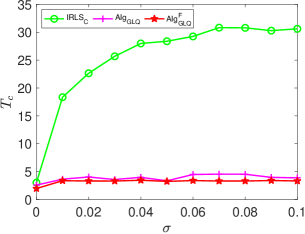
Table 2 shows the performance of the ten algorithms for different settings with samples. The ten algorithms are further evaluated under the setting and , with varying from 4 to in steps of 4. Fig. 1 shows the corresponding statistics of and . We note from the simulations above that 1) among the five classical algorithms, achieves the best sparse recovery performance and is significantly faster than ; 2) the proposed achieves the same sparse recovery accuracy as when is small, but with much higher computational efficiency; 3) the other four proposed algorithms, i.e., , , , and , demonstrate a similar performance to . Notably, , and even outperform the state-of-the-art algorithm in terms of .
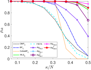
(a)
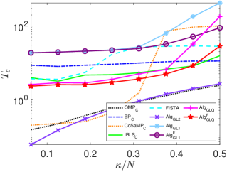
(b)
As observed in Table 2, the classical algorithms , and FISTA, along with the proposed and , become very time-consuming as the dimension of the system (matrix) gets large. Therefore, in the sequel, we will focus on the other five algorithms when large-scale systems are concerned. Fig. 2 presents simulations similar to those in Fig. 1 for the five algorithms: , , , and , under the setting and , with ranging from 64 to 144 in steps of 8. As observed, the proposed algorithms and can perfectly reconstruct all samples, similar to the performance of the algorithm, when is small (e.g., ), but with much higher computational efficiency. However, as increases, the proposed and algorithms demonstrate superior sparse recovery performance, albeit with higher computational time requirements.
(a)
(b)
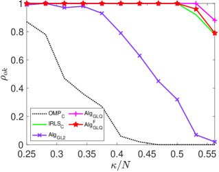
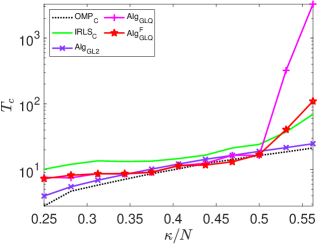
To investigate the impact of sparsity level and signal dimension on the performance of the five algorithms: , , , and , we repeat the above experiments with samples and generate phase transition plots, as shown in Fig. 3. These experiments span signal dimensions and sparsity levels . The results demonstrate that the proposed algorithm significantly outperforms the other four algorithms in terms of successful recovery rates. In addition, its accelerated version, , achieves a slightly higher successful recovery rate compared to , as shown in Fig. 3 (f), which highlights the differences in successful recovery rates between and .
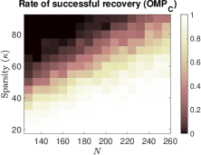
(a)
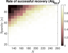
(b)
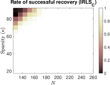
(c)
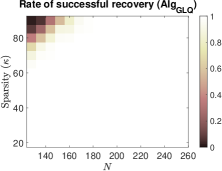
(d)
(e)
(f)
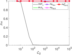
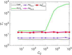
5.2.1 Effects of system matrix conditioning
From the above, we note that the classical and our proposed and yield almost identical performance for those systems generated using and subsequently normalized. These matrices are well-conditioned. We note from (7), may encounter numerical issues when is ill-conditioned.
Let denote the condition number of , where and are the biggest and smallest of singular values of . For a given pair , we can generate a system matrix in the same way as used in [66] for a specified . We now consider the following settings: (i) and ; and (ii) and . Fig.s 4 and 5 depict the statistics for and under each setting, respectively, where the system matrices are generated with varies within
(a)
(b)
(a)
(b)
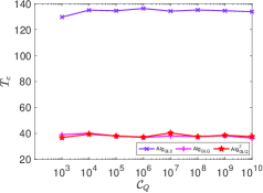
It is observed that the of the classical is very sensitive to . This is not the case for our proposed . Furthermore, 1) the of increases dramatically when exceeds , reaching values hundreds of times greater than those of and . Indeed, when exceeds , encounters numerical issues and fails to work properly; 2) the conditioning number has almost no effect on the performance of the three of our proposed algorithms in terms of and . This is further confirmed under the setting and , where varies from . For all the proposed three algorithms, is constantly equal to one, while the Wall-clock time is presented in Fig. 6.
In summary,
-
•
for well-conditioned systems, our proposed algorithms , and achieve the same or even better sparse recovery performance compared to the state-of-art performance algorithm . Additionally, the proposed significantly outperforms the classical and in terms of sparse recovery, with computational efficiency comparable to ;
-
•
for ill-conditioned systems, the performance of all classical algorithms degrades dramatically in terms of either sparse recovery accuracy or computational efficiency, or both. In contrast, the three proposed algorithms , and can work properly even for systems with up to and large-scale dimensions.
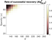
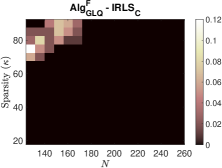
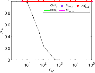
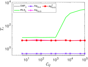
5.3 Robustness against low-rank disturbance
Next, we evaluate the performance of our proposed algorithms under the noisy signal model introduced in Section 4.3, with a particular focus on comparing them to .
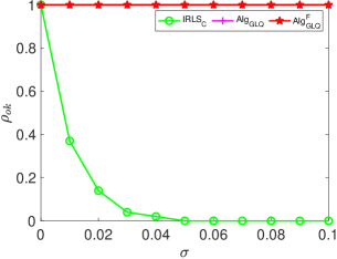
5.3.1 Synthetic data
We repeat the previous experiments with parameters , and . We set and construct using the first left singular vectors of an Gaussian random matrix with entries drawn from . The coefficient in (36) is then generated as , where is a normalized Gaussian random vector with entries following . Here, our primary focus is on comparing the performance of our proposed and algorithms against . As illustrated in Fig. 7, our proposed methods demonstrate significant advantages over algorithm in terms of both successful recovery rate and computational efficiency. Notably, as the noise level increases to , completely fails to reconstruct the signals, whereas the proposed and maintain perfect recovery performance across all the signals.
(a)
(b)
5.3.2 Image transmission
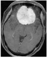
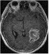
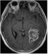
We consider an image transmission system affected by a low-rank interference signal modeled as in (36), with assumed to be known. The clean images intended for transmission are shown in the first column of Fig. 8. Prior to transmission, each clean image is divided into patches of size , resulting in an data matrix with and corresponding to the number of patches. After transmission, the received noisy images are presented in the second column of Fig. 8.
Given the noisy images, we reconstruct the clean images using six different algorithms: , , , , , and . In the reconstruction process, we employ an overcomplete discrete cosine transform (DCT) dictionary of size , i.e., . The sparsity level is set differently for each image, with specific values provided in Table 3. The corresponding image sizes are also listed in Table 3. The reconstructed images obtained from the six algorithms are displayed in Fig. 8. Table 3 further presents the peak signal-to-noise ratio (PSNR, in dB) for each method. The results demonstrate that our four proposed algorithms achieve significantly higher PSNR values compared to and , highlighting their superior performance in reconstructing the clean images.
Clean

MRI1
Noisy


MRI2


| Size | Noisy | ||||||||
|---|---|---|---|---|---|---|---|---|---|
| MRI1 | 20 | 24.42 | 25.03 | 25.13 | 50.45 | 49.72 | 49.94 | 49.90 | |
| MRI2 | 12 | 20.47 | 22.05 | 22.22 | 55.22 | 55.01 | 55.01 | 54.83 |
6 Concluding remarks
In this paper, we have investigated the sparse signal recovery problems. Our study has led to several key findings and contributions that enhance the field of sparse signal recovery. Based on a proposed system model, we have developed a novel approach leading to a class of greedy algorithms, including
-
•
three innovative greedy algorithms, , and , which significantly improve the accuracy of classical methods such as OMP and BP;
-
•
two fast algorithms, and , designed to accelerate and , achieving performance that even surpasses state-of-the-art sparse recovery methods.
Furthermore, the five proposed algorithms demonstrate excellent robustness against instability caused by the poor numerical properties of the system matrix and measurement interferences – issues that significantly affect classical sparse recovery algorithms.
Future work will focus on further enhancing the algorithms’ efficiency and exploring their applications in more complex high-dimensional data analysis tasks, such as hyperspectral imaging, seismic data processing, and wireless communication. In conclusion, the proposed greedy algorithms represent a significant advancement in sparse recovery techniques. By combining theoretical rigor with practical efficiency, our work paves the way for future innovations and applications in the field of signal processing and beyond.
References
- [1] Vladimir Shikhman, David Müller, Vladimir Shikhman, and David Müller. Sparse recovery. Mathematical Foundations of Big Data Analytics, pages 131–148, 2021.
- [2] Stanley Osher. Sparse recovery for scientific data. Technical report, Univ. of California, Los Angeles, CA (United States), 2019.
- [3] Ljubiša Stanković, Ervin Sejdić, Srdjan Stanković, Miloš Daković, and Irena Orović. A tutorial on sparse signal reconstruction and its applications in signal processing. Circuits, Systems, and Signal Processing, 38:1206–1263, 2019.
- [4] Shuang Li, Michael B Wakin, and Gongguo Tang. Atomic norm denoising for complex exponentials with unknown waveform modulations. IEEE Transactions on Information Theory, 66(6):3893–3913, 2019.
- [5] Mike E Davies and Yonina C Eldar. Rank awareness in joint sparse recovery. IEEE Transactions on Information Theory, 58(2):1135–1146, 2012.
- [6] Natalie Durgin, Rachel Grotheer, Chenxi Huang, Shuang Li, Anna Ma, Deanna Needell, and Jing Qin. Jointly sparse signal recovery with prior info. In 2019 53rd Asilomar Conference on Signals, Systems, and Computers, pages 645–649. IEEE, 2019.
- [7] Yuzhe Jin, Young-Han Kim, and Bhaskar D Rao. Limits on support recovery of sparse signals via multiple-access communication techniques. IEEE Transactions on Information Theory, 57(12):7877–7892, 2011.
- [8] Xing Zhang, Haiyang Zhang, and Yonina C. Eldar. Near-field sparse channel representation and estimation in 6G wireless communications. IEEE Transactions on Communications, 72(1):450–464, 2023.
- [9] Shuang Li, Daniel Gaydos, Payam Nayeri, and Michael B Wakin. Adaptive interference cancellation using atomic norm minimization and denoising. IEEE Antennas and Wireless Propagation Letters, 19(12):2349–2353, 2020.
- [10] Yong Huang, James L Beck, Stephen Wu, and Hui Li. Bayesian compressive sensing for approximately sparse signals and application to structural health monitoring signals for data loss recovery. Probabilistic Engineering Mechanics, 46:62–79, 2016.
- [11] Shuang Li, Dehui Yang, Gongguo Tang, and Michael B Wakin. Atomic norm minimization for modal analysis from random and compressed samples. IEEE Transactions on Signal Processing, 66(7):1817–1831, 2018.
- [12] Zhiyi Tang, Yuequan Bao, and Hui Li. Group sparsity-aware convolutional neural network for continuous missing data recovery of structural health monitoring. Structural Health Monitoring, 20(4):1738–1759, 2021.
- [13] Mohammad Golbabaee and Pierre Vandergheynst. Hyperspectral image compressed sensing via low-rank and joint-sparse matrix recovery. In 2012 IEEE International Conference on Acoustics, Speech and Signal Processing (ICASSP), pages 2741–2744. IEEE, 2012.
- [14] Boaz Arad and Ohad Ben-Shahar. Sparse recovery of hyperspectral signal from natural RGB images. In Computer Vision–ECCV 2016: 14th European Conference, Amsterdam, The Netherlands, October 11–14, 2016, Proceedings, Part VII 14, pages 19–34. Springer, 2016.
- [15] Natalie Durgin, Rachel Grotheer, Chenxi Huang, Shuang Li, Anna Ma, Deanna Needell, and Jing Qin. Fast hyperspectral diffuse optical imaging method with joint sparsity. In 2019 41st Annual International Conference of the IEEE Engineering in Medicine and Biology Society (EMBC), pages 4758–4761. IEEE, 2019.
- [16] Yann LeCun, Yoshua Bengio, and Geoffrey Hinton. Deep learning. Nature, 521(7553):436–444, 2015.
- [17] Ian Goodfellow, Yoshua Bengio, and Aaron Courville. Deep Learning. MIT press, 2016.
- [18] David L Donoho. Compressed sensing. IEEE Transactions on Information Theory, 52(4):1289–1306, 2006.
- [19] Emmanuel J Candès and Michael B Wakin. An introduction to compressive sampling. IEEE Signal Processing Magazine, 25(2):21–30, 2008.
- [20] Marco F Duarte and Yonina C Eldar. Structured compressed sensing: From theory to applications. IEEE Transactions on Signal Processing, 59(9):4053–4085, 2011.
- [21] Zhihui Zhu, Gang Li, Jiajun Ding, Qiuwei Li, and Xiongxiong He. On collaborative compressive sensing systems: The framework, design, and algorithm. SIAM Journal on Imaging Sciences, 11(2):1717–1758, 2018.
- [22] Roman Vershynin, Y. C. Eldar, and Gitta Kutyniok. Introduction to the non-asymptotic analysis of random matrices. In Y. C. Eldar and G. Kutyniok, editors, Compressed Sensing: Theory and Applications. Cambridge University Press, UK, 2012.
- [23] Simon Foucart and Holger Rauhut. A Mathematical Introduction to Compressive Sensing. Birkhäuser New York, NY, 2013.
- [24] Jie Gui, Zhenan Sun, Shuiwang Ji, Dacheng Tao, and Tieniu Tan. Feature selection based on structured sparsity: A comprehensive study. IEEE Transactions on Neural Networks and Learning Systems, 28(7):1490–1507, 2016.
- [25] Shiyun Xu, Zhiqi Bu, Pratik Chaudhari, and Ian J Barnett. Sparse neural additive model: Interpretable deep learning with feature selection via group sparsity. In Joint European Conference on Machine Learning and Knowledge Discovery in Databases, pages 343–359. Springer, 2023.
- [26] Alex Krizhevsky, Ilya Sutskever, and Geoffrey E Hinton. Imagenet classification with deep convolutional neural networks. Advances in Neural Information Processing Systems, 25, 2012.
- [27] Baoyuan Liu, Min Wang, Hassan Foroosh, Marshall Tappen, and Marianna Pensky. Sparse convolutional neural networks. In Proceedings of the IEEE Conference on Computer Vision and Pattern Recognition, pages 806–814, 2015.
- [28] Jerome Friedman, Trevor Hastie, and Rob Tibshirani. Regularization paths for generalized linear models via coordinate descent. Journal of Statistical Software, 33(1):1, 2010.
- [29] Zhonghua Liu, Zhihui Lai, Weihua Ou, Kaibing Zhang, and Ruijuan Zheng. Structured optimal graph based sparse feature extraction for semi-supervised learning. Signal Processing, 170:107456, 2020.
- [30] David L Donoho and Michael Elad. Optimally sparse representation in general (nonorthogonal) dictionaries via minimization. Proceedings of the National Academy of Sciences, 100(5):2197–2202, 2003.
- [31] Emmanuel J Candès and Terence Tao. Decoding by linear programming. IEEE Transactions on Information Theory, 51(12):4203–4215, 2005.
- [32] Scott Shaobing Chen, David L Donoho, and Michael A Saunders. Atomic decomposition by basis pursuit. SIAM Review, 43(1):129–159, 2001.
- [33] Irina F Gorodnitsky and Bhaskar D Rao. Sparse signal reconstruction from limited data using FOCUSS: A re-weighted minimum norm algorithm. IEEE Transactions on Signal Processing, 45(3):600–616, 1997.
- [34] Bhaskar D Rao and Kenneth Kreutz-Delgado. An affine scaling methodology for best basis selection. IEEE Transactions on Signal Processing, 47(1):187–200, 1999.
- [35] Ingrid Daubechies, Ronald DeVore, Massimo Fornasier, and C Sinan Güntürk. Iteratively reweighted least squares minimization for sparse recovery. Communications on Pure and Applied Mathematics: A Journal Issued by the Courant Institute of Mathematical Sciences, 63(1):1–38, 2010.
- [36] Xiaolin Huang, Yipeng Liu, Lei Shi, Sabine Van Huffel, and Johan AK Suykens. Two-level minimization for compressed sensing. Signal Processing, 108:459–475, 2015.
- [37] Emmanuel J Candes, Michael B Wakin, and Stephen P Boyd. Enhancing sparsity by reweighted minimization. Journal of Fourier Analysis and Applications, 14:877–905, 2008.
- [38] Yilun Wang and Wotao Yin. Sparse signal reconstruction via iterative support detection. SIAM Journal on Imaging Sciences, 3(3):462–491, 2010.
- [39] Rick Chartrand and Wotao Yin. Iteratively reweighted algorithms for compressive sensing. In 2008 IEEE International Conference on Acoustics, Speech and Signal Processing, pages 3869–3872. IEEE, 2008.
- [40] Scott Shaobing Chen, David L Donoho, and Michael A Saunders. Atomic decomposition by basis pursuit. SIAM Journal on Scientific Computing, 20(1):33–61, 1998.
- [41] Robert Tibshirani. Regression shrinkage and selection via the lasso. Journal of the Royal Statistical Society Series B: Statistical Methodology, 58(1):267–288, 1996.
- [42] Amir Beck and Marc Teboulle. A fast iterative shrinkage-thresholding algorithm for linear inverse problems. SIAM Journal on Imaging Sciences, 2(1):183–202, 2009.
- [43] Ali Mousavi and Richard G Baraniuk. Learning to invert: Signal recovery via deep convolutional networks. In 2017 IEEE International Conference on Acoustics, Speech and Signal Processing (ICASSP), pages 2272–2276. IEEE, 2017.
- [44] Stéphane G Mallat and Zhifeng Zhang. Matching pursuits with time-frequency dictionaries. IEEE Transactions on Signal Processing, 41(12):3397–3415, 1993.
- [45] Joel A Tropp. Greed is good: Algorithmic results for sparse approximation. IEEE Transactions on Information Theory, 50(10):2231–2242, 2004.
- [46] Thomas Blumensath and Mike E Davies. Gradient pursuits. IEEE Transactions on Signal Processing, 56(6):2370–2382, 2008.
- [47] David L Donoho, Yaakov Tsaig, Iddo Drori, and Jean-Luc Starck. Sparse solution of underdetermined systems of linear equations by stagewise orthogonal matching pursuit. IEEE Transactions on Information Theory, 58(2):1094–1121, 2012.
- [48] Deanna Needell and Joel A Tropp. CoSaMP: Iterative signal recovery from incomplete and inaccurate samples. Applied and Computational Harmonic Analysis, 26(3):301–321, 2009.
- [49] Thomas Blumensath and Mike E Davies. Stagewise weak gradient pursuits. IEEE Transactions on Signal Processing, 57(11):4333–4346, 2009.
- [50] Thomas Blumensath, Michael E Davies, and Gabriel Rilling. Greedy algorithms for compressed sensing. In Y. C. Eldar and G. Kutyniok, editors, Compressed Sensing: Theory and Applications. Cambridge University Press, UK, 2012.
- [51] Thomas Strohmer and Robert W Heath Jr. Grassmannian frames with applications to coding and communication. Applied and Computational Harmonic Analysis, 14(3):257–275, 2003.
- [52] Michael Elad. Optimized projections for compressed sensing. IEEE Transactions on Signal Processing, 55(12):5695–5702, 2007.
- [53] Gang Li, Zhihui Zhu, Dehui Yang, Liping Chang, and Huang Bai. On projection matrix optimization for compressive sensing systems. IEEE Transactions on Signal Processing, 61(11):2887–2898, 2013.
- [54] Wei Chen, Miguel RD Rodrigues, and Ian J Wassell. Projection design for statistical compressive sensing: A tight frame based approach. IEEE Transactions on Signal Processing, 61(8):2016–2029, 2013.
- [55] Joel A Tropp, Inderjit S Dhillon, Robert W Heath, and Thomas Strohmer. Designing structured tight frames via an alternating projection method. IEEE Transactions on Information Theory, 51(1):188–209, 2005.
- [56] Yonina C Eldar and G David Forney. Optimal tight frames and quantum measurement. IEEE Transactions on Information Theory, 48(3):599–610, 2002.
- [57] Evaggelia V Tsiligianni, Lisimachos P Kondi, and Aggelos K Katsaggelos. Construction of incoherent unit norm tight frames with application to compressed sensing. IEEE Transactions on Information Theory, 60(4):2319–2330, 2014.
- [58] Gang Li, Xiao Li, and Wu Angela Li. Revisiting sparse error correction: model analysis and new algorithms. Available at SSRN 5069675, 2024.
- [59] Minh Dao, Yuanming Suo, Sang Peter Chin, and Trac D Tran. Structured sparse representation with low-rank interference. In 2014 48th Asilomar Conference on Signals, Systems and Computers, pages 106–110. IEEE, 2014.
- [60] Fok Hing Chi Tivive, Abdesselam Bouzerdoum, and Canicious Abeynayake. Gpr target detection by joint sparse and low-rank matrix decomposition. IEEE Transactions on Geoscience and Remote Sensing, 57(5):2583–2595, 2018.
- [61] Emmanuel J Candès, Xiaodong Li, Yi Ma, and John Wright. Robust principal component analysis? Journal of the ACM (JACM), 58(3):1–37, 2011.
- [62] Tianyi Zhou and Dacheng Tao. Godec: Randomized low-rank & sparse matrix decomposition in noisy case. In Proceedings of the 28th International Conference on Machine Learning, ICML 2011, 2011.
- [63] Ricardo Otazo, Emmanuel Candes, and Daniel K Sodickson. Low-rank plus sparse matrix decomposition for accelerated dynamic mri with separation of background and dynamic components. Magnetic Resonance in Medicine, 73(3):1125–1136, 2015.
- [64] Sohail Bahmani and Justin Romberg. Near-optimal estimation of simultaneously sparse and low-rank matrices from nested linear measurements. Information and Inference: A Journal of the IMA, 5(3):331–351, 2016.
- [65] John Wright, Arvind Ganesh, Kerui Min, and Yi Ma. Compressive principal component pursuit. Information and Inference: A Journal of the IMA, 2(1):32–68, 2013.
- [66] Mark Borgerding, Philip Schniter, and Sundeep Rangan. Amp-inspired deep networks for sparse linear inverse problems. IEEE Transactions on Signal Processing, 65(16):4293–4308, 2017.