On a doubly nonlinear diffusion model of chemotaxis
with
prevention of overcrowding
Abstract.
This paper addresses the existence and regularity of weak solutions for a fully parabolic model of chemotaxis, with prevention of overcrowding, that degenerates in a two-sided fashion, including an extra nonlinearity represented by a -Laplacian diffusion term. To prove the existence of weak solutions, a Schauder fixed-point argument is applied to a regularized problem and the compactness method is used to pass to the limit. The local Hölder regularity of weak solutions is established using the method of intrinsic scaling. The results are a contribution to showing, qualitatively, to what extent the properties of the classical Keller-Segel chemotaxis models are preserved in a more general setting. Some numerical examples illustrate the model.
Key words and phrases:
Chemotaxis, reaction-diffusion equations, degenerate PDE, parabolic -Laplacian, doubly nonlinear, intrinsic scaling1991 Mathematics Subject Classification:
AMS Subject Classification: 35K65, 92C17, 35B65E-mail: mostafab@ing-mat.udec.cl, rburger@ing-mat.udec.cl, rruiz@ing-mat.udec.cl
1. Introduction
1.1. Scope
It is the purpose of this paper to study the existence and regularity of weak solutions of the following parabolic system, which is a generalization of the well-known Keller-Segel model [1, 2, 3] of chemotaxis:
| (1.1a) | |||
| (1.1b) | |||
| (1.1c) | |||
| (1.1d) | |||
where is a bounded domain with a sufficiently smooth boundary and outer unit normal . Equation (1.1a) is doubly nonlinear, since we apply the -Laplacian diffusion operator, where we assume , to the integrated diffusion function , where is a non-negative integrable function with support on the interval .
In the biological phenomenon described by (1.1), the quantity is the density of organisms, such as bacteria or cells. The conservation PDE (1.1a) incorporates two competing mechanisms, namely the density-dependent diffusive motion of the cells, described by the doubly nonlinear diffusion term, and a motion in response to and towards the gradient of the concentration of a substance called chemoattractant. The movement in response to also involves the density-dependent probability for a cell located at to find space in a neighboring location, and a constant describing chemotactic sensitivity. On the other hand, the PDE (1.1b) describes the diffusion of the chemoattractant, where is a diffusion constant and the function describes the rates of production and degradation of the chemoattractant; we here adopt the common choice
| (1.2) |
We assume that there exists a maximal population density of cells such that . This corresponds to a switch to repulsion at high densities, known as prevention of overcrowding, volume-filling effect or density control (see [4]). It means that cells stop to accumulate at a given point of after their density attains a certain threshold value, and the chemotactic cross-diffusion term vanishes identically when . We also assume that the diffusion coefficient vanishes at and , so that (1.1a) degenerates for and , while for . A typical example is , . Normalizing variables by , and , we have ; in the sequel we will omit tildes in the notation.
The main intention of the present work is to address the question of the regularity of weak solutions, which is a delicate analytical issue since the structure of equation (1.1a) combines a degeneracy of -Laplacian type with a two-sided point degeneracy in the diffusive term. We prove the local Hölder continuity of the weak solutions of (1.1) using the method of intrinsic scaling (see [5, 6]). The novelty lies in tackling the two types of degeneracy simultaneously and finding the right geometric setting for the concrete structure of the PDE. The resulting analysis combines the technique used by Urbano [7] to study the case of a diffusion coefficient that decays like a power at both degeneracy points (with ) with the technique by Porzio and Vespri [8] to study the -Laplacian, with degenerating at only one side. We recover both results as particular cases of the one studied here. To our knowledge, the -Laplacian is a new ingredient in chemotaxis models, so we also include a few numerical examples that illustrate the behavior of solutions of (1.1) for , compared with solutions to the standard case , but including nonlinear diffusion.
1.2. Related work
To put this paper in the proper perspective, we recall that the Keller-Segel model is a widely studied topic, see e.g. Murray [3] for a general background and Horstmann [1] for a fairly complete survey on the Keller-Segel model and the variants that have been proposed. Nonlinear diffusion equations for biological populations that degenerate at least for were proposed in the 1970s by Gurney and Nisbet [9] and Gurtin and McCamy [10]; more recent works include those by Witelski [11], Dkhil [12], Burger et al. [13] and Bendahmane et al. [4]. Furthermore, well-posedness results for these kinds of models include, for example, the existence of radial solutions exhibiting chemotactic collapse [14], the local-in-time existence, uniqueness and positivity of classical solutions, and results on their blow-up behavior [15], and existence and uniqueness using the abstract theory developed in [16], see [17]. Burger et al. [13] prove the global existence and uniqueness of the Cauchy problem in for linear and nonlinear diffusion with prevention of overcrowding. The model proposed herein exhibits an even higher degree of nonlinearity, and offers further possibilities to describe chemotactic movement; for example, one could imagine that the cells or bacteria are actually placed in a medium with a non-Newtonian rheology. In fact, the evolution -Laplacian equation , , is also called non-Newtonian filtration equation, see [18] and [19, Chapter 2] for surveys. Coming back to the Keller-Segel model, we also mention that another effort to endow this model with a more general diffusion mechanism has recently been made by Biler and Wu [20], who consider fractional diffusion.
Various results on the Hölder regularity of weak solutions to quasilinear parabolic systems are based on the work of DiBenedetto [5]; the present article also contributes to this direction. Specifically for a chemotaxis model, Bendahmane, Karlsen, and Urbano [4] proved the existence and Hölder regularity of weak solutions for a version of (1.1) for . For a detailed description of the intrinsic scaling method and some applications we refer to the books [5, 6].
Concerning uniqueness of solution, the presence of a nonlinear degenerate diffusion term and a nonlinear transport term represents a disadvantage and we could not obtain the uniqueness of a weak solution. This contrasts with the results by Burger et al. [13], where the authors prove uniqueness of solutions for a degenerate parabolic-elliptic system set in an unbounded domain, using a method which relies on a continuous dependence estimate from [21], that does not apply to our problem because it is difficult to bound in due to the parabolic nature of (1.1b).
1.3. Weak solutions and statement of main results
Before stating our main results, we give the definition of a weak solution to (1.1), and recall the notion of certain functional spaces. We denote by the conjugate exponent of (we will restrict ourselves to the degenerate case ): . Moreover, denotes the space of continuous functions with values in (a closed ball of) endowed with the weak topology, and is the duality pairing between and its dual .
Definition 1.1.
A weak solution of (1.1) is a pair of functions satisfying the following conditions:
and, for all and ,
To ensure, in particular, that all terms and coefficients are sufficiently smooth for this definition to make sense, we require that and , and assume that the diffusion coefficient has the following properties: , , and for . Moreover, we assume that there exist constants and such that
| (1.3) |
where we define the functions and for .
Our first main result is the following existence theorem for weak solutions.
Theorem 1.1.
In Section 2, we first prove the existence of solutions to a regularized version of (1.1) by applying the Schauder fixed-point theorem. The regularization basically consists in replacing the degenerate diffusion coefficient by the regularized, strictly positive diffusion coefficient , where is the regularization parameter. Once the regularized problem is solved, we send the regularization parameter to zero to produce a weak solution of the original system (1.1) as the limit of a sequence of such approximate solutions. Convergence is proved by means of a priori estimates and compactness arguments.
We denote by the parabolic boundary of , define , and recall the definition of the intrinsic parabolic -distance from a compact set to as
Our second main result is the interior local Hölder regularity of weak solutions.
Theorem 1.2.
In Section 3, we prove Theorem 1.2 using the method of intrinsic scaling. This technique is based on analyzing the underlying PDE in a geometry dictated by its own degenerate structure, that amounts, roughly speaking, to accommodate its degeneracies. This is achieved by rescaling the standard parabolic cylinders by a factor that depends on the particular form of the degeneracies and on the oscillation of the solution, and which allows for a recovery of homogeneity. The crucial point is the proper choice of the intrinsic geometry which, in the case studied here, needs to take into account the -Laplacian structure of the diffusion term, as well as the fact that the diffusion coefficient vanishes at and . At the core of the proof is the study of an alternative, now a standard type of argument [5]. In either case the conclusion is that when going from a rescaled cylinder into a smaller one, the oscillation of the solution decreases in a way that can be quantified.
1.4. Outline
The remainder of the paper is organized as follows: Section 2 deals with the general proof of our first main result (Theorem 1.1). Section 2.1 is devoted to the detailed proof of existence of solutions to a non-degenerate problem; in Section 2.2 we state and prove a fixed-point-type lemma, and the conclusion of the proof of Theorem 1.1 is contained in Section 2.3. In Section 3 we use the method of intrinsic scaling to prove Theorem 1.2, establishing the Hölder continuity of weak solutions to (1.1). Finally, in Section 4 we present two numerical examples showing the effects of prevention of overcrowding and of including the -Laplacian term, and in the Appendix we give further details about the numerical method used to treat the examples.
2. Existence of solutions
We first prove the existence of solutions to a non-degenerate, regularized version of problem (1.1), using the Schauder fixed-point theorem, and our approach closely follows that of [4]. We define the following closed subset of the Banach space :
2.1. Weak solution to a non-degenerate problem
We define the new diffusion term , with , and consider, for each fixed , the non-degenerate problem
| (2.1a) | |||
| (2.1b) | |||
| (2.1c) | |||
| (2.1d) | |||
With fixed, let be the unique solution of the problem
| (2.2a) | |||
| (2.2b) | |||
Given the function , let be the unique solution of the following quasilinear parabolic problem:
| (2.3a) | |||
| (2.3b) | |||
Here and are functions satisfying the assumptions of Theorem 1.1.
Since for any fixed , (2.2a) is uniformly parabolic, standard theory for parabolic equations [22] immediately leads to the following lemma.
Lemma 2.1.
If , then problem (2.2) has a unique weak solution , for all , satisfying in particular
| (2.4) |
where is a constant that depends only on , , , and .
Lemma 2.2.
If , then, for any , there exists a unique weak solution to problem (2.3).
2.2. The fixed-point method
We define a map such that , where solves (2.3), i.e., is the solution operator of (2.3) associated with the coefficient and the solution coming from (2.2). By using the Schauder fixed-point theorem, we now prove that has a fixed point. First, we need to show that is continuous. Let be a sequence in and be such that in as . Define , i.e., is the solution of (2.3) associated with and the solution of (2.2). To show that in , we start with the following lemma.
Lemma 2.3.
The solutions to problem (2.3) satisfy
-
(i)
for a.e. .
-
(ii)
The sequence is bounded in .
-
(iii)
The sequence is relatively compact in .
Proof.
The proof follows from that of Lemma 2.3 in [4] if we take into account that is uniformly bounded in . ∎
The following lemma contains a classical result (see [22]).
Lemma 2.4.
There exists a function such that the sequence converges strongly to in .
Lemmas 2.2–2.4 imply that there exist and such that, up to extracting subsequences if necessary, strongly in and strongly in as , so is indeed continuous on . Moreover, due to Lemma 2.3, is bounded in the set
Similarly to the results of [24], it can be shown that is compact, and thus is compact. Now, by the Schauder fixed point theorem, the operator has a fixed point such that . This implies that there exists a solution ( of
| (2.5) | |||
2.3. Existence of weak solutions
We now pass to the limit in solutions to obtain weak solutions of the original system (1.1). From the previous lemmas and considering (2.1b), we obtain the following result.
Lemma 2.5.
Lemma 2.5 implies that there exists a constant , which does not depend on , such that
| (2.7) |
Notice that, from (2.6) and (2.7), the term is bounded. Thus, in light of classical results on regularity, there exists another constant , which is independent of , such that
Taking as a test function in (2.5) yields
then, using (2.7), the uniform bound on , an application of Young’s inequality to treat the term , and defining , we obtain
| (2.8) |
for some constant independent of .
Let . Using the weak formulation (2.5), (2.7) and (2.8), we may follow the reasoning in [4] to deduce the bound
| (2.9) |
Therefore, from (2.7)–(2.9) and standard compactness results (see [24]), we can extract subsequences, which we do not relabel, such that, as ,
| (2.10) |
To establish the second convergence in (2.10), we have applied the dominated convergence theorem to (recall that is monotone) and the weak- convergence of to in . We also have the following lemma, see [4] for its proof.
Lemma 2.6.
The functions converge strongly to in as .
Next, we identify as when passing to the limit in (2.5). Due to this particular nonlinearity, we cannot employ the monotonicity argument used in [4]; rather, we will utilize a Minty-type argument [25] and make repeated use of the following “weak chain rule” (see e.g. [26] for a proof).
Lemma 2.7.
Let be Lipschitz continuous and nondecreasing. Assume is such that , , a.e. on , with . If we define , then
holds for all and for any .
Lemma 2.8.
There hold and strongly in .
Proof.
We define . The first step will be to show that
| (2.11) |
For all fixed , we have the decomposition
Clearly, and from (2.10) we deduce that as . For , if we multiply (2.1a) by and integrate over , we obtain
Now, if we take and use Lemma 2.7, we obtain
Therefore, using (2.10) and Lemma 2.6 and defining , we conclude that
and from Lemma 2.7, this yields as . Consequently, we have shown that
which proves (2.11). Choosing with and and combining the two inequalities arising from and , we obtain the first assertion of the lemma. The second assertion directly follows from (2.11). ∎
With the above convergences we are now able to pass to the limit , and we can identify the limit as a (weak) solution of (1.1). In fact, if is a test function for (2.5), then by (2.10) it is now clear that
Since is bounded in and by Lemma 2.6, in , it follows that
We have thus identified as the first component of a solution of (1.1). Using a similar argument, we can identify as the second component of a solution.
3. Hölder continuity of weak solutions
3.1. Preliminaries
We start by recasting Definition 1.1 in a form that involves the Steklov average, defined for a function and by
Definition 3.1.
A local weak solution for (1.1) is a measurable function such that, for every compact and for all ,
| (3.1) |
The following technical lemma on the geometric convergence of sequences (see e.g., [27, Lemma 4.2, Ch. I]) will be used later.
Lemma 3.1.
Let and , , be sequences of positive real numbers satisfying
where , , and are given constants. Then as provided that
3.2. The rescaled cylinders
Let denote the ball of radius centered at . Then, for a point , we denote the cylinder of radius and height by
Intrinsic scaling is based on measuring the oscillation of a solution in a family of nested and shrinking cylinders whose dimensions are related to the degeneracy of the underlying PDE. To implement this, we fix ; after a translation, we may assume that . Then let and let be small enough so that , and define
Now construct the cylinder , where
with to be chosen later. To ensure that , we assume that
| (3.2) |
and therefore the relation
| (3.3) |
holds. Otherwise, the result is trivial as the oscillation is comparable to the radius. We mention that for small and for , the cylinder is long enough in the direction, so that we can accommodate the degeneracies of the problem. Without loss of generality, we will assume .
Consider now, inside , smaller subcylinders of the form
These are contained in if , which holds whenever and
These particular definitions of and of turn out to be the natural extensions to the case of their counterparts in [7]. Notice that for and , we recover the standard parabolic cylinders.
The structure of the proof will be based on the analysis of the following alternative: either there is a cylinder where is essentially away from its infimum, or such a cylinder can not be found and thus is essentially away from its supremum in all cylinders of that type. Both cases lead to the conclusion that the essential oscillation of within a smaller cylinder decreases by a factor that can be quantified, and which does not depend on .
Remark 3.1.
(See [8, Remark 4.2]) Let us introduce quantities of the type , where and are constants that can be determined a priori from the data, independently of and , and depending only on and . We assume without loss of generality, that
If this was not valid, then we would have for the choices and , and the result would be trivial.
3.3. The first alternative
Lemma 3.2.
There exists , independent of and , such that if
| (3.4) |
for some cylinder of the type , then a.e. in .
Proof.
Let , take the cylinder for which (3.4) holds, define
and construct the family
note that as . Let be a sequence of piecewise smooth cutoff functions satisfying
| (3.5) |
and define
Now take , in (3.1) and integrate in time over for . Applying integration by parts to the first term gives
In light of standard convergence properties of the Steklov average, we obtain
Using (3.5) and the nonnegativity of the third term, we arrive at
the last inequality coming from . Since , we know that
therefore, the definition of implies that
| (3.6) |
We now deal with the diffusive term. The term
converges for to
where we define
Since is nonzero only within the set and
we may estimate the first term of from below by
| (3.7) |
Let us now focus on . Using that is nonzero only within the set , integrating by parts, and using (1.3) and (3.5), we obtain
Next, we take into account that
and apply Young’s inequality
| (3.8) |
for the choices
This leads to
| (3.9) | ||||
Hence, from (3.7) and (3.9), and observing that
we obtain
| (3.10) | ||||
Finally, for the lower order term
we have
Applying Young’s inequality (3.8), with
using the fact that and defining , we may estimate as follows:
applying again Young’s inequality (3.8) to the last term in the right-hand side, this time with
Using (3.5), we obtain
Additionally, using Hölder’s inequality, we may write
where denotes the measure of the set
Thus we obtain
| (3.11) | ||||
Combining the resulting estimates (3.6), (3.10), (3.11) and multiplying by yields
| (3.12) |
Next we perform a change in the time variable putting , which transforms into . Furthermore, if we define and , then defining for each ,
we may rewrite (3.12) more concisely as
| (3.13) | ||||
where endowed with the obvious norm. Next, observe that by application of a well-known embedding theorem (cf. [5, §I.3]), we get
| (3.14) | ||||
Now, applying (3.13), we get
| (3.15) | ||||
Now let us define
Dividing (3.15) by yields
with , and
(In the choice of we need the assumption that is strictly larger than .) In the spirit of Remark 3.1, let us assume that
Therefore, with this assumption we conclude that is independent of and .
Now we show that the conclusion of Lemma 3.2 is valid in a full cylinder of the type . To this end, we exploit the fact that at the time level , the function is strictly below in the ball . We use this time level as an initial condition to make the conclusion of the lemma hold up to , eventually shrinking the ball. This requires the use of logarithmic estimates.
Given constants with , we define the nonnegative function
| (3.17) |
whose first derivative is given by
and its second derivative, away from , is
Given bounded in and a number , define
and the function
| (3.18) |
Lemma 3.3.
For every number , there exists , independent of and , such that
Proof.
Let and
| (3.19) |
with to be chosen. Let be a piecewise smooth cutoff function defined on such that in and . Now consider the weak formulation (3.1) with for , where is the function defined in (3.17). After an integration in time over , with , we obtain , where we define
Using the properties of the function , we arrive at
Due to Lemma 3.2, at time , the function is strictly below in the ball , and therefore for . Consequently,
| (3.20) |
The definition of implies that
| (3.21) |
If , the result is trivial; so we assume and choose large enough so that
Therefore, since , the function is defined in the whole cylinder by
Relation (3.21) implies that
| (3.22) |
in the nontrivial case , we also have an estimate for the derivative of the logarithmic function:
| (3.23) |
With these estimates at hand, we have for the diffusive term:
where we define
Applying Young’s inequality (3.8) with the choices
we obtain
In face of this estimate, we obtain
and, finally,
| (3.24) | ||||
where we have used estimates (3.22), (3.23), the properties of , and the fact that
Moreover, from the definition of and our choice of (recall that ), there holds
| (3.25) |
Taking into account (3.25), we obtain from (3.24) that
| (3.26) |
On the other hand, for the lower order term, by passing to the limit , we have
Applying Young’s inequality (3.8) to the first term on the right-hand side with
and to the second term with
we obtain
Using the estimates (3.22) and (3.23) and the properties of , we then get
Then, applying Hölder’s inequality and recalling the definition of , we get
In addition, thanks to Remark 3.1, we may estimate
and this finally gives
| (3.27) | ||||
Combining estimates (3.20), (3.26) and (3.27) yields
and since and , this implies
| (3.28) | ||||
Since the integrand in the left-hand side of (3.28) is nonnegative, the integral can be estimated from below by integrating over the smaller set . Thus, noticing that
we obtain that (3.28) reads
for all . To prove the lemma we just need to choose depending on such that with
since if then , . Furthermore, is independent of because
The last inequality holds since . ∎
Now, the first alternative is established by the following proposition.
Proposition 3.1.
The numbers and can be chosen a priori independently of and , such that if (3.4) holds, then
We omit the proof of Proposition 3.1 because it is based on the argument of [5, Lemma 3.3] and [7], and we may use for the extension the same technique applied in the proof of Lemma 3.2.
Corollary 3.1.
There exist numbers independent of and such that if (3.4) holds, then
Proof.
In light of Proposition 3.1, we know that there exists a number such that
and this yields
In this way, choosing , which is independent of , we complete the proof. ∎
3.4. The second alternative
Let us suppose now that (3.4) does not hold. Then the complementary case is valid and for every cylinder we have
| (3.29) |
Following an analogous analysis to the performed in the case in which the solution is near its degeneracy at one, a similar conclusion is obtained for the second alternative (cf. [4] and [7]). Specifically, we first use logarithmic estimates to extend the result to a full cylinder and then we conclude that the solution is essentially away from 0 in a cylinder . In this way we prove the following corollary.
Corollary 3.2.
Let denote the second-alternative-counterpart of . Then there exists , depending only on the data, such that
Since (3.4) or (3.29) must be valid, the conclusion of Corollary 3.1 or 3.2 must hold. Thus, choosing and , we obtain the following proposition.
Proposition 3.2.
There exists a constant , depending only on the data, such that
4. Numerical examples
 |
 |
 |
 |
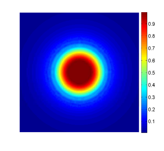
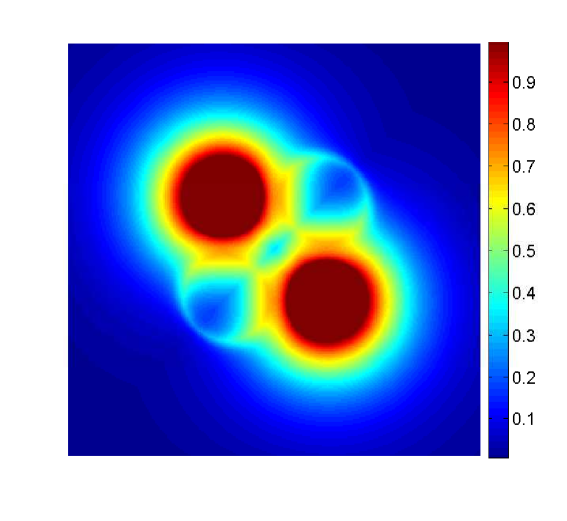
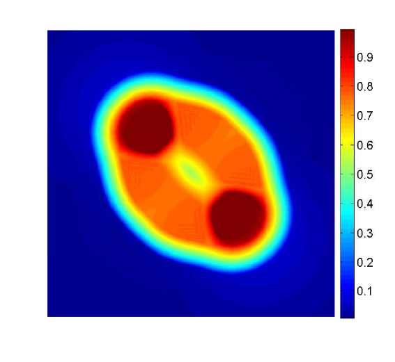
In this section, we provide two numerical examples to illustrate how the approximate solutions of the chemotaxis model (1.1) vary when changing the parameter from standard nonlinear diffusion () to doubly nonlinear diffusion (). For the discretization of both examples, a standard first order finite volume method (see the Appendix for details on the numerical scheme) on a regular mesh of 262144 control volumes is used. We choose a simple square domain and use the functions , and , along with parameters that are indicated separately for each case.
4.1. Example 1
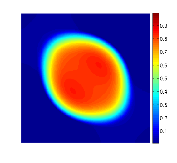
For the first example, we choose , , , and . The initial condition for the species density is given by
and the chemoattractant is assumed to have the uniform concentration . In a first simulation, we consider the simple case of and we compare the result with an analogous experiment with . We evolve the system until , and show in Figure 1 a snapshot of the cell density at this instant for both cases.
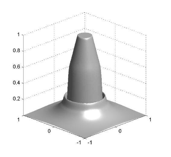
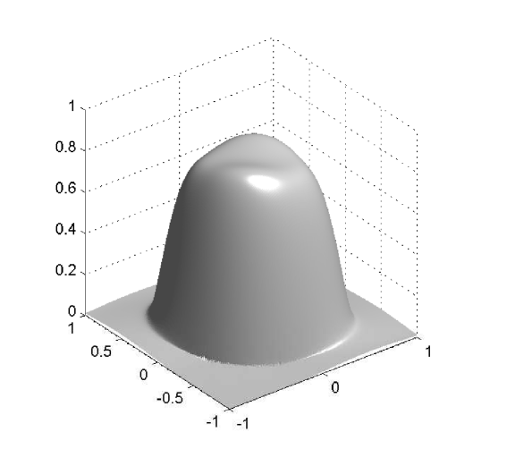
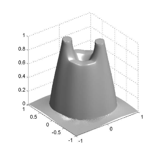
4.2. Example 2
 |
 |
 |
 |
 |
 |
 |
 |
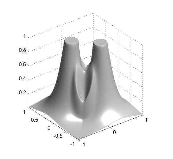
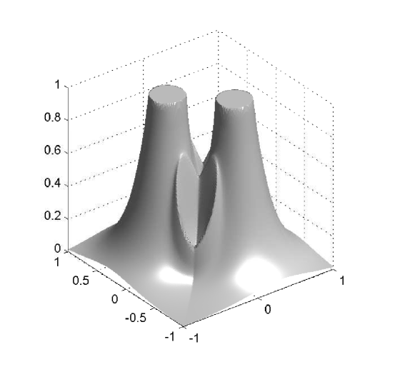
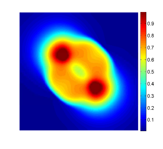
We now choose the parameters , , , and . The initial condition for the species density is given by
and for the chemoattractant
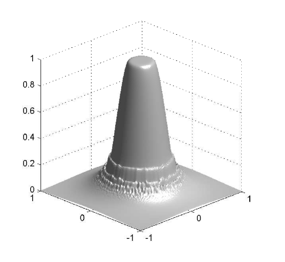
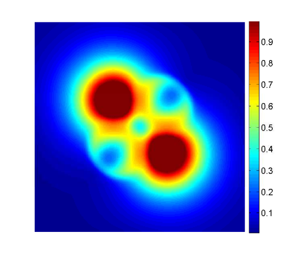
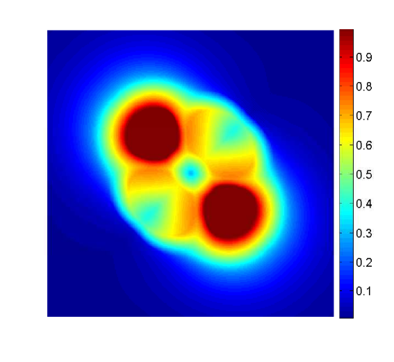
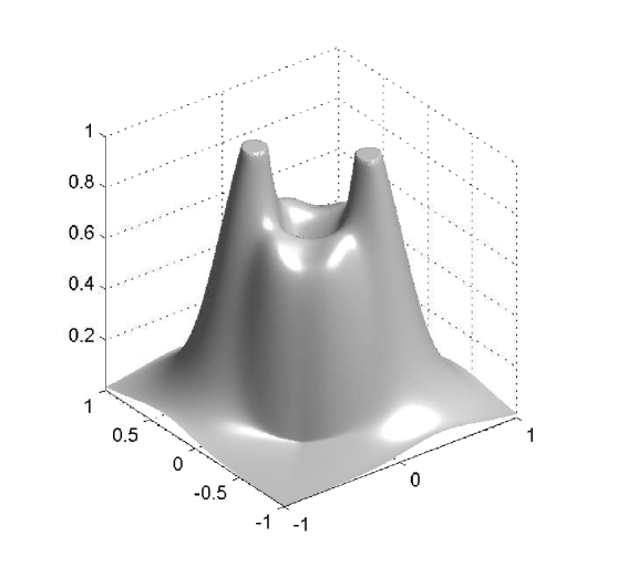
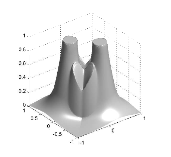
The behavior of the system for the cases and at different times is presented in Figures 2, 3 and 4.
 |
 |
 |
 |
4.3. Concluding remarks
W first mention that, from the previous examples, one observes that even though the numerical solutions obtained with differ from those obtained with , the qualitative structure of the solutions remains unchanged. We also stress that the numerical examples illustrate the effectiveness of the mechanism of prevention of overcrowding, or volume filling effect, since all solutions assume values between zero and one only. In particular, all examples exhibit plateau-like structures where , at least for small times, which diffuse very slowly, illustrating that the diffusion coefficient vanishes at (recall the special form of the functions and : they include the factor , and therefore the species diffusion and chemotactical cross diffusion terms vanish at and ).
In Example 2, the solution for has a smoother shape than the one for , which exhibits sharp edges. These sharp edges do not only appear for and , where one expects them, due to the degeneracy of the diffusion term and the choice of initial data, but also for intermediate solution values, as is illustrated by the plots for of Figures 2 and 3.
Acknowledgment
M. Bendahmane is supported by Fondecyt Project 1070682, and R. Bürger is supported by Fondecyt Project 1050728 and Fondap in Applied Mathematics (project 15000001). MB and RB also acknowledge support by CONICYT/INRIA project Bendahmane-Perthame. R. Ruiz acknowledges support by MECESUP project UCO0406 and CMUC. The research of J. Urbano was supported by CMUC/FCT and Project POCI/MAT/57546/2004. This work was developed during a visit of R. Ruiz to the Center for Mathematics at the University of Coimbra, Portugal.
Appendix
The definition of the finite volume method is based on the framework of [28]. An admissible mesh for is given by a family of control volumes of maximum diameter , a family of edges and a family of points . For , is the center of , is the set of edges of in the interior of , and the set of edges of on the boundary . For all , the transmissibility coefficient is
where denotes the common edge of neighboring finite volumes and . For and with common vertexes with , let ( for , respectively) be the open and convex polygon built by the convex envelope with vertices (, respectively) and . The domain can be decomposed into
For all , the approximation of is defined by
To discretize (1.1), we choose an admissible mesh of and a time step size . If is the smallest integer such that , then for .
We define cell averages of the unknowns , and over :
and the initial conditions are discretized by
We now give the finite volume scheme employed to advance the numerical solution from to , which is based on a simple explicit Euler time discretization. Assuming that at , the pairs are known for all , we compute from
Here denotes the discrete Euclidean norm. The Neumann boundary conditions are taken into account by imposing zero fluxes on the external edges.
References
- [1] Horstmann D. From 1970 until present: the Keller-Segel model in chemotaxis and its consequences, I. Jahresberichte der Deutschen Mathematiker-Vereinigung 2003; 105:103–165.
- [2] Keller EF, Segel LA. Model for chemotaxis. Journal of Theoretical Biology 1970; 30:225–234.
- [3] Murray JD. Mathematical Biology: II. Spatial Models and Biomedical Applications. Third Edition. Springer-Verlag: New York; 2003.
- [4] Bendahmane M, Karlsen KH, Urbano JM. On a two–sidedly degenerate chemotaxis model with volume–filling effect. Mathematical Models and Methods in Applied Sciences 2007; 17(5):783–804.
- [5] DiBenedetto E. Degenerate Parabolic Equations. Springer-Verlag: New York; 1993.
- [6] Urbano JM. The Method of Intrinsic Scaling. A Systematic Approach to Regularity for Degenerate and Singular PDEs. Lecture Notes in Mathematics, Vol. 1930. Springer-Verlag: New York; 2008.
- [7] Urbano JM. Hölder continuity of local weak solutions for parabolic equations exhibiting two degeneracies. Advances in Differential Equations 2001; 6:327–358.
- [8] Porzio M, Vespri V. Hölder estimates for local solutions of some doubly nonlinear degenerate parabolic equations. Journal of Differential Equations 1993; 103:146–178.
- [9] Gurney WSC, Nisbet RM. The regulation of inhomogeneous populations. Journal of Theoretical Biology 1975; 52:441–457.
- [10] Gurtin ME, McCamy RC. On the diffusion of biological populations. Mathematical Biosciences 1977; 33:35–49.
- [11] Witelski TP. Segregation and mixing in degenerate diffusion in population dynamics. Journal of Mathematical Biology 1997; 35:695–712.
- [12] Dkhil F. Singular limit of a degenerate chemotaxis-Fisher equation. Hiroshima Mathematical Journal 2004; 34:101–115.
- [13] Burger M, Di Francesco M, Dolak-Struss Y. The Keller-Segel model for chemotaxis with prevention of overcrowding: linear vs. nonlinear diffusion. SIAM Journal of Mathematical Analysis 2007; 38:1288–1315.
- [14] Herrero MA, Velázquez JJL. Chemotactic collapse for the Keller-Segel model. Journal of Mathematical Biology 1996; 35:177–194.
- [15] Yagi A. Norm behavior of solutions to a parabolic system of chemotaxis. Mathematica Japonica 1997; 45:241–265.
- [16] Amann H. Nonhomogeneous linear and quasilinear elliptic and parabolic boundary value problems. In: Function spaces, differential operators and nonlinear analysis, Teubner: Stuttgart; 1993: 9–126.
- [17] Laurençot P, Wrzosek D. A chemotaxis model with threshold density and degenerate diffusion. In: Chipot M, Escher J, Nonlinear Elliptic and Parabolic Problems: Progress in Nonlinear Differential Equations and their Applications. Birkhäuser: Boston; 2005: 273–290.
- [18] Drábek P. The -Laplacian—mascot of nonlinear analysis. Acta Mathematica Universitatis Comenianae 2007; 77:85–98.
- [19] Wu Z, Zhao J, Yin J, Li H. Nonlinear Diffusion Equations. World Scientific: Singapore; 2001.
- [20] Biler P, Wu G. Two-dimensional chemotaxis model with fractional diffusion. Mathematical Models in the Applied Sciences, in press.
- [21] Karlsen KH, Risebro NH. On the uniqueness and stability of entropy solutions of nonlinear degenerate parabolic equations with rough coefficients. Discrete and Continuous Dynamical Systems 2003; 9:1081–1104.
- [22] Ladyzhenskaya OA, Solonnikov V, Ural’ceva N. Linear and quasi-linear equations of parabolic type. American Mathematical Society: Providence; 1968.
- [23] DiBenedetto E, Urbano JM, Vespri V. Current issues on singular and degenerate evolution equations. In: Dafermos CM, Feireisl E (eds.), Handbook of Differential Equations, Evolutionary Equations, Vol. I. Elsevier/North-Holland: Amsterdam; 2004: 169–286.
- [24] Simon J. Compact sets in the space . Annali di Matematica Pura ed Applicata. Series IV 1987; 146:65–96.
- [25] Minty G. Monotone operators in Hilbert spaces. Duke Mathematics Journal 1962; 29:341–346.
- [26] Boccardo L, Murat F, Puel JP. Existence of bounded solutions for nonlinear elliptic unilateral problems. Annali di Matematica Pura ed Applicata. Series IV 1988; 152:183–196.
- [27] DiBenedetto E. On the local behaviour of solutions of degenerate parabolic equations with measurable coefficient. Annali della Scuola Normale Superiore di Pisa. Classe di Scienze. Serie IV 1986; 13:487–535.
- [28] Eymard T, Gallouët T, Herbin R. Finite volume methods. In: Ciarlet PG, Lions JL (eds.) Handbook of Numerical Analysis, vol. VII. North-Holland: Amsterdam; 2000: 713–1020.