On a Notion of Graph Centrality Based on Data Depth
Abstract
A new measure to assess the centrality of vertices in an undirected and connected graph is proposed. The proposed measure, centrality, can adequately handle graphs with weights assigned to vertices and edges. The study provides tools for graphical and multiscale analysis based on the centrality. Specifically, the suggested analysis tools include the target plot, centrality-based neighborhood, local centrality, multiscale edge representation, and heterogeneity plot and index. Most importantly, our work is closely associated with the concept of data depth for multivariate data, which allows for a wide range of practical applications of the proposed measure. Throughout the paper, we demonstrate our tools with two interesting examples: the Marvel Cinematic Universe movie network and the bill cosponsorship network of the 21st National Assembly of South Korea.
Keywords: Graph centrality; Data depth; Multiscale analysis; Visualization; Network data
1 Introduction
A fundamental and indispensable tool for analyzing graph data is a graph centrality measure, which evaluates the prominence of vertices in a given graph structure (Sabidussi, 1966; Freeman, 1978). Several measures have been suggested based on different concepts of what constitutes a ‘central’ vertex (see, e.g., Borgatti and Everett, 2006; Rodrigues, 2019). The concept of centrality has been developed primarily in social network analysis and, more broadly, in the field of social sciences (Wasserman and Faust, 1994).
Meanwhile, in statistics, the concept of data depth for multivariate data has been extensively studied since Tukey (1975). Data depth is a multivariate generalization of a univariate rank, but in a center-outward manner, starting from the deepest point(s) and extending towards the outer points. Notable instances of data depth include half-space depth (Tukey, 1975), simplical depth (Liu, 1990), projection depth (Zuo and Serfling, 2000a), and data depth (Vardi and Zhang, 2000), among others. See Zuo and Serfling (2000a); Mosler and Mozharovskyi (2022) for an extensive review. The data depth is a robust and nonparametric analytic tool for multivariate data. It is known for its powerful usage in robust estimation (Zuo et al., 2004), regression analysis (Rousseeuw and Hubert, 1999), and functional data analysis (López-Pintado and Romo, 2009; Sun and Genton, 2011).
Therefore, both graph centrality and data depth have a surprisingly comparable idea in that they measure the degree of ‘centralness’ of a point or a vertex w.r.t. a given set of data. Nevertheless, there are a limited number of studies that establish a connection between these two fields of research. Aamari et al. (2021) developed a data depth function by generating a neighborhood graph based on the provided multivariate data and calculating the centrality of that graph. Cerdeira and Silva (2021) introduced a new centrality measure, termed Tukey centrality, which leverages the popular concept of half-space depth. However, as indicated in the latter study, the computation of Tukey centrality is NP-hard, so there is no reason to prefer it over the existing ones. To our knowledge, these are the only works connecting the two fields.
The aim of this paper is to introduce a new centrality measure, called centrality, for vertices of an undirected and connected graph, analogous to the data depth of Vardi and Zhang (2000). This measure can handle graphs with weights assigned to both vertices and edges in a straightforward manner. Nevertheless, the computation of this measure is simple and does not entail a higher computational cost than the existing centrality measures, unlike the approach proposed by Cerdeira and Silva (2021). Furthermore, due to the connection between our work and the notion of data depth for multivariate data, there are several practical possibilities for expanding the proposed measure based on the extensive literature on data depth. For instance, the centrality-based neighborhood and the local centrality introduced in this study are closely related to the concept of local depth in Paindaveine and Van Bever (2013). In addition, we provide various graphical and multiscale analysis tools that rely on the centrality. The tools are based on an insightful interpretation of the suggested measure (Remark 1), distinguishing our centrality measure from others. Through these tools, we demonstrate that even the basic concept of centrality has a wide range of practical uses.
The rest of this paper is organized as follows. The centrality measure is defined in Section 2, and its properties are discussed, along with comparisons to the existing measures. Section 3 presents a visualization tool, the target plot, that utilizes the centrality. Section 4 expands upon the centrality measure using a multiscale approach. The centrality-based neighborhood of a vertex is precisely defined and utilized to derive the local centrality. The method for representing edges at multiple scales is also described. In Section 5, we propose a group heterogeneity index to analyze graph data effectively at the group level. In Sections 2–5, the Marvel Cinematic Universe movie network is utilized to aid our explanation. Then, in Section 6, we consider the bill cosponsorship network of 317 members in the 21st National Assembly of South Korea, which effectively demonstrates the practicality of the tools developed in the study. Finally, Section 7 provides concluding remarks with further discussion. All technical proofs are in the Appendix.
All methods and data sets used in this paper are provided via the R package L1centrality (Kang and Oh, 2024), available from the Comprehensive R Archive Network. Also, the codes for reproducing the figures and analysis in this paper are available from https://github.com/seungwoo-stat/L1centrality-paper.
2 Centrality Measure
2.1 Notations and Review of Graph Centrality Measures
Denote a graph by , where is a set of vertices (nodes, points, or actors), and is a set of edges (ties, or lines) connecting pairs of distinct vertices. The number of vertices, ( indicates the cardinality of the set), is often referred to as a graph size. When edges do not have direction, i.e., every connection from vertex to has a connection from to , we call the graph undirected. Otherwise, the graph is directed. Hereafter, we assume that the given graph is undirected.
The adjacency matrix is denoted by , where if and are directly connected by an edge and 0 otherwise. A sequence of edges connecting a set of vertices is called a path. A graph is said to be connected when it is possible to reach any vertex from any other vertex, that is, when a path always exists between any two vertices. Based on the paths, define , the geodesic distance between and , as the shortest path (geodesic path) length between and . Here, the path length is the sum of the weights of the edges of that path. When the edges of a graph all have weight 1, i.e., (edge) unweighted graph, the path length is simply equal to the number of edges in that path. Of course, this distance function satisfies all the properties of the usual distance function, such as triangle inequality and symmetry.
As noted, edges can have positive weights, which denote the distance between two nodes through the edge. Likewise, vertices can also have nonnegative weights, indicating the importance of that node. This could refer to the contextual information that reflects the significance of the vertices. For notational simplicity, we call vertex weights multiplicities and edge weights just weights since a weighted graph usually refers to a graph with edge weights, not vertex multiplicities.
The notion of centrality quantifies the ‘centralness’ of each vertex in a given graph structure. However, there is no consent to this concept, which has led to several definitions of centrality. We focus on three intuitive graph centrality measures listed below (Freeman, 1978). In the following definitions, we only consider connected and unweighted (all edge weights and all vertex multiplicities are set to 1) graphs.
-
1.
The degree centrality regards a vertex with many direct connections to other vertices as central. Specifically, degree centrality at vertex is defined as .
-
2.
The closeness centrality defines a vertex as central if it is close to all other vertices. In the formula, it is defined as the reciprocal of the sum of the distances to other nodes. That is, closeness centrality at vertex is .
-
3.
The betweenness centrality perceives that the vertex in the ‘middle’ of the geodesic paths has more influence. For , it is quantified as , where denotes the number of geodesic paths connecting and , and indicates the number of geodesic paths between and that pass through .
Other centrality measures include eigenvector centrality (Bonacich, 1972), hubs and authorities (Kleinberg, 1999), and much more variants. See e.g., Wasserman and Faust (1994, Chapter 5), Borgatti and Everett (2006), Rodrigues (2019) and references therein.
Each notion of graph centrality can possibly be generalized for graphs with weights and multiplicities. For example, denoting the multiplicity of vertex as , the degree centrality of can be generalized as . However, this generalization is forced, and there is no suitable explanation for why this should be the generalized form of the degree centrality, meaning that any variation similar to the above can be proposed. Likewise, the closeness centrality and betweenness centrality can be generalized in an arbitrary way. This is because these centrality measures were originally defined for unweighted graphs without consideration of handling weights. To our knowledge, there is no consensus on generalizing these centrality measures to (vertex and edge, but especially vertex) weighted graphs.
2.2 Motivation and Definition
Although there are many definitions of centrality, there is a similarity. It first defines a measure and then perceives the vertex with the highest measure as the most central node (hereafter, ‘center’). For example, for the betweenness centrality, one may ask, ‘What is the center vertex based on the betweenness centrality?’ One would answer, of course, ‘The vertex with the highest betweenness centrality.’
Our approach goes in the opposite direction from these traditional approaches. First, we define the notion of a center vertex. Next, we describe a centrality measure from this notion of center vertex. Roughly speaking, our approach quantifies how much a given node is related to the center vertex. This is the essential feature of the proposed measure, which we elaborate on after defining it.
Now, assume that a given graph has edge weights and vertex multiplicities. However, the graph is still assumed to be undirected and connected. For disconnected graphs, the proposed centrality measure can be applied to each connected component (maximal connected subgraph). The treatment of directed graphs will be discussed in Section 7. To this end, the notion of the center vertex, graph median, is defined below.
Definition 1 (Graph median (Hakimi, 1964)).
Given an undirected, connected graph with and multiplicity for each vertex, is called a graph median if it minimizes .
The definition of graph median can be seen as an analogous concept of a multivariate median or the median (Small, 1990; Vardi and Zhang, 2000). However, it is important to note that the median is unique unless multivariate points are collinear, i.e., all lie on a line (Small, 1990), whereas the graph median can have more than one element. For example, all vertices of a complete graph (without weights or multiplicities) are the graph median. Denote the set of graph medians of graph with multiplicities as . Based on the notion of graph median, the centrality measure is defined.
Definition 2 ( centrality measure).
Suppose that is an undirected, connected graph with and multiplicity for each vertex. Assuming that , the centrality of vertex is defined as
In other words, the centrality of a node is one minus the minimum amount of multiplicity that must be incremented for that node to become a graph median. This definition leads to the following closed-form formula for calculating the centrality measure,
| (2.1) |
where .
We make three notes. Firstly, the graph median always has an centrality of 1. Secondly, the centrality is always between 0 and 1 due to the triangle inequality applied to equation (2.1). Hence, a node with an centrality close to one indicates a central vertex. Moreover, since the measure is independent of the graph size , i.e., the measure is normalized, it is possible to compare the centrality values of vertices in different graphs. Notice that the above three centrality measures depend on the graph size and require suitable normalizations (Freeman, 1978). Lastly, when , the th term in the numerator of equation (2.1) is eliminated. In other words, assigning a multiplicity of zero to a particular vertex means disregarding its influence while calculating the centrality. Therefore, in most cases, all multiplicities are assigned a positive value unless one intends to disregard that vertex purposely.
Remark 1.
The essence of the proposed approach is that the centrality measure is defined based on the notion of graph median, which means that the proposed centrality ranks the relative importance of vertices w.r.t. the center vertex. Specifically, by incrementing the multiplicity of by , becomes the graph median. Hence, is the amount of multiplicity required to replace the original graph median by vertex . In other words, the greater the centrality, the higher the relevance of the vertex to the graph median. However, this is not the case with the above three centrality measures. For example, a vertex with a high betweenness centrality does not imply that the vertex is relevant to the vertex with the highest betweenness centrality. This concept is a useful and important aspect of the centrality, enabling further analysis tools in Sections 3 and 4.
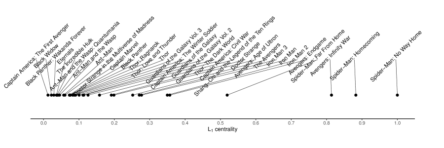
Example 1 ( centrality of the Marvel Cinematic Universe movies).
To facilitate the explanation of the proposed centrality measure, we proceed on a small toy network of Marvel Cinematic Universe (MCU) movies. This data set was first used by Choi and Oh (2021) to analyze graphs with signals. The data set consists of 32 movies from the MCU released between 2008 and 2023. Each movie represents one vertex in the graph. Since these movies share a common universe or plots, they often share casts. When there is at least one common cast between movies and , the edge is connected, with weight . Here is a set of cast from movie . In other words, if the proportion of common casts is large, the path length for that edge is small. We also used the worldwide gross of each movie (in USD, archived from IMDb (https://www.imdb.com) on Nov. 3rd, 2023) as the multiplicity of each vertex. Hence, the network is an undirected and connected graph with 32 vertices (with positive multiplicities) and 278 edges (with weights).
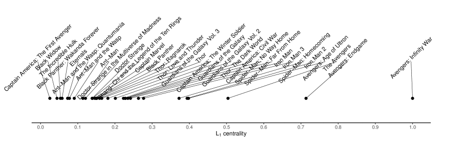
The centrality of each movie is shown in Figure 1. As expected, four Avengers series (Avengers: Infinity War (the graph median), Avengers: Endgame, The Avengers, Avengers: Age of Ultron), in which many heroes overlap with the other series, were the top four movies with the highest centrality. Furthermore, it is worth mentioning that these movies had high worldwide gross, highlighting their significant positions within the network. In other words, the context surrounding the box office performance of each movie is taken into account while calculating the centrality. The subsequent section mathematically addresses the influence of the multiplicity of a particular vertex on its centrality.
Before closing this section, we connect the proposed centrality to data depth literature. The definition of the centrality is analogous to the data depth of Vardi and Zhang (2000). However, the data depth is defined for any point (not necessarily a data point) in the sample space, while the centrality is only defined for vertices. Nevertheless, the notion of the centrality can be extended to an arbitrary point on existing edges. To simplify the definition, in Definition 1, we intentionally restricted the graph median to be found at the vertices. However, Hakimi (1964) called the graph median an absolute median and proposed a more generalized concept—it can be any point on the graph, not necessarily a vertex, and can be any point on an existing edge. Based on this definition, we may define centrality measure for an arbitrary point on the existing edges. In this paper, however, we only stick to vertex centrality. Graphs that an arbitrary point on the edge has an interpretable meaning are limited, and we leave this topic for future research.
2.3 Theoretical Properties
Theorem 1 (Properties of centrality).
Suppose that is an undirected, connected graph with , multiplicities for each vertex, and . The centrality measure has the following properties:
-
(P1)
Scale invariance: It is invariant to (positive) multiplicative transformations of vertex multiplicities and edge weights.
-
(P2)
Maximality: It is maximized to 1 if and only if the given vertex is the graph median. If , then . If , is the unique vertex with .
-
(P3)
Minumum value: .
-
(P4)
Minimum at infinity: Suppose that the subgraph induced by deleting vertex is connected. When is moved to infinity, that is, for all , and for all , then .
We assert that properties (P2) and (P3) align with our intuitive understanding of what constitutes a central vertex. The greater the multiplicity, the more likely the vertex is to have a large centrality. Throughout this paper, Theorem 1 will be used several times as we develop analysis tools based on the centrality.
In connecting the notion of graph centrality to the data depth studies, it is worth referring to the concept of statistical depth. In Zuo and Serfling (2000a), four properties of the data depth function were proposed, and a data depth function satisfying all these properties is called statistical depth. They are (i) affine invariance, (ii) maximality at the center, (iii) monotonicity relative to the deepest point, and (iv) vanishing at infinity. Property (P1) can be viewed as an analog of (i), and (P2) as (ii), and (P4) as (iv). However, we could not not find a property analogous to (iii).
2.4 Comparison and Computation
We compare the centrality measure to the three centrality measures outlined in Section 2.1. The centrality is most relevant to the closeness centrality of the three measures. If the closeness centrality is generalized as for , the centrality and the closeness centrality identify the same set of the center vertex (the graph median). Hence, the proposed measure and closeness centrality share a consensus on what the most central vertex is. However, they differ in the way they quantify and rank the centrality of vertices other than the graph median. We assert that the centrality is a more sophisticated measure than the closeness centrality. Recall equation (2.1),
In the numerator, we see that the reciprocals of the ’s closeness centrality appear. The larger the closeness centrality of , the larger is likely to be. However, what is also considered in the above equation is the closeness centrality of nearby vertices. Suppose that we have two vertices with the same closeness centrality. One is at the terminal, and the other is surrounded by many other vertices. A neighbor vertex connected by the former terminal vertex has a much higher closeness centrality because all geodesic paths from the terminal vertex must pass through the neighbor vertex; thus, the former terminal vertex is likely to have a small centrality.
In addition, as mentioned in Remark 1, the centrality is a natural ordering of vertices w.r.t. the graph median. This is what makes our measure different from the other three measures. It allows us to visualize the network based on the center, define a natural notion of the neighborhood that takes into account the whole graph structure, and localize the proposed centrality measure, enabling multiscale analysis.
Example 2 (Centrality measures applied to the MCU movie network).
We compare the degree, betweenness, and closeness centralities to the centrality measure. To this end, we used the MCU movie network with the same positive multiplicity for all vertices because the three centrality measures cannot be easily generalized for graphs with multiplicities. However, we kept edge weights since the closeness and betweenness centralities can incorporate edge weights while the degree centrality cannot.
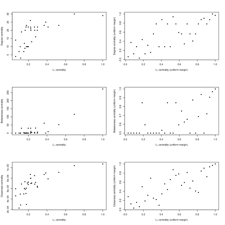
The Pearson correlation coefficients (Spearman rank correlation coefficients) of the centrality with the degree, betweenness, and closeness centrality measures were 0.6604 (0.7400), 0.8778 (0.6037), and 0.7317 (0.7852), respectively. Thus, the proposed centrality was positively correlated with the existing measures but was not equivalent to any of the three measures. That is, the rankings induced by the centrality measures are different. Another thing to note is that in the MCU movie network, the betweenness centrality treats half of the vertices as centrality zero, making comparing these vertices difficult. On the other hand, the centrality never treats any centrality as zero (Theorem 1 (P3)), and there are no ties between the centralities of 32 vertices. Scatter plots comparing the centrality with the three measures are provided in the Appendix B.
We next explain the practical computation procedure of the centrality. Suppose that the geodesic distance matrix is computed. Then, the computation of the centrality, , for all can be completed within computations (in big-O notation). Specifically, the vector of centralities, can be computed using the following formula,
| (2.2) |
where and . Moreover, division by a matrix is defined element-wise, and is applied to each element of the vector. The rowmax operation indicates the maximum element in each row, and when taking the rowmax operation, we ignore the diagonal terms or define .
Based on the above argument, the computational cost of the centrality is not greater than that of the closeness centrality and the betweenness centrality. This is because the bottleneck in computing the centrality is not in the computation of equation (2.2) but in the computation of the geodesic distance matrix . The computation of the geodesic matrix for an (edge) weighted graph can be achieved using the approach suggested by Dijkstra (1959) or the Floyd–Warshall algorithm (Floyd, 1962). The time complexity of these algorithms is . The time complexity can be reduced for sparse graphs using a special data structure (Fredman and Tarjan, 1984), but it is not lower than . Therefore, the computation of any centrality measure that needs to construct the geodesic distance (e.g., the closeness centrality and betweenness centrality) possesses a time complexity greater than or equal to the time complexity of the centrality computation.
3 Target Plot
In this section, we propose a novel graph visualization tool that aims to embed a graph onto a two-dimensional plane in a way that effectively represents the structural information of each vertex, specifically the centrality. As in the previous section, we examine a graph with vertices that is undirected, connected, and has weighted edges. However, we impose a constraint that all vertices have the same multiplicity, meaning that we exclusively examine vertex unweighted graphs. The reason for this restriction will be explained shortly.
Various graph drawing approaches are available for representing graphs on a two-dimensional plane, and each approach has a distinct perspective on what constitutes a visually pleasing representation. The algorithms proposed by Kamada and Kawai (1989) and Fruchterman and Reingold (1991) are often used in this domain. However, to our knowledge, none of the existing algorithms take graph centrality into account when deciding where to place points in their plot. Typical methods do not place the most central vertex in the center of the plot, nor do they put the least central vertex in the periphery.
In light of Remark 1, it is intuitive to position the graph median at the central point and the remaining vertices distributed around concentric circles whose radii correspond to their centrality. A graph is visually represented by the plot in a way that effectively conveys the structural characteristics of each vertex’s centrality. In pursuit of this objective, we present a method of plotting graphs called target plot.
-
1.
We aim to determine a configuration of points on a two-dimensional plane, with each vertex represented as an individual point. Let denote the point corresponding to vertex (). In circular coordinates, this point is denoted as . The target plot constraints to lie on a concentric circle with radii , so the graph median is placed at the center of the circles. The log transformation converts centralities in the interval to a radius in the interval . This transformation also reflects the observation that a vertex distant from all other vertices is likely to have a low centrality, according to equation (2.1) and Theorem 1 (P4). However, this observation may not be valid if there are distinct multiplicities on the vertices, i.e., a vertex far from all other vertices may exhibit high centrality if it has a high degree of multiplicity due to Theorem 1 (P3). For this reason, in this section, we focus only on unweighted vertex graphs.
-
2.
Next, we use the nonmetric multidimensional scaling method (nonmetric MDS; Kruskal, 1964a, b) with the constraint specified in 1. In essence, the goal is to find a configuration that retains the geodesic distances on the graph as much as possible while the constraint is enforced. Specifically, we aim to find a configuration of points that minimizes a metric called stress, adopted from Kruskal (1964a):
Here, , where denotes the usual Euclidean norm, and are chosen to minimize the stress metric given , subject to the following monotonicity condition:
There is a fast and efficient algorithm for fitting . See Kruskal (1964b) for details.
A starting configuration is set using the classical MDS (Mardia, 1978). If is the graph median, ; otherwise, is set to , where is the point representing as a result of classical MDS, and is the graph median with being the corresponding point derived from classical MDS. Given the configuration, it can be readily shown that
The gradient descent method is employed to iteratively update the value of until convergence. Specifically, denoting and , the gradient descent method is applied in a similar way to Kruskal (1964b): where (the relative magnitude of ), and is the step size with an initial value of 0.2 and is set to a smaller value by in each iteration. The above process is repeated until is small enough.
-
3.
From 1 and 2, we obtain a configuration representing the vertex . After plotting each point on a two-dimensional plane, contours of concentric circles are drawn to assist in recognizing and understanding the graph structure. For example, in Figure 2 (b), the radii of the four concentric circles correspond to the first (25%) to fourth (maximum) quartiles of the centralities. Hence, a quarter of the points lie within the smallest circle, and these points correspond to the vertices with the highest 25% centrality. From its appearance, it is clear why we call the resulting figure a target plot. This plot can be enhanced by including the color or shape of the points to facilitate more appropriate interpretation. For instance, there might be identifiable patterns in which the least central vertices share, indicating that it is desirable to remove vertices that exhibit those patterns before further analysis. This analysis will be demonstrated in Section 6.
Example 3 (Target plot of the MCU movie network).
Figure 2 shows two distinct methods of graph representation on a two-dimensional plane. Panel (a) displays the plot proposed by Fruchterman and Reingold (1991), and panel (b) shows the proposed target plot. Note that we used the same multiplicity for all vertices in this example. The target plot represents the structural information of centrality, showing the most central vertex (black point) and the least central vertex. In contrast, panel (a) does not convey this information.
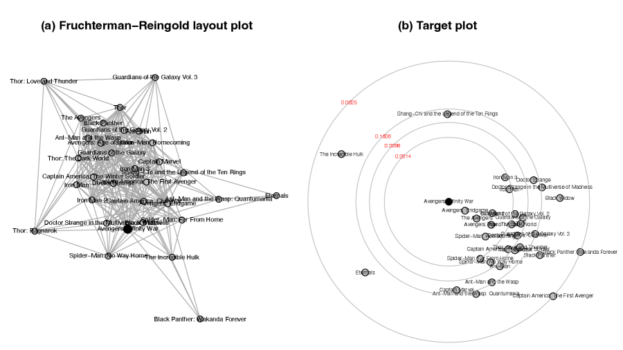
In the target plot, three points are far away from the rest: The Incredible Hulk, Shang-Chi and the Legend of the Ten Rings, and Eternals. These three movies are (the only) outliers in this distribution when computing the average geodesic distance of each movie to the others. In other words, the average distances of these three movies exceed the sum of 1.5 times the interquartile range and the third quartile of average distances. As a result, the target plot accurately represents the inherent structure of the network.
Before closing this section, we make three remarks. First, the concept of the target plot is not applicable to other graph centrality measures. A small problem is that the radii of each point cannot be determined using a straightforward log transformation. A crucial aspect is connected to Remark 1. For example, plotting vertices with high-degree centralities near the center of the concentric circles is utterly inadequate since it conveys the misleading impression that vertices with high-degree centralities are related. Second, the gradient descent method can converge to a local minimum of the stress measure, not an overall minimum. However, as Kruskal (1964b) pointed out, this is not a significant problem. The local minimum configuration is not the final result of the analysis, and it should be of interest if it is meaningful. Refer to the discussion in Kruskal (1964b, Section 5). Finally, the target plot resembles the depth contour, a visualization tool commonly used in data depth literature (e.g., Zuo and Serfling, 2000b). Depth contours, similar to our concentric circles, aid in identifying points with high and low data depths.
4 Local Centrality Measure
The degree centrality is a local measure considering only the vertices directly connected to a particular vertex. On the other hand, the closeness and betweenness centralities are global measures of centrality because they consider all vertices in the graph while calculating these measures. The centrality, in the same sense, is a global centrality measure. However, the structural properties of vertices can vary at both local and global scales, and all graph centrality measures, including the centrality, can only capture one of the two.
This section introduces a local extension of centrality based on the local depth proposed by Paindaveine and Van Bever (2013), where the degree of locality can be selected to a range of levels. This extension provides a multiscale view of a single graph with the centrality values at various locality levels. As described below, the local measure is derived by conditioning the graph to suitable centrality-based neighborhoods.
4.1 Centrality-Based Neighborhood
Referring back to Remark 1, vertices with high centrality can be considered neighborhoods of the graph median. This approach inherently considers the multiplicities of vertices and the geodesic distances when determining neighborhoods w.r.t. the graph median.
However, this approach is not applicable to vertices other than the graph median. To this end, we perform a symmetrization procedure analogous to Paindaveine and Van Bever (2013) that symmetrized a multivariate distribution for a specific point to derive depth-based neighborhoods of that point. Similarly, we symmetrize the graph w.r.t. a particular vertex, say , and set position to the graph median. The process is depicted in Figure 3, which shows a graph with seven vertices in the left panel. To create a symmetric graph for vertex C, we duplicate the entire graph, including the vertex multiplicities and edge weights, and overlap the original vertex C with the duplicated vertex C. Therefore, the multiplicity of vertex C is doubled, and the other copied vertices have the same multiplicity as the original, e.g., , where stands for the multiplicity of vertex A. This symmetrization procedure makes vertex C a graph median based on the following proposition.
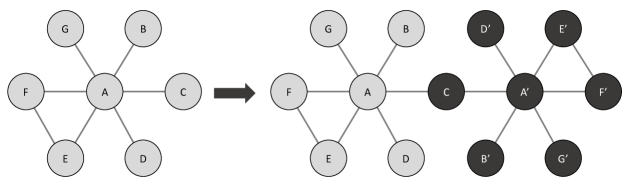
Proposition 1.
Suppose that is an undirected, connected graph with , a nonnegative multiplicity for vertex , , and . If is symmetrized w.r.t. vertex , then is a graph median. If , is the unique graph median in the symmetrized graph w.r.t. .
Therefore, the centralities of vertices in the symmetrized graph w.r.t. vertex will serve as a natural ordering of vertices in relation to . This results in the establishment of the centrality-based neighborhood.
Definition 3 ( centrality-based neighborhood).
The order centrality-based neighborhood of vertex is the set of vertices in the original graph, with centrality in the symmetrized graph w.r.t. larger than or equal to the % quantile of these centralities.
Of the vertices in the symmetrized graph, each copied vertex has the same centrality as the original vertex. Therefore, of the vertices in the original graph, about vertices are in the centrality-based neighborhood of each vertex. The parameter acts as a locality parameter, with smaller values corresponding to smaller neighborhoods. However, it would be demanding to construct a new geodesic matrix of size for the centrality computation each time a graph is symmetrized w.r.t. a specific vertex. Fortunately, it is unnecessary to compute a new distance matrix; this can be done by modifying only the multiplicities within the original graph.
Proposition 2.
Suppose that is an undirected, connected graph with and a nonnegative multiplicity for vertex , . If is symmetrized w.r.t. vertex , the centrality of vertex in the resulting graph is equal to the centrality of vertex in the original graph, but with the multiplicity of vertex substituted by , where .
For example, to calculate the centrality of vertex A in the right panel of Figure 3, it is enough to calculate the centrality of vertex A in the left panel, where the multiplicity of vertex C is substituted with (here, ). The geodesic distance matrix is calculated only once for the original graph and is subsequently utilized for computing centrality in the symmetrized graph.
Another significant implication of Proposition 2 is that the centrality-based neighborhood strikes a balance between vertices with high centrality (in the original graph) and vertices near the vertex of interest. Since the symmetrization w.r.t. vertex makes the graph median , vertices near are likely to have high centrality in the symmetrized graph. From another perspective, the centrality of the symmetrized graph is the same as the centrality of the original graph with multiplicities modified. Therefore, vertices with high centrality in the original graph are likely to have high centrality in the symmetrized graph.
Example 4 ( centrality-based neighborhood of Spider-Man: No Way Home).
By utilizing the MCU movie network and assigning vertex multiplicities based on the worldwide gross, we calculate the centrality of the graph symmetrized w.r.t. the vertex Spider-Man: No Way Home. The corresponding values are shown in Figure 4. The centrality-based neighborhood of the vertex Spider-Man: No Way Home is obtained using this ranking. For example, the order 5/32 centrality-based neighborhood refers to the five movies with the highest centralities in Figure 4. These vertices have large centralities in the original graph (Avengers series; see Figure 1) or are strongly linked to the vertex of interest (Spider-Man: Homecoming and Spider-Man: Far From Home are the two nearest (in geodesic distance) neighbors of Spider-Man: No Way Home in the MCU movie network).
Although the centrality-based neighborhood is developed to define the local centrality in the next section, it can also serve as a valuable tool on its own. For example, it can be used to recommend pertinent films to users who are interested in Spider-Man: No Way Home while simultaneously considering the significance (high centrality) in the entire network and relevance (small geodesic distance) to the target movie.
4.2 Local Centrality
Defining local centrality based on the above centrality-based neighborhood is straightforward: for each vertex, the graph is conditioned on the centrality-based neighborhood, and the local centrality is then computed from that graph. More precisely, we condition the graph in the sense defined below.
Definition 4 (Local centrality).
The order local centrality of vertex , denoted as , is the centrality of in the original graph, but only considering the centrality-based neighborhood of up to order during the computation. Specifically, denoting the set of order centrality-based neighborhood of as ,
| (4.1) |
In contrast to equation (2.1), the range of summation and maximum operations are confined to the centrality-based neighborhood. Therefore, calculating the local centrality by equation (4.1) is equivalent to computing the centrality of using equation (2.2), where the distance matrix and the multiplicity vector are replaced by a submatrix and a subvector of the original. The submatrix is formed by choosing the rows and columns corresponding to the indices of the order centrality-based neighborhood, and the subvector is a subset of the multiplicity vector corresponding to the order centrality-based neighborhood. Hence, the properties of the centrality, including Theorem 1, also apply to the local centrality. Clearly, the order 1 local centrality is identical to the centrality defined in Section 2. This measure will be referred to as global centrality.
Alternative to Definition 4, one might use the subgraph of the original graph, which is created by only considering the order centrality-based neighborhood of and edges that connect these vertices. However, we prefer Definition 4 for two reasons. First, when utilizing the subgraph, it is necessary to recalculate the distance matrix, which requires more computational effort, in contrast to the definition above, which only uses the submatrix of the original distance matrix. Second, especially for small values of , it cannot be ensured that the resulting subgraph is connected.
The definition of the local centrality is not to be confused with the centrality in the symmetrized graph defined in Section 4.1. The symmetrization procedure is used to identify the centrality-based neighborhood. Once the neighborhood is identified, the centrality values in the symmetrized graph are not used. The local centrality is computed in the original graph conditioned on these neighboring vertices.
Concerning Theorem 1 (P3), the local centrality is generally higher than the global centrality as the lower bound () increases. Therefore, rather than focusing on the absolute value of the local centrality, we propose to look at its relative value, i.e., its rank, compared to the local centrality of other vertices of the same order. Given these points, the local centrality provides a direct method to investigate the structure of a graph at different levels, depending on the value of . In Section 6, we show how to leverage the local centrality to perform a multiscale analysis of a graph.
4.3 Multiscale Edge Representation
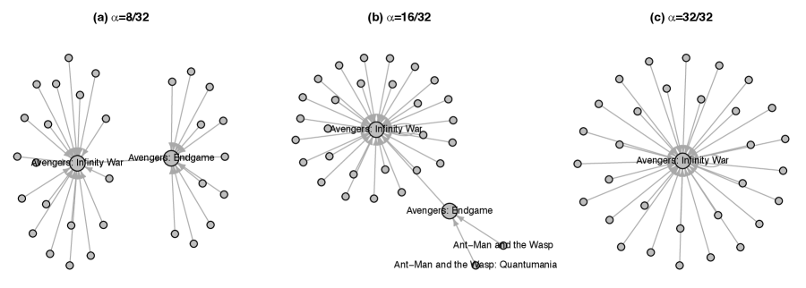
The local centrality defined in the previous section does not rank vertices based on the graph median. Instead, it quantifies the relevance of each vertex in relation to its local median, which is the graph median of the conditioned graph. Naturally, adopting the target plot in Section 3 for the local centralities with is not suitable since the concept of ranking w.r.t. the graph median no longer applies to local centralities. However, in this section, we present a multiscale visualization tool that uses the local centrality. The objective of this visualization method is to represent a given graph with approximately directed edges at different locality levels. The fundamental idea is similar to that of the target plot.
At a global level, the graph median can be regarded as the central point of the graph, as in the target plot. A given graph can be represented as a directed graph, where each vertex has an edge pointing to the graph median. At a locality level , we can construct a directed graph where each vertex is connected to its local median vertex determined at locality level . Edges are connected to each local median if more than one local median exists. Therefore, for every value of , the graph is represented as a directed graph containing about edges. The visualization of the directed graph also makes it easy to identify the local medians, facilitating further examination of that vertex.
Example 5 (Multiscale edge representation of the MCU movie network).
Figure 5 shows the directed graphs of the MCU movie network with multiplicities set to the worldwide gross. We selected three locality levels: , which means that we consider approximately 8, 16, and 32 vertices for each vertex when conditioning the graph and determining the centrality-based neighborhood and local median. In panel (a), it is evident that each vertex has either Avengers: Infinity War or Avengers: Endgame as a local median. The same applies to panel (b), where only two vertices from the Ant-Man and the Wasp series connect to Avengers: Endgame as a local median. Most vertices designate Avengers: Infinity War as the local median, which also serves as the graph median. Panel (c) provides a graph representation at the global level, where all vertices have edges directed toward the graph median. When comparing Figure 2 (a) to this multiscale edge representation, it is clear that the latter is significantly more comprehensible. The multiscale edge representation allows for a more precise visualization of the graph’s global and local structures, providing a multiscale perspective of a given graph.
5 Group Heterogeneity Index
This section provides a visualization tool and an index representing heterogeneity in the proposed centrality measures for groups of vertices or the entire graph. The proposed visualization tool and index are important for many types of analysis. For example, it can be used to evaluate if a group or graph exhibits any peculiar structural characteristics, detect trends across several groups or graphs (e.g., graphs that change over time), or explore the relationship of the heterogeneity of the group’s vertices to other attributes of the group. Furthermore, it can be employed to compare various groups and graphs and categorize them into similar types (Badham, 2013).
Several indices have been developed to quantify the heterogeneity of centrality measures. Some of the prominent measures in this field are the concept of centralization by Freeman (1978), the variance index of Snijders (1981), and the notion of hierarchization by Coleman (1964, Chapter 14). Recently, Badham (2013) discussed using the Gini coefficient to measure heterogeneity; the author argued that it has favorable theoretical characteristics compared to the previously discussed indices.
However, the Gini coefficient has yet to be well studied as a descriptive measure of centrality heterogeneity in network science. Interestingly, the Lorenz curve and Gini coefficient have been studied in data depth. Liu et al. (1999) used the Lorenz curve and Gini coefficient to establish a metric for quantifying kurtosis in multivariate data. Given that the notion of graph centrality in this study is based on a specific data depth, the purpose of this section is to revisit the Lorenz curve and Gini coefficient as a tool for analyzing the heterogeneity of the proposed global and local centrality measures. Here is a detailed description of the benefits of using these tools for global and local centralities.
The Lorenz curve is defined as follows. Given a univariate cumulative distribution function (cdf) with a nonnegative support, it is a plot of , with
| (5.1) |
where and (Gastwirth, 1971). By definition, is nondecreasing in and . Furthermore, and . Given centrality measurements, , of (5.1) is substituted by the empirical cdf , where denotes the indicator function. The Lorenz curve of the centrality measurements serves as an intuitive visual indicator of heterogeneity. The greater the deviation of the curve from the diagonal , the more it indicates that the group of vertices has a diverse structural attribute in a particular graph, i.e., their centralities show a high level of heterogeneity.
The Gini coefficient, defined as twice the area between the Lorenz curve and the diagonal , is a simple and widely used metric for quantifying the level of diversity in income and wealth, making it valuable for comparing multiple distributions. When is replaced with using the measurements , it can be readily verified that the Gini coefficient can be represented as
where . It is the expected difference of the centrality measurements with a suitable normalization. This also shows that the Gini coefficient is an appropriate index for quantifying heterogeneity among centrality values. Consistent with the results of the Lorenz curve, the larger the heterogeneity index, the less similar the nodes are in terms of centrality.
There are several advantages to using the Lorenz curve and Gini coefficient to quantify the heterogeneity of the proposed centrality. First, the Lorenz curve provides a visual diagnostic tool for comparing several groups or graphs rather than directly summarizing centrality values as a single number. Second, these tools are scale-invariant. As mentioned, local centralities generally exhibit higher values than global centralities. Consequently, the proposed method can be applied to compare heterogeneity across multiple locality levels, even if the scales of centralities across several locality levels differ. Third, the Gini coefficient is inherently standardized to 0 and 1. Some indices, such as centralization and variance, require a normalization procedure that normalizes the index w.r.t. the highest feasible value for a graph with the same number of vertices (Freeman, 1978; Snijders, 1981; Coleman, 1964). Moreover, these procedures only apply to graphs without weights, and it remains uncertain how similar normalization procedures may be implemented for the edge-weighted graphs considered in this study. Thus, the normalization procedure limits the applicability of given indices to the entire graph. In contrast, the Lorenz curve and Gini coefficient can be utilized for a set of vertices, not necessarily the entire graph, with the index inherently standardized.
Example 6 (Heterogeneity index of the MCU movie network).
We generate the Lorenz curve for the global centrality distribution of the MCU movie network using several multiplicities: (i) the same value, (ii) the worldwide gross, and (iii) the reciprocal of the worldwide gross. Figure 6 shows that the multiplicity of worldwide gross places the Lorenz curve below the curve with equivalent multiplicities (). This indicates that the centrality exhibits a higher level of heterogeneity, i.e., a larger Gini coefficient (), when measured with the worldwide gross as a multiplicity. That is, the centrality of the central nodes increases while the centrality of the outliers decreases. A simple regression analysis using worldwide gross as the independent variable and the centrality (with equal multiplicity) as the dependent variable confirms this view. The regression coefficient for the worldwide gross is statistically significant (-value ).
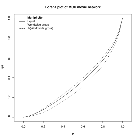
Alternatively, by defining the multiplicity as the inverse of the worldwide gross, we observe an upward shift of the Lorenz curve, indicating a decrease in the heterogeneity index (). This example shows that using the Lorenz curve and Gini coefficient as an index of heterogeneity is consistent with our understanding that assigning greater importance (multiplicity) to the central nodes amplifies the heterogeneity of the resulting centrality.
6 Application: South Korea’s National Assembly Bill Cosponsorship Network
In this section, we focus on the network of legislators in the 21st National Assembly of South Korea (May 30th, 2020–May 29th, 2024). Our main emphasis is on analyzing the network at multiple scales, demonstrating the utility of the tools presented so far. At the time of this writing, the 21st National Assembly is still in session, so our focus will be limited to the first 40 months of the assembly, from Jun. 2020 to Sep. 2023. In South Korea, a bill (legislative proposal) must be supported by at least 10 assembly members. We call them cosponsors of the bill. In this study, we do not distinguish between a member who presents the bill (as a representative) and those who cosponsor the bill. For simplicity, the term cosponsor is generically used in this section to refer to all members involved in the proposal. Therefore, the number of cosponsored bills by a member denotes the number of bills to which the person has agreed. Similarly, the number of cosponsored bills between two members indicates the number of bills the two members jointly supported.
A commonly used approach in the social sciences to identify assembly members’ social relationships is to build a network of them using bill cosponsorship information (Fowler, 2006)In this study, we constructed a graph of 317 assembly members, each representing a single vertex. An edge is established between two members if they have cosponsored at least one bill together. The weight of this edge is defined as the reciprocal of the number of cosponsored bills between two members, so the higher the number of cosponsored bills between two members, the shorter the path length between the corresponding vertices representing these members. A graph is formed by utilizing all 25164 bills proposed over 40 months, provided by the Bill Information System of the National Assembly of South Korea (https://likms.assembly.go.kr/bill/main.do). The resulting graph is undirected and connected, with 317 vertices and 47657 edges, each edge having a weight. The multiplicities of all vertices are set to 1. We refer to this network as the assembly network for the remainder of this paper.
As of Sep. 30th, 2023, the party composition of the 317 members is as follows (for simplicity, independent members are categorized by their former political party): There are two major parties, the Democratic Party with 184 members and the People Power Party with 123 members. Additionally, one minor party, the Justice Party, has six members. There are also four small parties with only one member each: the Basic Income Party, Hope of Korea, Progressive Party, and Transition Korea. Moreover, the 317 vertices comprise two groups: those who served as 21st National Assembly members for 40 months (281) and those who did not (36). The latter group includes members who started their term through a by-election, resigned, or lost their seat for any reason during the 40 months.
Figure 7 (a) is the target plot of the assembly network, which shows that the assembly network is organized into communities by the two major political parties. Furthermore, individuals absent from the office for 40 months exhibit lower global centrality, likely because their time in the assembly is shorter than that of the others, resulting in fewer opportunities to cosponsor bills and build relationships with other members. Therefore, we eliminate these vertices for further analysis, which can be seen as analogous to trimming in traditional statistical analysis. Furthermore, we have removed two chairpersons of the 21st National Assembly with inactive involvement in cosponsoring legislation. As a result, the assembly network is reduced to a subgraph of vertices and 38222 edges. This reduced network will be utilized for the remaining study.
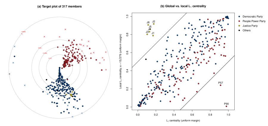
Next, we performed a multiscale analysis of the reduced assembly network. We calculated the global and local centrality for each member by setting the locality parameter to . Figure 7 (b) shows a graph comparing the global and local centrality values transformed to have a uniform margin. To facilitate explanation, we assign a random pseudonym to each member with a prefix indicating its political party. A notable observation is that vertices with high centralities also tend to have high local centralities. Similarly, vertices with low centralities also exhibit this phenomenon. Nevertheless, a small number of vertices do not follow this pattern. The six points in the top-left of the plot (J1–J6) and the two vertices in the bottom-right of the plot (P90 and P57) exhibit contrary behavior at the global and local levels. The paradoxical behavior of these eight vertices, which can be compared to the famous Simpson’s paradox, is worth examining.
-
•
All six members of the Justice Party (J1–J6) have low global centrality while demonstrating high local centrality at . This can be attributed to the fact that Justice Party members form a tight community with each other: the edges connecting Justice Party members are significantly stronger (i.e., lower edge weights) than those connecting a Justice Party member and a member from another party.
While examining the edges connected to one end of a particular Justice Party member, we consistently observed that the top five edges with the lowest weight were always connected to the other five Justice Party members. Table 1 also lists the number of cosponsored bills between the Justice Party members (i.e., the reciprocal of the edge weight connecting two Justice Party members). The magnitude of these values is relatively high for the entire population. The minimum number of cosponsored bills among the members of the Justice Party is 416 bills between J3 and J4, which falls in the 99.64% quantile in the distribution of the number of cosponsored bills among each member in the reduced assembly network. Hence, it is evident that the edge among the members of the Justice Party is solid.
Even so, the Justice Party members do not maintain a strong link with other party members. The highest number of cosponsored bills by each Justice Party member with a member of another party ranges between 221 and 317, much lower than the values in Table 1. This implies that the Justice Party is a cohesive community in which bill cosponsorship occurs primarily within the party. Therefore, inside the 15/279 centrality-based neighborhood of each Justice Party member, it is observed that there are four to six other Justice Party members included. As a result, each member of the Justice Party has a high level of centrality within the conditioned graph due to its cohesiveness.
Table 1: Number of cosponsored bills between each member of the Justice Party, and the total number of cosponsored bills by each member. J1 J2 J3 J4 J5 J6 J1 — 439 438 425 438 452 J2 439 — 421 418 416 417 J3 438 421 — 416 436 430 J4 425 418 416 — 431 427 J5 438 416 436 431 — 431 J6 452 417 430 427 431 — Total cosponsored bills 818 566 619 638 660 683 However, the total number of bills cosponsored by each member of the Justice Party is too small (last row of Table 1). The median number of cosponsored bills for all network members is 929, and the first quartile is 612. So, while these members are central within the party and their neighbors, the overall strength of those edges is not impressive. As a result, the global centrality is relatively low. This may be the behavior and strategy of a ‘niche’ party that is distinct from the legislative activity patterns of the major parties. They work together effectively, but their small party size limits their ability to engage actively in legislative action.
-
•
P57 and P90 exhibit contrasting behaviors to the members of the Justice Party. Their local centrality is low, but their global centrality is high, falling in the 91.40% (P57) and 97.85% (P90) quantiles of the global centrality distribution. This is because these two vertices essentially play an important role between the two major parties. As shown from the target plot in Figure 7 (a), each of the two major parties establishes a distinct community within the network. A few members, including P57 and P90, serve as a ‘bridge’ vertex between these two communities.
We started by counting cosponsored bills between and within both major political parties. The distribution is shown in Figure 8. There is a significant scarcity of bills cosponsored amongst members between the two parties compared to the bills cosponsored by the members of each party. That is, cosponsors of a bill typically consist of only Democratic Party members or only People Power Party members.
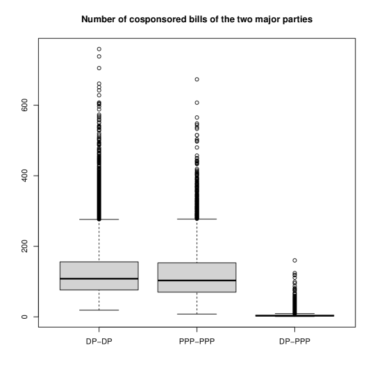
Figure 8: Distribution of the number of cosponsored bills within the Democratic Party (DP–DP), within the People Power Party (PPP–PPP), and between the two parties (DP–PPP). It is important to note that one network member has switched its affiliation from the Democratic Party to the People Power Party, hence being classified as a member of the People Power Party. This individual has cosponsored more bills with members of the Democratic Party than members of the People Power Party. So, except for this member, the top five highest number of cosponsored bills that occurred between the two major parties are as follows: P90–D139 (118 bills), P90–D63 (87 bills), P90–D128 (81 bills), P57–D140 (64 bills), and P8–D140 (60 bills). It is evident that P90 and P57 act as a ‘bridge’ between the two parties. Therefore, P90 and P57, along with vertices D139, D63, D128, D140, and P8, exhibit high global centrality. D128 is in the 72.40% quantile of the global centrality distribution, and the others are all above the 90% quantile.
However, among all the vertices with global centrality over the 90% quantile, P57 has the fewest cosponsored bills (467), and P90 has the second-fewest cosponsored bills (905). Furthermore, among the vertices with global centrality exceeding the 95% quantile, P90 has the fewest cosponsored bills, which means that the connection between each of the two vertices to its nearby vertices is weak (high edge weight). Therefore, rather than their closest neighbors, vertices with high global centrality are incorporated into the set of centrality-based neighbors for these vertices. This is a phenomenon contrary to that of the Justice Party members. Hence, a small centrality is obtained in the conditioned graph. In summary, the two exceptional vertices, P90 and P57, attain their high global centrality by serving as a ‘bridge’ between the two large communities in the network but have a weak connection to either of the communities.
The analysis presented demonstrates the utility of examining a single graph at multiple locality levels. Indeed, vertices with similar global centrality may exhibit contrasting behavior at a local level and vice versa. The proposed global and local centrality captures this specific aspect that cannot be accounted for by other centrality measures.
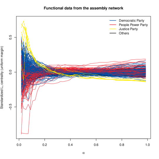
In this analysis, we used two values of and 1. However, a more refined multiscale analysis can be performed with densely chosen values of . By adjusting the locality level, we may create a functional data set in which each function corresponds to a member of the reduced assembly network. Figure 9 shows the variation in the local centrality of each vertex over . The local centrality values are transformed to a uniform margin for each locality level. For easier comprehension, each curve is then standardized to have a mean of zero, meaning that the average of the functional values is zero for each curve. The curves representing the Justice Party members deviate from the other curves. Collecting structural information of each vertex as a function can be more informative than other single-valued centrality measures. This functional data can be utilized for various analyses. For example, one can classify or cluster vertices or understand the relationship between the structural attribute of each vertex and other relevant characteristics. Extensive research on functional data analysis can be utilized with this data set (see, e.g., Ramsay and Silverman, 2005).
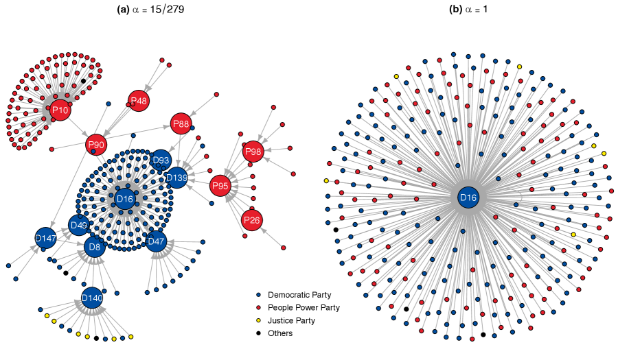
Finally, we present a multiscale edge representation of the reduced assembly network with two locality levels, and . In Figure 10, the local medians are represented by larger vertices, each labeled with the pseudonym of its member. Panel (a) reveals the presence of 15 local medians, with D16 being identified as the local median originating from nearly half of the vertices. As shown in panel (b), D16 serves as the graph median of the reduced assembly network. It would be worthwhile to investigate some local medians, such as D139, which serves as the local median for a number of People Power Party members, and D140, which is designated as the local median for all six Justice Party members. Altering the value of to different values makes a comprehensive multiscale representation of the assembly network possible. Conversely, a plot with all 38222 edges would be incomprehensible.
7 Discussion
In this paper, we have introduced the centrality for evaluating vertex centrality in graphs and related tools for multiscale and graphical analysis. The proposed method borrows ideas from existing literature on the data depth for multivariate data and particular instruments and methods used in the field. The tools provided in this paper are only a first step. There are many potential applications beyond the current discussion. The literature on data depth suggests various areas where the centrality can be used successfully. A few examples from the data depth literature include classification and clustering (Jörnsten, 2004; Li et al., 2012; Paindaveine and Van Bever, 2013), missing value imputation (Mozharovskyi et al., 2020), and nonparametric test (Liu and Singh, 1993).
This study only considered undirected graphs to define measures and tools. We briefly explore the potential extension of the concepts to directed graphs. In the literature, the concept of ‘centralness’ in directed graphs is divided into two distinct notions: prestige and centrality (Wasserman and Faust, 1994, Chapter 5.3). The prestige measure estimates the level of importance of a vertex in terms of receiving a choice. Conversely, the centrality measure in directed graphs assesses the level of importance in terms of giving a choice. It is feasible to extend the centrality to encompass directed graphs. Define the prestige for directed graphs in the following way. The graph median for prestige measure is redefined as the vertex that minimizes , where denotes the geodesic distance from to . Here, is not necessarily equal to , which means it is not a distance function. Assuming that every vertex can be reached from another, the prestige can be defined according to equation (2.1) with the indices in the function swapped. Nevertheless, since the triangle inequality, such as , does not necessarily hold—since is not a distance function—the resulting prestige measure cannot be ensured to fall within the range of . Together with the analogous theorem and propositions in this paper that apply to directed graphs, we plan to carry out a separate study on this topic elsewhere.
Next, recall that the concept of centrality is derived from the data depth. It is of interest to explore the theoretical connection between these two notions. A possible link can be made in the latent space model for graph data (Smith et al., 2019). In this model, edges are assumed to be generated depending on the positions of points in the underlying geometric space that represent the two vertices. With this model, we may ask if the centrality is a ‘good’ estimate of the depth w.r.t. the underlying probability distribution in the latent space. Then, we can consider the centrality as a desirable statistic rather than an ad-hoc measure. This can also construct a comprehensive distribution theory for a centrality statistic. For example, the large sample () behaviors of the centralities. We have established a proposition that may be useful for further study.
Proposition 3.
Let be a convex -dimensional space. Given , suppose that are i.i.d. samples from some probability distribution supported on , which we assume to have a density , bounded away from zero: for all . Multiplicities of are respectively, and . Then, the following strong consistency to the depth of w.r.t. , denoted as , holds. That is, with the usual Euclidean norm ,
The LHS is similar to equation (2.1), except that instead of using geodesic distance in the graph, it uses the Euclidean norm. Thus, if the geodesic distance in the graph approaches the Euclidean distance in the underlying geometric space at a suitable speed, it is possible to establish the convergence of the centrality to the depth in the latent space. Much literature proves that the geodesic distance in the graph converges to the geodesic distance in various latent space models (Alamgir and von Luxburg, 2012; Hwang et al., 2016). Nevertheless, there is uncertainty about which latent space models may effectively achieve the desired convergence speed and the conditions necessary to establish a concrete connection between the two concepts. This topic can be explored in future research, perhaps with a graph centrality based on the notion of another data depth function.
Acknowledgements
This research was supported by the National Research Foundation of Korea (NRF) funded by the Korea government (2021R1A2C1091357).
Data Availability
The MCU movie network and the assembly network are available from the R package L1centrality (https://CRAN.R-project.org/package=L1centrality).
References
- Aamari et al. (2021) E. Aamari, E. Arias-Castro, and C. Berenfeld. From graph centrality to data depth. arXiv preprint arXiv:2105.03122, 2021.
- Alamgir and von Luxburg (2012) M. Alamgir and U. von Luxburg. Shortest path distance in random -nearest neighbor graphs. In Proceedings of the 29th International Conference on Machine Learning, pages 1251–1258, 2012.
- Badham (2013) J. M. Badham. Commentary: Measuring the shape of degree distributions. Network Science, 1(2):213–225, 2013.
- Bonacich (1972) P. Bonacich. Factoring and weighting approaches to status scores and clique identification. Journal of Mathematical Sociology, 2(1):113–120, 1972.
- Borgatti and Everett (2006) S. P. Borgatti and M. G. Everett. A graph-theoretic perspective on centrality. Social Networks, 28(4):466–484, 2006.
- Cerdeira and Silva (2021) J. O. Cerdeira and P. C. Silva. A centrality notion for graphs based on Tukey depth. Applied Mathematics and Computation, 409:126409, 2021.
- Choi and Oh (2021) G. Choi and H.-S. Oh. Heavy-snow transform: A new method for graph signals. Unpublished Manuscript, 2021.
- Coleman (1964) J. S. Coleman. Introduction to Mathematical Sociology. Free Press, New York, 1964.
- Dijkstra (1959) E. W. Dijkstra. A note on two problems in connexion with graphs. Numerische Mathematik, 1:269–271, 1959.
- Floyd (1962) R. W. Floyd. Algorithm 97: shortest path. Communications of the ACM, 5(6):345, 1962.
- Fowler (2006) J. H. Fowler. Connecting the congress: A study of cosponsorship networks. Political Analysis, 14(4):456–487, 2006.
- Fredman and Tarjan (1984) M. Fredman and R. Tarjan. Fibonacci heaps and their uses in improved network optimization algorithms. In 25th Annual Symposium on Foundations of Computer Science, pages 338–346, 1984.
- Freeman (1978) L. C. Freeman. Centrality in social networks: Conceptual clarification. Social Networks, 1(3):215–239, 1978.
- Fruchterman and Reingold (1991) T. M. Fruchterman and E. M. Reingold. Graph drawing by force-directed placement. Software: Practice and Experience, 21(11):1129–1164, 1991.
- Gastwirth (1971) J. L. Gastwirth. A general definition of the Lorenz curve. Econometrica, 39(6):1037–1039, 1971.
- Hakimi (1964) S. L. Hakimi. Optimum locations of switching centers and the absolute centers and medians of a graph. Operations Research, 12(3):450–459, 1964.
- Hwang et al. (2016) S. J. Hwang, S. B. Damelin, and A. O. Hero, III. Shortest path through random points. The Annals of Applied Probability, 26(5):2791–2823, 2016.
- Jörnsten (2004) R. Jörnsten. Clustering and classification based on the data depth. Journal of Multivariate Analysis, 90(1):67–89, 2004.
- Kamada and Kawai (1989) T. Kamada and S. Kawai. An algorithm for drawing general undirected graphs. Information Processing Letters, 31(1):7–15, 1989.
- Kang and Oh (2024) S. Kang and H.-S. Oh. L1centrality: Graph/Network Analysis Based on L1 Centrality, 2024. URL https://CRAN.R-project.org/package=L1centrality. R package version 0.0.3.
- Kleinberg (1999) J. M. Kleinberg. Authoritative sources in a hyperlinked environment. Journal of the ACM, 46(5):604–632, 1999.
- Kruskal (1964a) J. B. Kruskal. Multidimensional scaling by optimizing goodness of fit to a nonmetric hypothesis. Psychometrika, 29(1):1–27, 1964a.
- Kruskal (1964b) J. B. Kruskal. Nonmetric multidimensional scaling: A numerical method. Psychometrika, 29(2):115–129, 1964b.
- Li et al. (2012) J. Li, J. A. Cuesta-Albertos, and R. Y. Liu. DD-classifier: Nonparametric classification procedure based on DD-plot. Journal of the American Statistical Association, 107(498):737–753, 2012.
- Liu (1990) R. Y. Liu. On a notion of data depth based on random simplices. The Annals of Statistics, 18(1):405–414, 1990.
- Liu and Singh (1993) R. Y. Liu and K. Singh. A quality index based on data depth and multivariate rank tests. Journal of the American Statistical Association, 88(421):252–260, 1993.
- Liu et al. (1999) R. Y. Liu, J. M. Parelius, and K. Singh. Multivariate analysis by data depth: descriptive statistics, graphics and inference, (with discussion and a rejoinder by Liu and Singh). The Annals of Statistics, 27(3):783–858, 1999.
- López-Pintado and Romo (2009) S. López-Pintado and J. Romo. On the concept of depth for functional data. Journal of the American Statistical Association, 104(486):718–734, 2009.
- Mardia (1978) K. V. Mardia. Some properties of clasical multi-dimesional scaling. Communications in Statistics-Theory and Methods, 7(13):1233–1241, 1978.
- Mosler and Mozharovskyi (2022) K. Mosler and P. Mozharovskyi. Choosing among notions of multivariate depth statistics. Statistical Science, 37(3):348–368, 2022.
- Mozharovskyi et al. (2020) P. Mozharovskyi, J. Josse, and F. Husson. Nonparametric imputation by data depth. Journal of the American Statistical Association, 115(529):241–253, 2020.
- Paindaveine and Van Bever (2013) D. Paindaveine and G. Van Bever. From depth to local depth: A focus on centrality. Journal of the American Statistical Association, 108(503):1105–1119, 2013.
- Ramsay and Silverman (2005) J. O. Ramsay and B. W. Silverman. Functional Data Analysis. Springer, New York, NY, USA, second edition, 2005.
- Rodrigues (2019) F. A. Rodrigues. Network centrality: An introduction. In E. E. N. Macau, editor, A Mathematical Modeling Approach from Nonlinear Dynamics to Complex Systems, pages 177–196, Cham, Springer, 2019.
- Rousseeuw and Hubert (1999) P. J. Rousseeuw and M. Hubert. Regression depth. Journal of the American Statistical Association, 94(446):388–402, 1999.
- Sabidussi (1966) G. Sabidussi. The centrality index of a graph. Psychometrika, 31(4):581–603, 1966.
- Small (1990) C. G. Small. A survey of multidimensional medians. International Statistical Review, 58(3):263–277, 1990.
- Smith et al. (2019) A. L. Smith, D. M. Asta, and C. A. Calder. The geometry of continuous latent space models for network data. Statistical Science, 34(3):428, 2019.
- Snijders (1981) T. A. Snijders. The degree variance: An index of graph heterogeneity. Social Networks, 3(3):163–174, 1981.
- Sun and Genton (2011) Y. Sun and M. G. Genton. Functional boxplots. Journal of Computational and Graphical Statistics, 20(2):316–334, 2011.
- Tian et al. (2002) X. Tian, Y. Vardi, and C.-H. Zhang. -depth, depth relative to a model, and robust regression. In Y. Dodge, editor, Statistical Data Analysis Based on the -Norm and Related Methods, pages 285–299, Basel, Birkhäuser, 2002.
- Tukey (1975) J. W. Tukey. Mathematics and the picturing of data. In Proceedings of the International Congress of Mathematicians, volume 2, pages 523–531, Vancouver, 1975.
- Vardi and Zhang (2000) Y. Vardi and C.-H. Zhang. The multivariate -median and associated data depth. Proceedings of the National Academy of Sciences, 97(4):1423–1426, 2000.
- Wasserman and Faust (1994) S. Wasserman and K. Faust. Social Network Analysis: Methods and Applications. Structural Analysis in the Social Sciences. Cambridge University Press, Cambridge, 1994.
- Zuo and Serfling (2000a) Y. Zuo and R. Serfling. General notions of statistical depth function. The Annals of Statistics, 28(2):461–482, 2000a.
- Zuo and Serfling (2000b) Y. Zuo and R. Serfling. Structural properties and convergence results for contours of sample statistical depth functions. The Annals of Statistics, 28(2):483–499, 2000b.
- Zuo et al. (2004) Y. Zuo, H. Cui, and X. He. On the Stahel–Donoho estimator and depth-weighted means of multivariate data. The Annals of Statistics, 32(1):167–188, 2004.
Appendix
Appendix A Proofs
A.1 Proof of Theorem 1
Proof.
-
(P1)
This is immediate from equation (2.1).
-
(P2)
It suffices to show that is the graph median if and the unique graph median if . Observe that for , by the triangle inequality. This yields that if . In addition, if .
-
(P3)
Suppose that is not a graph median. Due to (P2), becomes the graph median when multiplicity is incremented by . This is because the multiplicity of is after incrementing, and the sum of all vertices’ multiplicities is . Hence, . If is the graph median, . Thus, .
-
(P4)
Since the subgraph induced by deleting vertex is connected, it means that converges to a finite value for any , as is moved to infinity. Observe that
Hence, . ∎
A.2 Proof of Proposition 1
A.3 Proof of Proposition 2
Proof.
Without loss of generality, suppose that is symmetrized w.r.t. vertex . Denote the copied vertices with ‘prime’ on their index, e.g., is the copy of . In the symmetrized graph, the centrality of vertex is
Here, the numerator is given as
where
Hence, the centrality of vertex in the symmetrized graph is equivalent to the centrality of in the original graph with multiplicities . ∎
A.4 Proof of Proposition 3
Proof.
Let and . According to Vardi and Zhang (2000) and Tian et al. (2002), , and a.s. as by the strong law of large numbers (SLLN).
If , Vardi and Zhang (2000) proved that is the median w.r.t. . Hence, by the SLLN, the numerator of the LHS in the proposition converges to a nonpositive number a.s., which means that the LHS converges to a.s. In the rest of the proof, we assume .
Set and let be the closest random point to among . Here, and , as (e.g., take ). Then, for a sufficiently large ,
for some constant that depends on . Elaborating, due to the convexity of , a ball with center and radius will be inside , for a sufficiently large . The first inequality is derived from the probability that all to be located outside this ball, and the second inequality is immediate from , which holds for all .
Since as , Borel–Cantelli lemma can be applied to say that a.s. as . This further implies that
and thus, with probability one,
where as .
Using these facts, we get that, with probability one,
| (A.1) |
By the dominated convergence theorem, the RHS of equation (A.1) converges to the following value a.s.
where the first equality is derived by differentiation.
Appendix B Comparing Centrality Measure to Other Measures
The first column of Figure 11 shows the centrality versus the three centralities. The second column transforms computed centralities to a uniform margin for easy comparison, i.e., the lowest centrality is converted to , the second lowest to , and so on. Thus, if the rankings from the centrality measures are the same, every point would fall on the diagonal line, which is not valid for all plots in the second column.