On a Security vs Privacy Trade-off in Interconnected Dynamical Systems

Vaibhav Katewa¹, Rajasekhar Anguluri², Fabio Pasqualetti² ¹Department of Electrical Communication Engineering, Indian Institute of Science, Bangalore ²Department of Mechanical Engineering, University of California, Riverside, CA, USA

Abstract

We study a security problem for interconnected systems, where each subsystem aims to detect local attacks using local measurements and information exchanged with neighboring subsystems. The subsystems also wish to maintain the privacy of their states and, therefore, use privacy mechanisms that share limited or noisy information with other subsystems. We quantify the privacy level based on the estimation error of a subsystem’s state and propose a novel framework to compare different mechanisms based on their privacy guarantees. We develop a local attack detection scheme without assuming the knowledge of the global dynamics, which uses local and shared information to detect attacks with provable guarantees. Additionally, we quantify a trade-off between security and privacy of the local subsystems. Interestingly, we show that, for some instances of the attack, the subsystems can achieve a better detection performance by being more private. We provide an explanation for this counter-intuitive behavior and illustrate our results through numerical examples.

keywords:

Privacy , Attack-detection , Interconnected Systems , Chi-squared test

^t1^t1footnotetext: This material is based upon work supported in part by ARO award 71603NSYIP and in part by UCOP award LFR-18-548175.^t2^t2footnotetext: Email addresses: vkatewa@iisc.ac.in (Vaibhav Katewa), {rangu003, fabiopas}@engr.ucr.edu (Rajasekhar Anguluri, Fabio Pasqualetti)

1 Introduction

Dynamical systems are becoming increasingly more distributed, diverse, complex, and integrated with cyber components. Usually, these systems are composed of multiple subsystems, which are interconnected among each other via physical, cyber and other types of couplings [1]. An example of such system is the smart city, which consists of subsystems such as the power grid, the transportation network, the water distribution network, and others. Although these subsystems are interconnected, it is usually difficult to directly measure the couplings and dependencies between them [1]. As a result, they are often operated independently without the knowledge of the other subsystems’ models and dynamics.

Modern dynamical systems are also increasingly more vulnerable to cyber/physical attacks that can degrade their performance or may even render them inoperable [2]. There have been many recent studies on analyzing the effect of different types of attacks on dynamical systems and possible remedial strategies (see [3] and the references therein). A key component of these strategies is detection of attacks using the measurements generated by the system. Due to the autonomous nature of the subsystems, each subsystem is primarily concerned with detection of local attacks which affect its operation directly. However, local attack detection capability of each subsystem is limited due to the absence of knowledge of the dynamics and couplings with external subsystems. One way to mutually improve the detection performance is to share information and measurements among the subsystems. However, these measurements may contain some confidential information about the subsystem and, typically, subsystem operators may be willing to share only limited information due to privacy concerns. In this paper, we propose a privacy mechanism that limits the shared information and characterize its privacy guarantees. Further, we develop a local attack detection strategy using the local measurements and the limited shared measurements from other subsystems. We also characterize the trade-off between the detection performance and the amount/quality of shared measurements, which reveals a counter-intuitive behavior of the involved chi-squared $(\chi^{2})$ detection scheme.

Related Work: Centralized attack detection and estimation schemes in dynamical systems have been studied in both deterministic [4, 5, 6] and stochastic [7, 8] settings. Recently, there has also been studies on distributed attack detection including information exchange among the components of a dynamical system. Distributed strategies for attacks in power systems are presented in [9, 10, 11]. In [5, 12], centralized and decentralized monitor design was presented for deterministic attack detection and identification. In [13, 14], distributed strategies for joint attacks detection and state estimation are presented. Residual based tests [15] and unknown-input observer-based approaches [16] have also been proposed for attack detection. A comparison between centralized and decentralized attack detection schemes was presented in [17].The local detectors in [17] use only local measurements, whereas we allow the local detectors to use measurements from other subsystems as well.

Distributed fault detection techniques requiring information sharing among the subsystems have also been widely studied. In [18, 19, 20, 21, 22], fault detection for non-linear interconnected systems is presented. These works typically use observers to estimate the state/output, compute the residuals and compare them with appropriate thresholds to detect faults. For linear systems, distributed fault detection is studied using consensus-based techniques in [23, 24] and unknown-input observer-based techniques in [25].

There have also been recent studies related to privacy in dynamical systems. Differential privacy based mechanisms in the context of consensus, filtering and distributed optimization have been proposed (see [26] and the references therein). These works develop additive noise-based privacy mechanisms, and characterize the trade-offs between the privacy level and the control performance. Other privacy measures based on information theoretic metrics like conditional entropy [27], mutual information [28, 29] and Fisher information [30] have also been proposed. In [31], a privacy vs. cooperation trade-off for multi-agent systems was presented. In [32], a privacy mechanism for consensus was presented, where privacy is measured in terms of estimation error covariance of the initial state. The authors in [33] showed that the privacy mechanism can be used by an attacker to execute stealthy attacks in a centralized setting.

In contrast to these works, we identify a novel and counter-intuitive trade-off between security and privacy in interconnected dynamical systems. In a preliminary version of this work [34], we compared the detection performance between the cases when the subsystems share full measurements (no privacy mechanism) and when they do not share any measurements. In this paper, we introduce a privacy framework and present an analytic characterization of privacy-performance trade-offs.

Contributions: The main contributions of this paper are as follows. First, we propose a privacy mechanism to keep the states of a subsystem private from other subsystems in an interconnected system. The mechanism limits both the amount and quality of shared measurements by projecting them onto an appropriate subspace and adding suitable noise to the measurements. This is in contrast to prior works which use only additive noise for privacy. We define a privacy ordering and use it to quantify and compare the privacy of different mechanisms. Second, we propose and characterize the performance of a chi-squared ( $\chi^{2}$ ) attack detection scheme to detect local attacks in absence of the knowledge of the global system model. The detection scheme uses local and received measurements from neighboring subsystems. Third, we characterize the trade-off between the privacy level and the local detection performance in both qualitative and quantitative ways. Interestingly, our analysis shows that in some cases both privacy and detection performance can be improved by sharing less information. This reveals a counter-intuitive behavior of the widely used $\chi^{2}$ test for attack detection [7, 8, 35], which we illustrate and explain.

Mathematical notation: $\text{Tr}(\cdot)$ , $\text{Im}(\cdot)$ , $\text{Null}(\cdot)$ and
$\text{Rank}(\cdot)$ denote the trace, image, null space, and rank of a matrix, respectively. $(\cdot)^{\mathsf{T}}$ and $(\cdot)^{+}$ denote the transpose and Moore-Penrose pseudo-inverse of a matrix. A positive (semi)definite matrix $A$ is denoted by $A>0$ $(A\geq 0)$ . $\text{diag}(A_{1},A_{2},\cdots,A_{n})$ denotes a block diagonal matrix whose block diagonal elements are $A_{1},A_{2},\cdots,A_{n}$ . The identity matrix is denoted by $I$ (or $I_{n}$ to denote its dimension explicitly). A scalar $\lambda\in\mathbb{C}$ is called a generalized eigenvalue of $(A,B)$ if $(A-\lambda B)$ is singular. $\otimes$ denotes the Kronecker product. A zero mean Gaussian random variable $y$ is denoted by $y\sim\mathcal{N}(0,\Sigma_{y})$ , where $\Sigma_{y}$ denotes the covariance of $y$ . The (central) chi-square distribution with $q$ degrees of freedom is denoted by $\chi_{q}^{2}$ and the noncentral chi-square distribution with noncentrality parameter $\lambda$ is denoted by $\chi_{q}^{2}(\lambda)$ . For $x\geq 0$ , let $\mathcal{Q}_{q}(x)$ and $\mathcal{Q}_{q}(x;\lambda)$ denote the right tail probabilities of a chi-square and noncentral chi-square distributions, respectively.

2 Problem Formulation

We consider an interconnected discrete-time LTI dynamical system composed of $N$ subsystems. Let $\mathcal{S}\triangleq\{1,2,\cdots,N\}$ denote the set of all subsystems and let $\mathcal{S}_{-i}\triangleq\mathcal{S}\setminus\{i\}$ , where $\setminus$ denotes the exclusion operator. The dynamics of the subsystems are given by:

	$\displaystyle x_{i}(k+1)$	$\displaystyle=A_{i}x_{i}(k)+{B_{i}}x_{-i}(k)+w_{i}(k),$		(1)
	$\displaystyle y_{i}(k)$	$\displaystyle=C_{i}x_{i}(k)+v_{i}(k)\qquad\quad i\in\mathcal{S},$		(2)

where $x_{i}\in\mathbb{R}^{n_{i}}$ and $y_{i}\in\mathbb{R}^{p_{i}}$ are the state and output/measurements of subsystem $i$ , respectively. Let $n\triangleq\sum_{i=1}^{N}n_{i}$ . Subsystem $i$ is coupled with other subsystems through the interconnection term ${B_{i}}x_{-i}(k)$ , where $x_{-i}\triangleq[x_{1}^{\mathsf{T}},\cdots,x_{i-1}^{\mathsf{T}},x_{i+1}^{\mathsf{T}},\cdots,x_{N}^{\mathsf{T}}]^{\mathsf{T}}\in\mathbb{R}^{n-n_{i}}$ denotes the states of all other subsystems. We refer to $x_{-i}$ as the interconnection signal. Further, $w_{i}\in\mathbb{R}^{n_{i}}$ and $v_{i}\in\mathbb{R}^{p_{i}}$ are the process and measurement noise, respectively. We assume that $w_{i}(k)\sim\mathcal{N}(0,\Sigma_{w_{i}})$ and $v_{i}(k)\sim\mathcal{N}(0,\Sigma_{v_{i}})$ for all $k\geq 0$ , with $\Sigma_{w_{i}}>0$ and $\Sigma_{v_{i}}>0$ . The process and measurement noise are assumed to be white and independent for different subsystems. Finally, we assume that the initial state $x_{i}(0)\sim\mathcal{N}(0,\Sigma_{x_{i}(0)})$ is independent of $w_{i}(k)$ and $v_{i}(k)$ for all $k\geq 0$ . We make the following assumption regarding the interconnected system:

Assumption 1: Subsystem $i$ has perfect knowledge of its dynamics, i.e., it knows $(A_{i},{B_{i}},C_{i})$ , the statistical properties of $w_{i}$ , $v_{i}$ and $x_{i}(0)$ . However, it does not have knowledge of the dynamics, states, and the statistical properties of the noise of the other subsystems. $\square$

Remark 1

(Control input) The dynamics in (1) typically includes a control input. However, since each subsystem has the knowledge of its control input, its effect can be easily included in the attack detection procedure. Therefore, for the ease of presentation, we omit the control input. $\square$

We consider the scenario where each subsystem can be under an attack. We model the attacks as external linear additive inputs to the subsystems. The dynamics of the subsystems under attack are given by

	$\displaystyle x_{i}(k+1)$	$\displaystyle=A_{i}x_{i}(k)\!+\!{B_{i}}x_{-i}(k)\!+\!\underbrace{B_{i}^{a}\tilde{a}_{i}(k)}_{\textstyle\triangleq a_{i}(k)}+w_{i}(k),$		(3)
	$\displaystyle y_{i}(k)$	$\displaystyle=C_{i}x_{i}(k)+v_{i}(k)\qquad i\in\mathcal{S},$		(4)

where $\tilde{a}_{i}\in\mathbb{R}^{r_{i}}$ is the local attack input for Subsystem $i$ , which is assumed to be a deterministic but unknown signal for all $i\in\mathcal{S}$ . The matrix $B_{i}^{a}$ dictates how the attack $\tilde{a}_{i}$ affects the state of Subsystem $i$ , which we assume to be unknown to Subsystem $i$ .

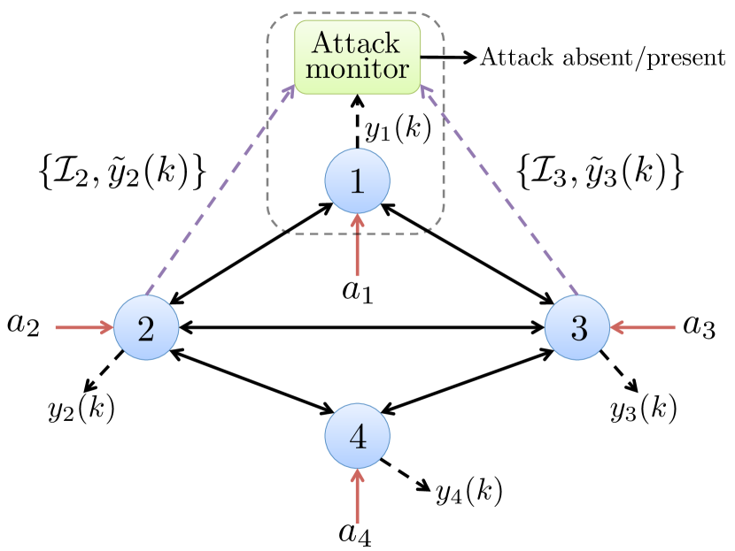
Each subsystem is equipped with an attack monitor whose goal is to detect the local attack using the local measurements. Since Subsystem $i$ does not know $B_{i}^{a}$ , it can only detect $a_{i}=B_{i}^{a}\tilde{a}_{i}$ . The detection procedure requires the knowledge of the statistical properties of $y_{i}$ which depend on the interconnection signal $x_{-i}$ . Since the subsystems do not have knowledge of the interconnection signals (c.f. Assumption 1), they share their measurements among each other to aid the local detection of attacks (see Fig. 1). The details of how these shared measurements are used for attack detection are presented in Section 3.

Refer to caption — Figure 1: An interconnected system consisting of $N=4$ subsystems. The solid lines represent state coupling among the subsystems. For attack detection by Subsystem $1$ , its neighboring agents $2$ and $3$ communicate their output information to $1$ (denoted by dashed lines). The attack monitor associated with Subsystem $1$ uses the received information and the local measurements to detect attacks.

While the shared measurements help in detecting local attacks, they can reveal sensitive information of the subsystems. For instance, some of the states/outputs of a subsystem may be confidential, which it may not be willing to share with other subsystems. To protect the privacy of such states/outputs, we propose a privacy mechanism $\mathcal{M}_{i}$ through which a subsystem limits the amount and quality of its shared measurements. Thus, instead of sharing the complete measurements in (4), Subsystem $i$ shares limited measurements (denoted as $\tilde{y}_{i}$ ) given by:

	$\displaystyle\mathcal{M}_{i}:\qquad\tilde{y}_{i}(k)$	$\displaystyle=S_{i}y_{i}(k)+\tilde{r}_{i}(k)$
		$\displaystyle=S_{i}C_{i}x_{i}(k)+S_{i}v_{i}(k)+\tilde{r}_{i}(k),$		(5)

where $S_{i}\in\mathbb{R}^{m_{i}\times p_{i}}$ is a selection matrix suitably chosen to select a subspace of the outputs, and $\tilde{r}_{i}(k)\sim\mathcal{N}(0,\Sigma_{\tilde{r}_{i}})$ is an artificial white noise (independent of $w_{i}$ and $v_{i}$ ) added to introduce additional inaccuracy in the shared measurements. Without loss of generality, we assume $S_{i}$ to be full row rank for all $i\in\mathcal{S}$ . Thus, a subsystem can limit its shared measurement via a combination of the following two mechanisms (i) by sharing fewer (or a subspace of) measurements, and (ii) by sharing more noisy measurements. Intuitively, when Subsystem $i$ limits its shared measurements, the estimates of its states/outputs computed by the other subsystems become more inaccurate. This prevents other subsystems from accurately determining the confidential states/outputs of Subsystem $i$ , thereby protecting its privacy. We will explain this phenomenon in detail in the next section.

Let the parameters corresponding to the limited measurements of subsystem $i$ be denoted by $\mathcal{I}_{i}\triangleq$
$\{C_{i},S_{i},\Sigma_{v_{i}},\Sigma_{\tilde{r}_{i}}\}$ . We make the following assumption:

Assumption 2: Each subsystem $i\in\mathcal{S}$ shares its limited measurements $\tilde{y}_{i}$ in (2) and the parameters $\mathcal{I}_{i}$ with all subsystems $j\in\mathcal{S}_{-i}.$ ¹¹1To be precise, this information sharing is required only between neighboring subsystems, i.e., between subsystems that are directly coupled with each other in (1). $\square$

Under Assumptions 1 and 2, the goal of each subsystem $i$ is to detect the local attack $a_{i}$ using its local measurements $y_{i}$ and the limited measurements $\{\tilde{y}_{j}\}_{j\in\mathcal{S}_{-i}}$ received from the other subsystems (see Fig. 1). Further, we are interested in characterizing the trade-off between the privacy level and the detection performance.

3 Local attack detection

In this section, we present the local attack detection procedure of the subsystems and characterize their detection performance. For the ease or presentation, we describe the analysis for Subsystem $1$ and remark that the procedure is analogous for the other subsystems.

3.1 Measurement collection

We employ a batch detection scheme in which each subsystem collects the measurements for $k=1,2,\cdots,T$ , with $T>0$ , and performs detection based on the collective measurements. In this subsection, we model the collected local and shared measurements for Subsystem $1$ .

Local measurements: Let the time-aggregated local measurements, interconnection signals, attacks, process noise and measurement noise corresponding to Subsystem $1$ be respectively denoted by

$\displaystyle y_{L}$	$\displaystyle\triangleq[y_{1}^{\mathsf{T}}(1),y_{1}^{\mathsf{T}}(2),\cdots,y_{1}^{\mathsf{T}}(T)]^{\mathsf{T}},$
$\displaystyle x$	$\displaystyle\triangleq[x_{-1}^{\mathsf{T}}(0),x_{-1}^{\mathsf{T}}(1),\cdots,x_{-1}^{\mathsf{T}}(T-1)]^{\mathsf{T}},$
$\displaystyle\tilde{a}$	$\displaystyle\triangleq[\tilde{a}_{1}^{\mathsf{T}}(0),\tilde{a}_{1}^{\mathsf{T}}(1),\cdots,\tilde{a}_{1}^{\mathsf{T}}(T-1)]^{\mathsf{T}},$
$\displaystyle w$	$\displaystyle\triangleq[w_{1}^{\mathsf{T}}(0),w_{1}^{\mathsf{T}}(1),\cdots,w_{1}^{\mathsf{T}}(T-1)]^{\mathsf{T}},$
$\displaystyle v$	$\displaystyle\triangleq[v_{1}^{\mathsf{T}}(1),v_{1}^{\mathsf{T}}(2),\cdots,v_{1}^{\mathsf{T}}(T)]^{\mathsf{T}},\quad\text{and let}$
$\displaystyle F(Z)$	$\displaystyle\triangleq\begin{bmatrix}C_{1}Z&0&\cdots&0\\ C_{1}A_{1}Z&C_{1}Z&\cdots&0\\ \vdots&\vdots&\ddots&\vdots\\ C_{1}A_{1}^{T-1}Z&C_{1}A_{1}^{T-2}Z&\cdots&C_{1}Z\end{bmatrix}$	(6)
	$\displaystyle=F(I)(I_{T}\otimes Z).$

By using (3) recursively and (4), the local measurements can be written as

$\displaystyle y_{L}$	$\displaystyle=Ox_{1}(0)+F_{x}x+F_{\tilde{a}}\tilde{a}+F_{w}w+v,$	(7)
$\displaystyle\text{where}\quad F_{x}$	$\displaystyle=F({B_{1}}),\>F_{\tilde{a}}=F(B_{1}^{a}),\>F_{w}=F(I),\quad\text{and}$
$\displaystyle O$	$\displaystyle\triangleq\begin{bmatrix}(C_{1}A_{1})^{\mathsf{T}}&(C_{1}A_{1}^{2})^{\mathsf{T}}&\cdots&(C_{1}A_{1}^{T})^{\mathsf{T}}\end{bmatrix}^{\mathsf{T}}.$

Note that $w\sim\mathcal{N}(0,\Sigma_{w})$ and $v\sim\mathcal{N}(0,\Sigma_{v})$ with

\displaystyle\Sigma_{w}=I_{T}\otimes\Sigma_{w_{1}}>0\quad\text{and}\quad\Sigma_{v}=I_{T}\otimes\Sigma_{v_{1}}>0.

Let $v_{L}\triangleq Ox_{1}(0)+F_{w}w+v$ denote the effective local noise in the measurement equation (7). Using the fact that $(x_{1}(0),w,v)$ are independent, the overall local measurements of the subsystem are given by

	$\displaystyle y_{L}$	$\displaystyle=F_{x}x+F_{\tilde{a}}\tilde{a}+v_{L},\quad\text{where}$		(8)
	$\displaystyle v_{L}$	$\displaystyle\sim\mathcal{N}(0,\Sigma_{v_{L}}),\>\Sigma_{v_{L}}=O\Sigma_{x_{1}(0)}O^{\mathsf{T}}+F_{w}\Sigma_{w}F_{w}^{\mathsf{T}}+\Sigma_{v}>0.$

Shared measurements: Let $\tilde{y}_{-1}(k)\triangleq$
$[\tilde{y}_{2}^{\mathsf{T}}(k),\tilde{y}_{3}^{\mathsf{T}}(k),\cdots,\tilde{y}_{N}^{\mathsf{T}}(k)]^{\mathsf{T}}$ denote the limited measurements received by Subsystem $1$ from all the other subsystems at time $k$ . Further, let $v_{-1}(k)$ and $\tilde{r}_{-1}(k)$ denote similar aggregated vectors of $\left\{v_{j}(k)\right\}_{j\in\mathcal{S}_{-1}}$ and $\left\{\tilde{r}_{j}(k)\right\}_{j\in\mathcal{S}_{-1}}$ , respectively. Then, from (2) we have

		$\displaystyle\tilde{y}_{-1}(k)=S_{-1}C_{-1}x_{-1}(k)+S_{-1}v_{-1}(k)+\tilde{r}_{-1}(k),$		(9)
		$\displaystyle\text{where}\>\>\>S_{-1}\!\triangleq\text{diag}(S_{2},\cdots,S_{N}),C_{-1}\!\triangleq\text{diag}(C_{2},\cdots,C_{N}),$
		$\displaystyle v_{-1}(k)\sim\mathcal{N}(0,\Sigma_{v_{-1}}),\>\Sigma_{v_{-1}}=\text{diag}(\Sigma_{v_{2}},\cdots,\Sigma_{v_{N}})>0,$
		$\displaystyle\tilde{r}_{-1}(k)\sim\mathcal{N}(0,\Sigma_{\tilde{r}_{-1}}),\>\Sigma_{\tilde{r}_{-1}}=\text{diag}(\Sigma_{\tilde{r}_{2}},\cdots,\Sigma_{\tilde{r}_{N}})\geq 0.$

Further, let the time-aggregated limited measurements received by Subsystem $1$ be denoted by $y_{R}\triangleq$
$[\tilde{y}_{-1}^{\mathsf{T}}(0),\tilde{y}_{-1}^{\mathsf{T}}(1),\cdots,\tilde{y}_{-1}^{\mathsf{T}}(T-1)]^{\mathsf{T}}$ , and let $v_{R}$ denote similar time-aggregated vector of $\left\{S_{-1}v_{-1}(k)+\tilde{r}_{-1}(k)\right\}_{k=0,\cdots,T-1}$ . Then, from (9), the overall limited measurements received by Subsystem $1$ read as

$\displaystyle y_{R}$	$\displaystyle=Hx+v_{R},\quad\text{where}$	(10)
$\displaystyle H$	$\displaystyle\triangleq I_{T}\otimes S_{-1}C_{-1},\quad\text{and}\quad v_{R}\sim\mathcal{N}(0,\Sigma_{v_{R}})$
$\displaystyle\text{with}\quad\Sigma_{v_{R}}$	$\displaystyle=I_{T}\otimes(S_{-1}\Sigma_{v_{-1}}S_{-1}^{\mathsf{T}}+\Sigma_{\tilde{r}_{-1}})>0.$

The goal of Subsystem $1$ is to detect the local attack using the local and received measurements given by (8) and (10), respectively.

3.2 Measurement processing

Since Subsystem $1$ does not have access to the interconnection signal $x$ , it uses the received measurements to obtain an estimate of $x$ . Note that Subsystem $1$ is oblivious to the statistics of the stochastic signal $x$ . Therefore, it computes an estimate of $x$ assuming that $x$ is a deterministic but unknown quantity.

According to (10), $y_{R}\sim\mathcal{N}(Hx,\Sigma_{v_{R}})$ , and the Maximum Likelihood (ML) estimate of $x$ based on $y_{R}$ is computed by maximizing the log-likelihood function of $y_{R}$ , and is given by:

	$\displaystyle{\hat{x}}$	$\displaystyle{=\arg\underset{z}{\max}\quad-\frac{1}{2}(y_{R}-Hz)^{\mathsf{T}}\Sigma_{v_{R}}^{-1}(y_{R}-Hz)}$
	$\displaystyle\begin{split}&\overset{{(a)}}{=}\tilde{H}^{+}H^{\mathsf{T}}\Sigma_{v_{R}}^{-1}y_{R}+(I-\tilde{H}^{+}\tilde{H})d,\quad\text{where}\\ \tilde{H}&\triangleq H^{\mathsf{T}}\Sigma_{v_{R}}^{-1}H\geq 0,\end{split}$			(11)

$d$ is any real vector of appropriate dimension, and equality $(a)$ follows from Lemma A.1 in the Appendix. If $\tilde{H}$ (or equivalently $H$ ) is not full column rank, then the estimate can lie anywhere in Null( $\tilde{H}$ ) = Null( $H$ ) (shifted by $\tilde{H}^{+}H^{\mathsf{T}}\Sigma_{v_{R}}^{-1}y_{R}$ ). Thus, the component of $x$ that lies in Null( $H$ ) cannot be estimated and only the component of $x$ that lies in Im( $\tilde{H}$ ) = Im( $H^{\mathsf{T}}$ ) can be estimated. Based on this discussion, we decompose $x$ as

$\displaystyle x$	$\displaystyle=(I-\tilde{H}^{+}\tilde{H})x+\tilde{H}^{+}\tilde{H}x$
	$\displaystyle=(I-\tilde{H}^{+}\tilde{H})x+\tilde{H}^{+}H^{\mathsf{T}}\Sigma_{v_{R}}^{-1}Hx$
	$\displaystyle\overset{\eqref{eq:share_meas_2}}{=}(I-\tilde{H}^{+}\tilde{H})x+\tilde{H}^{+}H^{\mathsf{T}}\Sigma_{v_{R}}^{-1}(y_{R}-v_{R}).$	(12)

Substituting $x$ from (12) in (8), we get

	$\displaystyle y_{L}$	$\displaystyle=F_{x}(I-\tilde{H}^{+}\tilde{H})x+F_{x}\tilde{H}^{+}H^{\mathsf{T}}\Sigma_{v_{R}}^{-1}(y_{R}-v_{R})$
		$\displaystyle+F_{\tilde{a}}\tilde{a}+v_{L}.$		(13)

Next, we process the local measurements in two steps. First, we subtract the known term $F_{x}\tilde{H}^{+}H^{\mathsf{T}}\Sigma_{v_{R}}^{-1}y_{R}$ . Second, we eliminate the component $(I-\tilde{H}^{+}\tilde{H})x$ (which cannot be estimated) by premultiplying (3.2) with a matrix $M^{\mathsf{T}}$ , where

	$\displaystyle M$	$\displaystyle=\text{Basis of Null}\left([F_{x}(I-\tilde{H}^{+}\tilde{H})]^{\mathsf{T}}\right),$
		$\displaystyle\Rightarrow M^{\mathsf{T}}F_{x}(I-\tilde{H}^{+}\tilde{H})=0.$		(14)

Since the columns of $M$ are basis vectors, $M$ is full column rank. The processed measurements are given by

	$\displaystyle z$	$\displaystyle=M^{\mathsf{T}}(y_{L}-F_{x}\tilde{H}^{+}H^{\mathsf{T}}\Sigma_{v_{R}}^{-1}y_{R})$
		$\displaystyle\overset{\eqref{eq:block_meas2},\eqref{eq:left_null_matrix}}{=}M^{\mathsf{T}}F_{\tilde{a}}\tilde{a}+\underbrace{M^{\mathsf{T}}(v_{L}-F_{x}\tilde{H}^{+}H^{\mathsf{T}}\Sigma_{v_{R}}^{-1}v_{R}),}_{\textstyle\triangleq v_{P}}$		(15)

where $v_{P}\sim\mathcal{N}(0,\Sigma_{v_{P}})$ . The random variables $v_{L}$ and $v_{R}$ are independent because they depend exclusively on the local and external subsystems’ noise, respectively. Using this fact

	$\displaystyle\Sigma_{v_{P}}$	$\displaystyle=M^{\mathsf{T}}\left[\Sigma_{v_{L}}+F_{x}\tilde{H}^{+}H^{\mathsf{T}}\Sigma_{v_{R}}^{-1}\Sigma_{v_{R}}\Sigma_{v_{R}}^{-\mathsf{T}}H(\tilde{H}^{+})^{\mathsf{T}}F_{x}^{\mathsf{T}}\right]M$
		$\displaystyle\overset{\tilde{H}^{\mathsf{T}}=\tilde{H}}{=}M^{\mathsf{T}}\Sigma_{v_{L}}M+M^{\mathsf{T}}F_{x}\tilde{H}^{+}F_{x}^{\mathsf{T}}M\overset{(a)}{>}0,$		(16)

where $(a)$ follows from the facts that $M$ is full column rank and $\Sigma_{v_{L}}>0$ . The processed measurements $z$ in (15) depend only on the local attack $\tilde{a}$ , and the Gaussian noise $v_{P}$ whose statistics is known to Subsystem $1$ (c.f. Assumptions 1 and 2), i.e. $z\sim\mathcal{N}(M^{\mathsf{T}}F_{\tilde{a}}\tilde{a},\Sigma_{v_{P}})$ . Thus, Subsystem $1$ uses $z$ to perform attack detection. Note that the attack vectors that belong to Null( $M^{\mathsf{T}}F_{\tilde{a}}$ ) cannot be detected.

The operation of elimination of the unknown component $(I-\tilde{H}^{+}\tilde{H})x$ from $y_{L}$ also eliminates a component of the attack $\tilde{a}$ . As a result, this operation increases the space of undetectable attack vectors from Null( $F_{\tilde{a}}$ ) to Null( $M^{\mathsf{T}}F_{\tilde{a}}$ ). In some cases, this operation could also result in complete elimination of attacks as shown in the next result.

Lemma 3.1

Consider equation (3) and the limited measurements in (2), and let $S_{-1},C_{-1},M$ be defined in (9) and (14). If

\displaystyle\textnormal{Im}(B_{1}^{a})\subseteq\textnormal{Im}\left({B_{1}}\left[I-(S_{-1}C_{-1})^{+}(S_{-1}C_{-1})\right]\right),

(17)

then $M^{\mathsf{T}}F_{\tilde{a}}=0$ .

Proof: Since Null( $\tilde{H}$ ) = Null( $H$ ), we have

\displaystyle\tilde{H}^{+}\tilde{H}=H^{+}H=I_{T}\otimes(S_{-1}C_{-1})^{+}(S_{-1}C_{-1}).

Let $Z\triangleq(S_{-1}C_{-1})^{+}(S_{-1}C_{-1})$ . Then, substituting $F_{x}$ from (7) in (14), we get

	$\displaystyle M^{\mathsf{T}}F(I)(I_{T}\otimes{B_{1}})[I-I_{T}\otimes Z]=0$
$\displaystyle\Rightarrow$	$\displaystyle M^{\mathsf{T}}F(I)(I_{T}\otimes{B_{1}})[I_{T}\otimes(I-Z)]=0$
$\displaystyle\Rightarrow$	$\displaystyle M^{\mathsf{T}}F(I)(I_{T}\otimes{B_{1}}[I-Z])=0.$	(18)

If (17) holds, then there exists a matrix $P$ such that $B_{1}^{a}={B_{1}}[I-Z]P$ . Thus, from (7), we have

	$\displaystyle M^{\mathsf{T}}F_{\tilde{a}}$	$\displaystyle=M^{\mathsf{T}}F(I)(I_{T}\otimes{B_{1}}[I-Z]P)$
		$\displaystyle=M^{\mathsf{T}}F(I)(I_{T}\otimes{B_{1}}[I-Z])(I_{T}\otimes P)\overset{\eqref{eq:undet_attack_pf_1}}{=}0.$

The above result has the following intuitive interpretation: if the attacks lie in the subspace of the interconnections that cannot be estimated, then eliminating these interconnections also eliminates the attacks. In this case, the processed measurements do not have any signature of the attacks, which, therefore, cannot be detected. This result highlights the limitation of our measurement processing procedure. Next, we illustrate the result using an example.

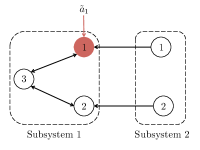
Example 1

Consider an interconnected subsystem consisting of two subsystems with the following parameters (see Fig. 2):

\displaystyle\small A_{1}=\begin{bmatrix}1&0&-1\\ 0&1&-1\\ 1&1&1\end{bmatrix},\>\>{B_{1}}=\begin{bmatrix}1&0\\ 0&1\\ 0&0\end{bmatrix},\>\>B_{1}^{a}=\begin{bmatrix}1\\ 0\\ 0\end{bmatrix},

$C_{1}=I_{3},C_{2}=I_{2}$ and $T=1$ . We have $F_{x}={B_{1}}$ and $F_{\tilde{a}}=B_{1}^{a}$ . Consider the following two cases:
Case (i): Subsystem $2$ shares its 2nd state, i.e., $S_{2}=S_{-1}=\begin{bmatrix}0&1\end{bmatrix}$ . In this case, Subsystem $1$ does not get information about the interconnection affecting its 1st state and the elimination of this interconnection also eliminates the attack. It can be verified that $M=\left[\begin{smallmatrix}0&1&0\\ 0&0&1\end{smallmatrix}\right]^{\mathsf{T}}$ and $M^{\mathsf{T}}B_{1}^{a}=0$ .
Case (ii): Subsystem $2$ shares its 1st state, i.e., $S_{2}=S_{-1}=\begin{bmatrix}1&0\end{bmatrix}$ . In this case, Subsystem $1$ gets information about the interconnection affecting its 1st state. Thus, its elimination is not required and this preserves the attack. It can be verified that $M=\left[\begin{smallmatrix}1&0&0\\ 0&0&1\end{smallmatrix}\right]^{\mathsf{T}}$ and $M^{\mathsf{T}}B_{1}^{a}\neq 0$ .

3.3 Statistical hypothesis testing

The goal of Subsystem $1$ is to determine whether it is under attack or not using the processed measurements $z$ in (15). Recall that, since Subsystem 1 does not know $B_{1}^{a}$ , it can only detect $a_{1}=B_{1}^{a}\tilde{a}_{1}$ . Let $a\triangleq$
$[(B_{1}^{a}\tilde{a}_{1}(0))^{\mathsf{T}},\cdots,(B_{1}^{a}\tilde{a}_{1}(T-1))^{\mathsf{T}}]^{\mathsf{T}}$ . Then, from (7), we have $F_{\tilde{a}}\tilde{a}=F_{a}a$ , where $F_{a}=F(I)$ . Thus, processed measurements are distributed according to $z\sim\mathcal{N}(M^{\mathsf{T}}F_{a}a,\Sigma_{v_{P}})$ . We cast the attack detection problem as a binary hypothesis testing problem. Since Subsystem $1$ does not know the attack $a$ , we consider the following composite (simple vs. composite) testing problem

	$\displaystyle H_{0}:\quad a=0\quad\text{(Attack absent)}\qquad\text{vs}$
	$\displaystyle H_{1}:\quad a\neq 0\quad\text{(Attack present)}$

We use the Generalized Likelihood Ratio Test (GLRT) criterion [36] for the above testing problem, which is given by

	$\displaystyle\frac{f(z\|H_{0})}{\underset{a}{\sup}f(z\|H_{1})}\overset{H_{0}}{\underset{H_{1}}{\gtrless}}\tau^{\prime}\quad\text{where,}$	(19)
$\displaystyle f(z\|H_{0})$	$\displaystyle=\frac{1}{\sqrt{2\pi\|\Sigma_{v_{P}}\|}}e^{-\frac{1}{2}z^{\mathsf{T}}\Sigma_{v_{P}}^{-1}z}\quad\text{and,}$
$\displaystyle f(z\|H_{1})$	$\displaystyle=\frac{1}{\sqrt{2\pi\|\Sigma_{v_{P}}\|}}e^{-\frac{1}{2}(z-M^{\mathsf{T}}F_{a}a)^{\mathsf{T}}\Sigma_{v_{P}}^{-1}(z-M^{\mathsf{T}}F_{a}a)},$

are the probability density functions of the multivariate Gaussian distribution of $z$ under hypothesis $H_{0}$ and $H_{1}$ , respectively, and $\tau^{\prime}$ is a suitable threshold. Using the result in Lemma A.1 in the Appendix to compute the denominator in (19) and taking the logarithm, the test (19) can be equivalently written as

	$\displaystyle t(z)$	$\displaystyle\triangleq z^{\mathsf{T}}\Sigma_{v_{P}}^{-1}M^{\mathsf{T}}F_{a}\tilde{M}^{+}F_{a}^{\mathsf{T}}M\Sigma_{v_{P}}^{-1}z\overset{H_{1}}{\underset{H_{0}}{\gtrless}}\tau,$		(20)
	where	$\displaystyle\quad\tilde{M}=F_{a}^{\mathsf{T}}M\Sigma_{v_{P}}^{-1}M^{\mathsf{T}}F_{a},$

and $\tau\geq 0$ is the threshold. The above test is a $\chi^{2}$ test since the test statistics $t(z)$ follows a chi-squared distribution (see Lemma 3.3). The next result simplifies the test statistics $t(z)$ and provides an interpretation of the test.

Lemma 3.2

(Simplification of test statistics) Let $\Sigma_{v_{P}}^{-1}=R^{\mathsf{T}}R$ denote the Cholesky decomposition of $\Sigma_{v_{P}}^{-1}$ . Then,

\displaystyle\Sigma_{v_{P}}^{-1}M^{\mathsf{T}}F_{a}\tilde{M}^{+}F_{a}^{\mathsf{T}}M\Sigma_{v_{P}}^{-1}=R^{\mathsf{T}}UU^{\mathsf{T}}R,

(21)

where $U$ is a matrix whose columns are the orthonormal basis vectors of $\textnormal{Im}(RM^{\mathsf{T}}F_{a})$ .

Proof: Let $M_{1}\triangleq M^{\mathsf{T}}F_{a}$ . Then

\displaystyle\tilde{M}^{+}=(M_{1}^{\mathsf{T}}R^{\mathsf{T}}RM_{1})^{+}=(RM_{1})^{+}((RM_{1})^{+})^{\mathsf{T}}.

Thus, we have

	$\displaystyle\Sigma_{v_{P}}^{-1}$	$\displaystyle M^{\mathsf{T}}F_{a}\tilde{M}^{+}F_{a}^{\mathsf{T}}M\Sigma_{v_{P}}^{-1}$
		$\displaystyle=(R^{\mathsf{T}}R)M_{1}(RM_{1})^{+}((RM_{1})^{+})^{\mathsf{T}}M_{1}^{\mathsf{T}}(R^{\mathsf{T}}R)$
		$\displaystyle=R^{\mathsf{T}}(RM_{1})(RM_{1})^{+}(RM_{1})(RM_{1})^{+}R$
		$\displaystyle=R^{\mathsf{T}}(RM_{1})(RM_{1})^{+}R.$

Since $RM_{1}(RM_{1})^{+}$ is the orthogonal projection operator on $\text{Im}(RM_{1})$ , $RM_{1}(RM_{1})^{+}=UU^{\mathsf{T}}$ , and the proof is complete.

Using Lemma 3.2, the test (20) can be written as

\displaystyle t(z)=z^{\mathsf{T}}R^{\mathsf{T}}UU^{\mathsf{T}}Rz\overset{H_{1}}{\underset{H_{0}}{\gtrless}}\tau.

(22)

Thus, the test compares the energy of the signal $U^{\mathsf{T}}Rz$ with a given threshold to detect the attacks. Next, we derive the distribution of the test statistics under both hypothesis.

Lemma 3.3

(Distribution of test statistics) The distribution of test statistics $t(z)$ in (22) is given by

	$\displaystyle t(z)$	$\displaystyle\sim\chi_{q}^{2}\quad\text{under $H_{0}$},$		(23)
	$\displaystyle t(z)$	$\displaystyle\sim\chi_{q}^{2}(\lambda\triangleq a^{\mathsf{T}}\Lambda a)\quad\text{under $H_{1}$},$		(24)

where $q=\textnormal{Rank}(M^{\mathsf{T}}F_{a})$ and $\Lambda=F_{a}^{\mathsf{T}}M\Sigma_{v_{P}}^{-1}M^{\mathsf{T}}F_{a}$ .

Proof: By the definition of $U$ in (21), and recalling $\Sigma_{v_{P}}^{-1}=R^{\mathsf{T}}R$ with $R$ being non-singular, we have

\displaystyle\text{Rank}(U^{\mathsf{T}}U)=\text{Rank}(U)=\text{Rank}(RM^{\mathsf{T}}F_{a})=\text{Rank}(M^{\mathsf{T}}F_{a}).

Let $z^{\prime}=U^{\mathsf{T}}Rz$ . Under $H_{0}$ , $z\sim\mathcal{N}(0,\Sigma_{v_{P}})$ . Thus,

\displaystyle z^{\prime}\sim\mathcal{N}(0,U^{\mathsf{T}}R\Sigma_{v_{P}}R^{\mathsf{T}}U)\overset{(a)}{=}\mathcal{N}(0,I_{q}),

where $(a)$ follows from $R\Sigma_{v_{P}}R^{\mathsf{T}}=I$ and $U^{\mathsf{T}}U=I_{q}$ . Therefore, $t(z)=(z^{\prime})^{\mathsf{T}}z^{\prime}\sim\chi_{q}^{2}$ .

Let $M_{1}=M^{\mathsf{T}}F_{a}$ . Under $H_{1}$ , $z\sim\mathcal{N}(M_{1}a,\Sigma_{v_{P}})$ . Thus,

	$\displaystyle z^{\prime}$	$\displaystyle\sim\mathcal{N}(U^{\mathsf{T}}RM_{1}a,I_{q})$
	$\displaystyle\Rightarrow t(z)=(z^{\prime})^{\mathsf{T}}z^{\prime}$	$\displaystyle\sim\chi_{q}^{2}(a^{\mathsf{T}}M_{1}^{\mathsf{T}}R^{T}UU^{\mathsf{T}}RM_{1}a).$

Using $UU^{\mathsf{T}}=RM_{1}(RM_{1})^{+}$ from the proof of Lemma 3.2, we have

	$\displaystyle a^{\mathsf{T}}M_{1}^{\mathsf{T}}R^{T}UU^{\mathsf{T}}RM_{1}a=a^{\mathsf{T}}(RM_{1})^{\mathsf{T}}(RM_{1})(RM_{1})^{+}(RM_{1})a$
	$\displaystyle=a^{\mathsf{T}}(RM_{1})^{\mathsf{T}}(RM_{1})a=a^{\mathsf{T}}M_{1}^{\mathsf{T}}\Sigma_{v_{P}}^{-1}M_{1}a=\lambda,$

and the proof is complete.

Remark 2

(Interpretation of detection parameters $(q,\lambda)$ ) The parameter $q$ denotes the number of independent observations of the attack vector $a$ in the processed measurements (15). The parameter $\lambda$ can be interpreted as the signal to noise ratio (SNR) of the processed measurements in (15), where the signal of interest is the attack. $\square$

Next, we characterize the performance of the test (20). Let the probability of false alarm and probability of detection for the test be respectively denoted by

	$\displaystyle P_{F}$	$\displaystyle=\text{Prob}(t(z)>\tau\|H_{0})\overset{(a)}{=}\mathcal{Q}_{q}(\tau)\quad\text{and,}$
	$\displaystyle P_{D}$	$\displaystyle=\text{Prob}(t(z)>\tau\|H_{1})\overset{(b)}{=}\mathcal{Q}_{q}(\tau;\lambda),$

where $(a)$ and $(b)$ follow from (23) and (24), respectively. Recall that $\mathcal{Q}_{q}(x)$ and $\mathcal{Q}_{q}(x;\lambda)$ denote the right tail probabilities of chi-square and noncentral chi-square distributions, respectively. Inspired by the Neyman-Pearson test framework, we select the size ( $P_{F}$ ) of the test and determine the threshold $\tau$ which provides the desired size. Then, we use the threshold to perform the test and compute the detection probability. Thus, we have

	$\displaystyle\tau(q,P_{F})$	$\displaystyle=\mathcal{Q}_{q}^{-1}(P_{F}),$		(25)
	$\displaystyle P_{D}(q,\lambda,P_{F})$	$\displaystyle=\mathcal{Q}_{q}(\tau(q,P_{F});\lambda).$		(26)

The arguments in $\tau(q,P_{F})$ and $P_{D}(q,\lambda,P_{F})$ explicitly denote the dependence of these quantities on the detection parameters $(q,\lambda)$ and the probability of false alarm ( $P_{F}$ ). Note that the detection performance of Subsystem $1$ is characterized by the pair $(P_{F},P_{D})$ , where a lower value of $P_{F}$ and a higher value of $P_{D}$ is desirable. Later, in order to compare the performance of two different tests, we select a common value of $P_{F}$ for both of them, and then compare the detection probability $P_{D}$ .

The next result states the dependence of the detection probability on the detection parameters $(q,\lambda)$ .

Lemma 3.4

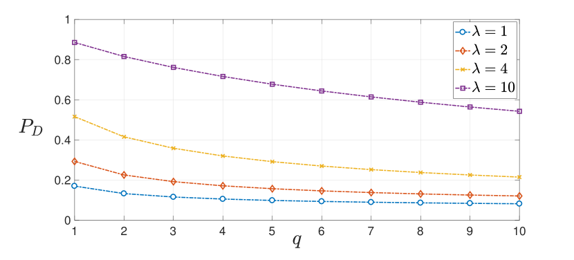
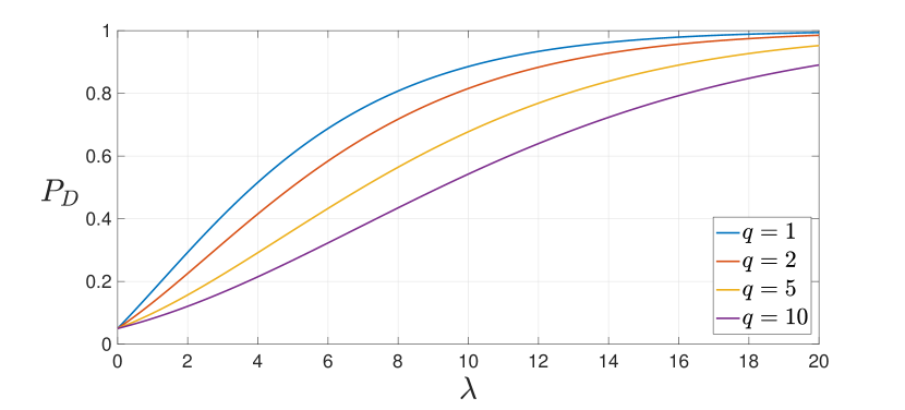
(Dependence of detection performance on detection parameters $(q,\lambda)$ ) For any given false alarm probability $P_{F}$ , the detection probability $P_{D}(q,\lambda,P_{F})$ is decreasing in $q$ and increasing in $\lambda$ .

Proof: Since $P_{F}$ is fixed, we omit it in the notation. It is a standard result that for a fixed $q$ (and $\tau(q)$ ), the CDF $(=1-\mathcal{Q}_{q}(\tau(q);\lambda)=1-P_{D}(q,\lambda))$ of a noncentral chi-square random variable is decreasing in $\lambda$ [37]. Thus, $P_{D}(q,\lambda)$ is increasing in $\lambda$ .

Next, we have [37]

\displaystyle P_{D}(q,\lambda)=e^{-\lambda/2}\sum_{j=0}^{\infty}\frac{(\lambda/2)^{j}}{j!}\mathcal{Q}_{q+2j}(\tau(q)).

From [38, Corollary 3.1], it follows that $\mathcal{Q}_{q+2j}(\tau(q))=\mathcal{Q}_{q+2j}(\mathcal{Q}_{q}^{-1}(P_{F}))$ is decreasing in $q$ for all $j>0$ . Thus, $P_{D}(q,\lambda)$ is decreasing in $q$ .

Figure 3 illustrates the dependence of the detection probability on the parameters $(q,\lambda)$ . Lemma 3.4 implies that for a fixed $q$ , a higher SNR ( $\lambda$ ) leads to a better detection performance, which is intuitive. However, for a fixed $\lambda$ , an increase in the number of independent observations ( $q$ ) results in degradation of the detection performance. This counter-intuitive behavior is due to the fact that the GLRT in (19) is not an uniformly most powerful (UMP) test for all values of the attack $a$ . In fact, a UMP test does not exist in this case [39]. Thus, the test can perform better for some particular attack values while it may not perform as good for other attack values. This suboptimality is an inherent property of the GLRT in (19). It arises due to the composite nature of the test and the fact that the value of the attack vector $a$ is not known to the attack monitor.

Remark 3

(Composite vs. simple test) If the value of the attack vector (say $a_{1}$ ) is known, we can cast a simple (simple vs. simple) binary hypothesis testing problem as $H_{0}:a=0$ vs. $H_{1}:a=a_{1}$ and use the standard Likelihood Ratio Test criterion for detection. In this case the detection probability depends only on $P_{F}$ and SNR $(\lambda)$ , and for any given $P_{F}$ , the detection performance improves as the SNR increases. $\square$

4 Privacy quantification

In this section, we quantify the privacy of the mechanism $\mathcal{M}_{i}$ in (2) in terms of the estimation error covariance of the state $x_{i}$ . For simplicity, we assume $i\neq 1$ , and this estimation is performed by Subsystem $1$ , which is directly coupled with Subsystem $i$ and receives limited measurements from it. Then, we use this quantification to compare and rank different privacy mechanisms.

We use a batch estimation scheme in which the estimate is computed based on the collective measurements obtained for $k=0,1,\cdots,T-1$ , with $T>0$ . Let $\tilde{y}_{i}=[\tilde{y}_{i}^{\mathsf{T}}(0),\cdots,\tilde{y}_{i}^{\mathsf{T}}(T-1)]^{\mathsf{T}}$ , and let $x_{i}$ , $v_{i}$ , $\tilde{r}_{i}$ be similar time-aggregated vectors of $x_{i}(k),v_{i}(k),\tilde{r}_{i}(k)$ , respectively. Then, using (2), we have

\displaystyle\tilde{y}_{i}=(\underbrace{I_{T}\otimes S_{i}C_{i}}_{\textstyle\triangleq H_{i}})x_{i}+\underbrace{(I_{T}\otimes S_{i})v_{i}+\tilde{r}_{i}}_{\textstyle\triangleq r_{i}},

(27)

where $r_{i}\sim\mathcal{N}(0,\Sigma_{r_{i}})$ with $\Sigma_{r_{i}}=I_{T}\otimes(S_{i}\Sigma_{v_{i}}S_{i}^{\mathsf{T}}+\Sigma_{\tilde{r}_{i}})$ . Note that Subsystem $1$ that receives measurements (27) from Subsystem $i$ knows $\{H_{i},\Sigma_{r_{i}}\}$ (c.f. Assumption 2). However, it is oblivious to the statistics of the confidential stochastic signal $x_{i}$ . Therefore, it computes an estimate of $x_{i}$ assuming that $x_{i}$ is a deterministic but unknown quantity. Further, this estimate is computed by Subsystem $1$ using the measurements received only from Subsystem $i$ , and it does not use its local measurements or the measurements received from other subsystems for this purpose. The reason is twofold. First, although the local measurements $y_{L}$ of Subsystem $1$ depend on $x_{i}$ due to the interconnected nature of the system (see (8)), they cannot be used due to the presence of the unknown attack on Subsystem $1$ given by $F_{\tilde{a}}\tilde{a}=F_{a}a$ , where $F_{a}=F(I)$ is known and $a$ is unknown. If we try to eliminate these unknown attacks by pre-multiplying (8) with a matrix $M^{\prime}$ , where $(M^{\prime})^{\mathsf{T}}$ is the basis of Null( $F_{a}$ ), this operation also eliminates $x$ (and $x_{i}$ ), since $\text{Null}(F_{a})\subseteq\text{Null}(F_{x})$ . Second, the measurements received from other subsystems cannot be used since Subsystem $1$ does not have the knowledge of the dynamics or attacks on these other subsystems.²²2Due to these reasons, the estimation capability of any Subsystem $j\in\mathcal{S}_{-i}$ trying to infer $x_{i}$ will be the same.

According to (27), $\tilde{y}_{i}\sim\mathcal{N}(H_{i}x_{i},\Sigma_{r_{i}})$ , and the Maximum Likelihood (ML) estimate of $x_{i}$ based on $\tilde{y}_{i}$ is computed by maximizing the log-likelihood function of $\tilde{y}_{i}$ , and is given by:

	$\displaystyle{\hat{x}_{i}}$	$\displaystyle{=\arg\underset{z}{\max}\quad-\frac{1}{2}(\tilde{y}_{i}-H_{i}z)^{\mathsf{T}}\Sigma_{r_{i}}^{-1}(\tilde{y}_{i}-H_{i}z)}$
	$\displaystyle\begin{split}&\overset{{(a)}}{=}\tilde{H}_{i}^{+}H_{i}^{\mathsf{T}}\Sigma_{r_{i}}^{-1}\tilde{y}_{i}+(I-\tilde{H}_{i}^{+}\tilde{H}_{i})d_{i},\quad\text{where}\\ \tilde{H}_{i}&\triangleq H_{i}^{\mathsf{T}}\Sigma_{r_{i}}^{-1}H_{i}\geq 0,\end{split}$			(28)

$d_{i}$ is any real vector of appropriate dimension, and equality $(a)$ follows from Lemma A.1 in the Appendix. If $\tilde{H}_{i}$ (or equivalently $H_{i}$ ) is not full column rank, then the estimate can lie anywhere in Null( $\tilde{H}_{i}$ ) = Null( $H_{i}$ ) (shifted by $\tilde{H}_{i}^{+}H_{i}^{\mathsf{T}}\Sigma_{r_{i}}^{-1}\tilde{y}_{i}$ ). Thus, the component of $x_{i}$ that lies in Null( $H_{i}$ ) cannot be estimated and only the component of $x_{i}$ that lies in Im( $\tilde{H}_{i}$ ) = Im( $H_{i}^{\mathsf{T}}$ ) can be estimated. Let $\mathcal{P}_{i}\triangleq\tilde{H}_{i}^{+}\tilde{H}_{i}$ denote the projection operator on Im( $\tilde{H}_{i}$ ). The estimation error in this subspace is given by:

	$\displaystyle e_{i}$	$\displaystyle=\mathcal{P}_{i}x_{i}-\mathcal{P}_{i}\hat{x}_{i}=\tilde{H}_{i}^{+}\tilde{H}_{i}x_{i}-\tilde{H}_{i}^{+}H_{i}^{\mathsf{T}}\Sigma_{r_{i}}^{-1}\tilde{y}_{i}$
		$\displaystyle=-\tilde{H}_{i}^{+}H_{i}^{\mathsf{T}}\Sigma_{r_{i}}^{-1}r_{i},$		(29)

and the estimation error covariance is given by:

	$\displaystyle\Sigma_{e_{i}}$	$\displaystyle=\mathbb{E}[\tilde{H}_{i}^{+}H_{i}^{\mathsf{T}}\Sigma_{r_{i}}^{-1}r_{i}r_{i}^{\mathsf{T}}\Sigma_{r_{i}}^{-1}H_{i}\tilde{H}_{i}^{+}]$
		$\displaystyle{=\tilde{H}_{i}^{+}\underbrace{H_{i}^{\mathsf{T}}\Sigma_{r_{i}}^{-1}H_{i}}_{\tilde{H}_{i}}\tilde{H}_{i}^{+}}=\tilde{H}_{i}^{+}.$		(30)

Note that since the model in (27) is linear with Gaussian noise, $\mathcal{P}_{i}\hat{x}_{i}$ is the minimum-variance unbiased (MVU) estimate of $x_{i}$ projected on Im( $H_{i}^{\mathsf{T}}$ ). Thus, the covariance $\Sigma_{e_{i}}$ captures the fundamental limit on how accurately $\mathcal{P}_{i}x_{i}$ can be estimated and, therefore, it is a suitable metric to quantify privacy.

The privacy level of mechanism $\mathcal{M}_{i}$ in (2) is characterized by two quantities: (i) rank( $S_{i}$ ), and (ii) $\Sigma_{e_{i}}$ . Intuitively, if rank( $S_{i}$ ) is small, then Subsystem $i$ shares fewer measurements and, as a result, the component of $x_{i}$ that cannot be estimated $((I-\tilde{H}_{i}^{+}\tilde{H}_{i})x_{i})$ becomes large. Further, if $\Sigma_{e_{i}}$ is large (in a positive semi-definite sense), this implies that the estimation accuracy of the component of $x_{i}$ that can be estimated $(\tilde{H}_{i}^{+}\tilde{H}_{i}x_{i})$ is worse. Thus, a lower value of rank( $S_{i}$ ) and a larger value of $\Sigma_{e_{i}}$ implies a larger level of privacy. Based on this discussion, we next define an ordering between two privacy mechanisms.

Consider two privacy mechanisms $\mathcal{M}_{i}^{(1)}$ and $\mathcal{M}_{i}^{(2)}$ , and let $\tilde{y}_{i}^{(k)},\hat{x}_{i}^{(k)}$ , $k=1,2$ denote the limited measurements and estimates corresponding to the two mechanisms, respectively. Further, let $S_{i}^{(k)},H_{i}^{(k)},\tilde{H}_{i}^{(k)},\mathcal{P}_{i}^{(k)},\Sigma_{e_{i}}^{(k)},$ $k=1,2$ denote the quantities defined above corresponding to $\mathcal{M}_{i}^{(1)}$ and $\mathcal{M}_{i}^{(2)}$ .

Definition 1

(Privacy ordering) Mechanism $\mathcal{M}_{i}^{(2)}$ is more private than $\mathcal{M}_{i}^{(1)}$ , denoted by $\mathcal{M}_{i}^{(2)}\geq\mathcal{M}_{i}^{(1)}$ , if

\displaystyle\begin{split}&(i)\>\textnormal{Im}\left((S_{i}^{(2)})^{\mathsf{T}}\right)\subseteq\textnormal{Im}\left((S_{i}^{(1)})^{\mathsf{T}}\right)\quad\text{and,}\hskip 50.0pt\\ &(ii)\>\Sigma_{e_{i}}^{(2)}\geq\mathcal{P}_{i}^{(2)}\Sigma_{e_{i}}^{(1)}\mathcal{P}_{i}^{(2)}.\hskip 105.0pt\hbox{$\square$}\end{split}

(31)

The first condition implies that $\tilde{y}_{i}^{(2)}$ is a limited version of $\tilde{y}_{i}^{(1)}$ and is required for the ordering to be well defined. Under this condition, it is easy to see that $\text{Im}(H_{i}^{(2)})=\text{Im}(\mathcal{P}_{i}^{(2)})\subseteq\text{Im}(H_{i}^{(1)})=\text{Im}(\mathcal{P}_{i}^{(1)})$ . Thus, the estimated component $\mathcal{P}_{i}^{(2)}\hat{x}_{i}^{(2)}$ lies in a subspace that is contained in the subspace of the estimated component $\mathcal{P}_{i}^{(1)}\hat{x}_{i}^{(1)}$ . For a fair comparison between the two mechanisms, we consider the projection of $\mathcal{P}_{i}^{(1)}\hat{x}_{i}^{(1)}$ on $\text{Im}(\mathcal{P}_{i}^{(2)})$ , given by
$\mathcal{P}_{i}^{(2)}\mathcal{P}_{i}^{(1)}\hat{x}_{i}^{(1)}=\mathcal{P}_{i}^{(2)}\hat{x}_{i}^{(1)}$ . Then, we compare its estimation error (given by $\mathcal{P}_{i}^{(2)}\Sigma_{e_{i}}^{(1)}\mathcal{P}_{i}^{(2)}$ ) with the estimation error of $\mathcal{P}_{i}^{(2)}\hat{x}_{i}^{(2)}$ (given by $\Sigma_{e_{i}}^{(2)}$ ) to obtain the second condition in (31). Next, we present an example to illustrate Definition 1.

Example 2

Let $x_{i}\in\mathbb{R}^{2}$ , $C_{i}=I_{2}$ , $T=1$ , and consider two privacy mechanisms given by:

	$\displaystyle\mathcal{M}_{i}^{(1)}:\qquad\qquad\tilde{y}_{i}^{(1)}=(x_{i}+v_{i})+\tilde{r}_{i}^{(1)},$
	$\displaystyle\mathcal{M}_{i}^{(2)}:\qquad\qquad\tilde{y}_{i}^{(2)}=\begin{bmatrix}1&0\end{bmatrix}(x_{i}+v_{i})+\tilde{r}_{i}^{(2)},$

with $\Sigma_{v_{i}}=\Sigma_{\tilde{r}_{i}}^{(1)}=I_{2}$ and $\Sigma_{\tilde{r}_{i}}^{(2)}=\alpha\geq 0$ . Mechanism $\mathcal{M}_{i}^{(1)}$ shares both components of the measurement vector $y_{i}$ ( $S_{i}^{(1)}=I_{2}$ ) whereas $\mathcal{M}_{i}^{(2)}$ shares only the first component ( $S_{i}^{(2)}=[1\>\>0]$ ), and both add some artificial noise. The state estimates under the two mechanisms (using (28)) are given by

\displaystyle\hat{x}_{i}^{(1)}=\tilde{y}_{i}^{(1)}\quad\text{and}\quad\hat{x}_{i}^{(2)}=\left[\begin{matrix}1\\ 0\end{matrix}\right]\tilde{y}_{i}^{(2)}+\left[\begin{matrix}0&0\\ 0&1\end{matrix}\right]d_{i}.

Thus, under $\mathcal{M}_{i}^{(1)}$ both components of $x_{i}$ can be estimated while under $\mathcal{M}_{i}^{(2)}$ , only the first component can be estimated. Further, we have $\Sigma_{e_{i}}^{(1)}=2I_{2},\Sigma_{e_{i}}^{(2)}=\left[\begin{smallmatrix}1+\alpha&0\\ 0&0\end{smallmatrix}\right]$ and $\mathcal{P}_{i}^{(2)}=\left[\begin{smallmatrix}1&0\\ 0&0\end{smallmatrix}\right]$ . Thus, the estimation error covariance of the first component of $x_{i}$ under $\mathcal{M}_{i}^{(1)}$ and $\mathcal{M}_{i}^{(2)}$ are $2$ and $1+\alpha$ , respectively, and $\mathcal{M}_{i}^{(2)}$ is more private than $\mathcal{M}_{i}^{(1)}$ if $\alpha\geq 1$ .

On the other hand, if $\alpha<1$ , then an ordering between the mechanisms cannot be established. In this case, under $\mathcal{M}_{i}^{(1)}$ , both the state components can be estimated but the estimation error in first component is large. In contrast, under $\mathcal{M}_{i}^{(2)}$ , only the first component can be estimated but its estimation error is small. $\square$

Next, we state a sufficient condition on the noise added by two privacy mechanisms that guarantee the ordering of the mechanisms. This condition implies that, if one privacy mechanism shares a subspace of the measurements of the other mechanism and injects a sufficiently large amount of noise, then it is more private.

Lemma 4.1

(Sufficient condition for privacy ordering) Consider two privacy mechanisms $\mathcal{M}_{i}^{(1)}$ and $\mathcal{M}_{i}^{(2)}$ in (2) with parameters $(S_{i}^{(k)},\Sigma_{\tilde{r}_{i}}^{(k)})$ , $k=1,2$ that satisfy condition $(i)$ of (31). Let $P$ be a full row rank matrix that satisfies $S_{i}^{(2)}=PS_{i}^{(1)}$ . If

\displaystyle\Sigma_{\tilde{r}_{i}}^{(2)}\geq P\Sigma_{\tilde{r}_{i}}^{(1)}P^{\mathsf{T}},

(32)

then $\mathcal{M}_{i}^{(2)}$ is more private than $\mathcal{M}_{i}^{(1)}$ .

Proof: From (27) and (28), we have

\displaystyle\tilde{H}_{i}^{(k)}=I_{T}\otimes\underbrace{(S_{i}^{(k)}C_{i})^{\mathsf{T}}\left[S_{i}^{(k)}\Sigma_{v_{i}}(S_{i}^{(k)})^{\mathsf{T}}+\Sigma_{\tilde{r}_{i}}^{(k)}\right]^{-1}S_{i}^{(k)}C_{i}}_{\triangleq Y^{(k)}}.

Since $(S_{i}^{(1)},S_{i}^{(2)})$ satisfy (31) $(i)$ , there always exist a full row rank matrix $P$ satisfying $S_{i}^{(2)}=PS_{i}^{(1)}$ . Next we have,

		$\displaystyle Y^{(2)}\!\!=\!(S_{i}^{(1)}C_{i})^{\mathsf{T}}P^{\mathsf{T}}\!\left[PS_{i}^{(1)}\Sigma_{v_{i}}(S_{i}^{(1)})^{\mathsf{T}}P^{\mathsf{T}}\!+\!\Sigma_{\tilde{r}_{i}}^{(2)}\right]^{-1}\!\!PS_{i}^{(1)}C_{i}$
		$\displaystyle=\!(S_{i}^{(1)}C_{i})^{\mathsf{T}}\!P^{\mathsf{T}}\!\left[\!P(S_{i}^{(1)}\Sigma_{v_{i}}(S_{i}^{(1)})^{\mathsf{T}}\!\!+\!\Sigma_{\tilde{r}_{i}}^{(1)})P^{\mathsf{T}}\!\!+\!E\right]^{-1}\!\!\!PS_{i}^{(1)}C_{i}$
		$\displaystyle\overset{(a)}{\leq}\!\!(S_{i}^{(1)}C_{i})^{\mathsf{T}}\!\!\left[S_{i}^{(1)}\Sigma_{v_{i}}(S_{i}^{(1)})^{\mathsf{T}}\!\!+\!\Sigma_{\tilde{r}_{i}}^{(1)}\right]^{-1}\!\!\!S_{i}^{(1)}C_{i}=Y^{(1)}$		(33)

where $E\triangleq\Sigma_{\tilde{r}_{i}}^{(2)}-P\Sigma_{\tilde{r}_{i}}^{(1)}P^{\mathsf{T}}$ and $(a)$ follows from $E\geq 0$ (using (32)) and Lemma A.3 in the Appendix. From (4), it follows that

	$\displaystyle\tilde{H}_{i}^{(2)}\leq\tilde{H}_{i}^{(1)}\overset{(b)}{\Rightarrow}\tilde{H}_{i}^{(2)}\geq\tilde{H}_{i}^{(2)}(\tilde{H}_{i}^{(1)})^{+}\tilde{H}_{i}^{(2)}$
	$\displaystyle\overset{(c)}{\Rightarrow}(\tilde{H}_{i}^{(2)})^{+}\tilde{H}_{i}^{(2)}(\tilde{H}_{i}^{(2)})^{+}\geq(\tilde{H}_{i}^{(2)})^{+}\tilde{H}_{i}^{(2)}(\tilde{H}_{i}^{(1)})^{+}\tilde{H}_{i}^{(2)}(\tilde{H}_{i}^{(2)})^{+}$
	$\displaystyle\overset{(d)}{=}\text{Condition $(ii)$ in \eqref{eq:priv_order}},$

where $(b)$ follows from [40, Lemma 1], and $(c)$ , $(d)$ follow from facts that $(\tilde{H}_{i}^{(k)})^{+}$ is symmetric and $(\tilde{H}_{i}^{(k)})^{+}\tilde{H}_{i}^{(k)}=\tilde{H}_{i}^{(k)}(\tilde{H}_{i}^{(k)})^{+}$ . Thus, both conditions in (31) are satisfied and $\mathcal{M}_{i}^{(2)}\geq\mathcal{M}_{i}^{(1)}$ .

We conclude this section by showing that the privacy mechanism in (2) exhibits an intuitive post-processing property. It implies that if we further limit the measurements produced by a privacy mechanism, then this operation cannot decrease the privacy of the measurements. This post-processing property also holds in the differential privacy framework [26].

Lemma 4.2

(Post-processing increases privacy) Consider two privacy mechanisms $\mathcal{M}_{i}^{(1)}$ and $\mathcal{M}_{i}^{(2)}$ , where $\mathcal{M}_{i}^{(2)}$ further limits the measurements of $\mathcal{M}_{i}^{(1)}$ as:

	$\displaystyle\mathcal{M}_{i}^{(1)}:\qquad\tilde{y}_{i}^{(1)}(k)$	$\displaystyle=S_{i}^{(1)}y_{i}(k)+\tilde{r}_{i}^{(1)}(k)$
	$\displaystyle\mathcal{M}_{i}^{(2)}:\qquad\tilde{y}_{i}^{(2)}(k)$	$\displaystyle=S\tilde{y}_{i}^{(1)}(k)+n_{i}(k),$

where $S$ is full row rank and $n_{i}(k)\sim\mathcal{N}(0,\Sigma_{n_{i}})$ . Then, $\mathcal{M}_{i}^{(2)}$ is more private than $\mathcal{M}_{i}^{(1)}$ .

Proof: It is easy to observe that $S_{i}^{(2)}=SS_{i}^{(1)}$ and $\tilde{r}_{i}^{(2)}(k)=S\tilde{r}_{i}^{(1)}(k)+n_{i}(k)$ . Thus,

\displaystyle\Sigma_{\tilde{r}_{i}}^{(2)}=S\Sigma_{\tilde{r}_{i}}^{(1)}S^{\mathsf{T}}+\Sigma_{n_{i}}\geq S\Sigma_{\tilde{r}_{i}}^{(1)}S^{\mathsf{T}},

and the result follows from Lemma 4.1.

Remark 4

(Comparison with Differential Privacy (DP)) Additive noise based privacy mechanisms have also been proposed in the framework of DP. Specifically, the notion of $(\epsilon,\delta)$ -DP uses a zero-mean Gaussian noise [26]. Although the frameworks of DP and this paper use additive Gaussian noises, there are conceptual differences between the two. The DP framework distinguishes between the cases when a single subsystem is present or absent in the system, and tries to make the output statistically similar in both the cases. It allows access to arbitrary side information and does not involve any specific estimation algorithm. In contrast, our privacy framework assumes no side information and privacy guarantees are specific to the considered estimation procedure. Moreover, besides adding noise, our framework also allows for an additional means to vary privacy by sending fewer measurements, which is not feasible in the DP framework. $\square$

5 Detection performance vs privacy trade-off

In this section, we present a trade-off between the attack detection performance and privacy of the subsystems. As before, we focus on detection for Subsystem $1$ and consider two measurement sharing privacy mechanisms $\mathcal{M}_{j}^{(1)}$ and $\mathcal{M}_{j}^{(2)}$ for all other subsystems $j\in\mathcal{S}_{-1}$ . The trade-off is between the detection performance of Subsystem 1 and the privacy level of all other subsystems. We begin by characterizing the relation between the detection parameters corresponding to these two sets of privacy mechanisms.

Theorem 5.1

(Relation among the detection parameters of privacy mechanisms) Let $\mathcal{M}_{j}^{(2)}$ be more private than $\mathcal{M}_{j}^{(1)}$ for all $j\in\mathcal{S}_{-1}$ . Given any attack vector $a$ , let $q^{(k)}$ and $\lambda^{(k)}=a^{\mathsf{T}}{\Lambda}^{(k)}a$ denote the detection parameters under the privacy mechanisms $\left\{\mathcal{M}_{j}^{(k)}\right\}_{j\in\mathcal{S}_{-1}}$ , for $k=1,2$ . Then, we have

\displaystyle\begin{split}&(i)\>q^{(1)}\geq q^{(2)}\quad\text{and,}\hskip 130.0pt\\ &(ii)\>\lambda^{(2)}\mu_{max}\geq\lambda^{(1)}\geq\lambda^{(2)}\mu_{min}\geq\lambda^{(2)},\end{split}

(34)

where $\mu_{max}$ and $\mu_{min}$ are the largest and smallest generalized eigenvalues of $({\Lambda}^{(1)},{\Lambda}^{(2)})$ , respectively.

Proof: From (2), (9) and (10), for $k=1,2$ , we have

	$\displaystyle H^{(k)}$	$\displaystyle=I_{T}\otimes\text{diag}\left(S_{2}^{(k)}C_{2},\cdots,S_{N}^{(k)}C_{N}\right)=S_{-1}^{(k)}H,$
	$\displaystyle\Sigma_{v_{R}}^{(k)}$	$\displaystyle=S_{-1}^{(k)}\Sigma_{v_{R}}(S_{-1}^{(k)})^{\mathsf{T}}+\Sigma_{\tilde{r}_{-1}}^{(k)}>0\quad\text{where,}$
	$\displaystyle S_{-1}^{(k)}$	$\displaystyle=I_{T}\otimes\text{diag}\left(S_{2}^{(k)},\cdots,S_{N}^{(k)}\right),$
	$\displaystyle\Sigma_{\tilde{r}_{-1}}^{(k)}$	$\displaystyle=I_{T}\otimes\text{diag}\left(\Sigma_{\tilde{r}_{2}}^{(k)},\cdots,\Sigma_{\tilde{r}_{N}}^{(k)}\right)\geq 0.$

Since $\mathcal{M}_{j}^{(2)}\geq\mathcal{M}_{j}^{(1)}$ for all $j\in\mathcal{S}_{-1}$ , the first condition in (31) results in

\displaystyle\text{Im}\!\left(\!(S_{-1}^{(1)})^{\mathsf{T}}\right)\!\!\supseteq\!\text{Im}\!\left(\!(S_{-1}^{(2)})^{\mathsf{T}}\right)\!\Rightarrow\!\text{Im}\!\left(\!(H^{(1)})^{\mathsf{T}}\right)\!\!\supseteq\!\text{Im}\!\left(\!(H^{(2)})^{\mathsf{T}}\right).

From (11), we have $\tilde{H}^{(k)}=(H^{(k)})^{\mathsf{T}}(\Sigma_{v_{R}}^{(k)})^{-1}H^{(k)}$ . Since $\text{Null}(\tilde{H}^{(k)})=\text{Null}(H^{(k)})$ , from (14), it follows that
$\text{Im}(M^{(1)})\supseteq\text{Im}(M^{(2)})$ . Recalling from (24) that $q^{(k)}=\text{Rank}((M^{(k)})^{\mathsf{T}}F_{a})$ , it follows that $q^{(1)}\geq q^{(2)}$ .

Since $\text{Im}(M^{(1)})\supseteq\text{Im}(M^{(2)})$ , we have $M^{(2)}=M^{(1)}P$ for some full column rank matrix $P$ . Let $Z\triangleq F_{x}^{\mathsf{T}}M^{(1)}P$ . From (16), we have

	$\displaystyle\Sigma_{v_{P}}^{(2)}$	$\displaystyle=(M^{(2)})^{\mathsf{T}}\Sigma_{v_{L}}M^{(2)}+(M^{(2)})^{\mathsf{T}}F_{x}(\tilde{H}^{(2)})^{+}F_{x}^{\mathsf{T}}M^{(2)},$
		$\displaystyle=P^{\mathsf{T}}\Sigma_{v_{P}}^{(1)}P+\underbrace{Z^{\mathsf{T}}[(\tilde{H}^{(2)})^{+}-(\tilde{H}^{(1)})^{+}]Z}_{\triangleq E}.$		(35)

Next, we show that $E\geq 0$ . . Using $M^{(2)}=M^{(1)}P$ , and using (14) for both $\{M^{(k)},\tilde{H}^{(k)}\}$ , $k=1,2$ , we have

\displaystyle Z^{\mathsf{T}}(\tilde{H}^{(1)})^{+}\tilde{H}^{(1)}=Z^{\mathsf{T}}(\tilde{H}^{(2)})^{+}\tilde{H}^{(2)}.

(36)

Thus, we get

		$\displaystyle E=Z^{\mathsf{T}}[(\tilde{H}^{(2)})^{+}-(\tilde{H}^{(1)})^{+}\tilde{H}^{(1)}(\tilde{H}^{(1)})^{+}\tilde{H}^{(1)}(\tilde{H}^{(1)})^{+}]Z$
		$\displaystyle=\!Z^{\mathsf{T}}[(\tilde{H}^{(2)})^{+}\!\!-\!(\tilde{H}^{(2)})^{+}\!\tilde{H}^{(2)}(\tilde{H}^{(1)})^{+}\!(\tilde{H}^{(2)})^{+}\!\tilde{H}^{(2)}]Z$		(37)

where the last inequality follows from (36) and the fact that $\tilde{H}^{(k)}(\tilde{H}^{(k)})^{+}=(\tilde{H}^{(k)})^{+}\tilde{H}^{(k)}$ . Next, we have,


		$\displaystyle\tilde{H}^{(k)}\!=\!I_{T}\!\otimes\!\text{diag}\Big{[}\!(S_{2}^{(k)}C_{2})^{\mathsf{T}}\!(S_{2}^{(k)}\Sigma_{v_{2}}(S_{2}^{(k)})^{\mathsf{T}}\!\!+\!\Sigma_{\tilde{r}_{2}}^{(k)})^{-1}\!S_{2}^{(k)}C_{2},$
		$\displaystyle\cdots,(S_{N}^{(k)}C_{N})^{\mathsf{T}}\left(S_{N}^{(k)}\Sigma_{v_{N}}(S_{N}^{(k)})^{\mathsf{T}}+\Sigma_{\tilde{r}_{N}}^{(k)}\right)^{-1}S_{N}^{(k)}C_{N}\Big{]}$
		$\displaystyle\!=\!\Pi^{\mathsf{T}}\text{diag}\Big{[}\!I_{T}\!\otimes\!(S_{2}^{(k)}C_{2})^{\mathsf{T}}(S_{2}^{(k)}\Sigma_{v_{2}}(S_{2}^{(k)})^{\mathsf{T}}\!\!+\!\Sigma_{\tilde{r}_{2}}^{(k)})^{-1}S_{2}^{(k)}C_{2},$
		$\displaystyle\cdots,I_{T}\!\otimes\!(S_{N}^{(k)}C_{N})^{\mathsf{T}}\!\left(\!S_{N}^{(k)}\Sigma_{v_{N}}(S_{N}^{(k)})^{\mathsf{T}}\!+\!\Sigma_{\tilde{r}_{N}}^{(k)}\right)^{-1}\!S_{N}^{(k)}C_{N}\Big{]}\Pi$
		$\displaystyle=\Pi^{\mathsf{T}}\text{diag}\left[\tilde{H}_{2}^{(k)},\cdots,\tilde{H}_{N}^{(k)}\right]\Pi\quad\text{and,}$		(38a)
		$\displaystyle(\tilde{H}^{(k)})^{+}=\Pi^{\mathsf{T}}\text{diag}\left[(\tilde{H}_{2}^{(k)})^{+},\cdots,(\tilde{H}_{N}^{(k)})^{+}\right]\Pi,$		(38b)

where $\Pi$ is a permutation matrix with $\Pi^{-1}=\Pi^{\mathsf{T}}$ . Substituting (38a) and (38b) in (5), we have

	$\displaystyle E$	$\displaystyle=Z^{\mathsf{T}}\Pi^{\mathsf{T}}\text{diag}\Big{[}(\tilde{H}_{2}^{(2)})^{+}-\mathcal{P}_{2}^{(2)}(\tilde{H}_{2}^{(1)})^{+}\mathcal{P}_{2}^{(2)},\cdots$
		$\displaystyle(\tilde{H}_{N}^{(2)})^{+}-\mathcal{P}_{N}^{(2)}(\tilde{H}_{N}^{(1)})^{+}\mathcal{P}_{N}^{(2)}\Big{]}\Pi Z\overset{(a)}{\geq}0,$

where $(a)$ follows from the second condition in (31) for all $j\in\mathcal{S}_{-1}$ . Next, from (24), we have,

	$\displaystyle\Lambda^{(2)}$	$\displaystyle=F_{a}^{\mathsf{T}}M^{(2)}(\Sigma_{v_{P}}^{(2)})^{-1}(M^{(2)})^{\mathsf{T}}F_{a}$
		$\displaystyle\overset{\eqref{eq:det_par_comp_pf_0}}{=}F_{a}^{\mathsf{T}}M^{(1)}\underbrace{P(P^{\mathsf{T}}\Sigma_{v_{P}}^{(1)}P+E)^{-1}P^{\mathsf{T}}}_{\triangleq Y}(M^{(1)})^{\mathsf{T}}F_{a}$
		$\displaystyle\overset{(b)}{\leq}F_{a}^{\mathsf{T}}M^{(1)}(\Sigma_{v_{P}}^{(1)})^{-1}(M^{(1)})^{\mathsf{T}}F_{a}=\Lambda^{(1)},$
	$\displaystyle\Rightarrow\lambda^{(1)}$	$\displaystyle=a^{\mathsf{T}}\Lambda^{(1)}a\geq a^{\mathsf{T}}\Lambda^{(2)}a=\lambda^{(2)},$

where $(b)$ follows from Lemma A.3 in the Appendix, and the facts that $E\geq 0$ and $P$ is full column rank. Finally, the second condition in (34) follows from Lemma A.4 in the Appendix, and the proof is complete.

Theorem 5.1 shows that when the subsystems $j\in\mathcal{S}_{-1}$ share measurements with Subsystem $1$ using more private mechanisms, both the number of processed measurements and the SNR reduce. This has implications on the detection performance of Subsystem $1$ , as explained next. To compare the performance corresponding to the two sets of privacy mechanisms, we select the same false alarm probability $P_{F}$ for both the cases and compare the detection probability. Theorem 5.1 and Lemma 3.4 imply that $P_{D}(q^{(2)},\lambda^{(2)},P_{F})$ can be greater or smaller than $P_{D}(q^{(1)},\lambda^{(1)},P_{F})$ depending on the actual values of the detection parameters. In fact, ignoring the dependency on $P_{F}$ since it is same for both cases, we have

	$\displaystyle P_{D}(q^{(2)},\lambda^{(2)})-P_{D}(q^{(1)},\lambda^{(1)})=$
	$\displaystyle\!\underbrace{P_{D}(q^{(2)}\!,\lambda^{(2)}\!)\!-\!P_{D}(q^{(2)}\!,\lambda^{(1)}\!)}_{\leq 0}+\underbrace{P_{D}(q^{(2)}\!,\lambda^{(1)}\!)\!-\!P_{D}(q^{(1)}\!,\lambda^{(1)}\!).}_{\geq 0}$

Intuitively, if the decrease in $P_{D}$ due to the decrease in the SNR³³3Note that the SNR depends upon the attack vector $a$ (via (24)), which we do not know a-priori. Thus, depending on the actual attack value, the SNR can take any positive value. ( $\lambda^{(1)}\rightarrow\lambda^{(2)}$ ) is larger than the increase in $P_{D}$ due to the decrease in the number of measurements ( $q^{(1)}\rightarrow q^{(2)}$ ), then the the detection performance decreases, and vice-versa. The next result formalizes this intuition.

Theorem 5.2

(Condition for trade-off) Consider the setup in Theorem 5.1, and let the detection probability be given in (26). Then, for a given $P_{F}$ , a security-privacy trade-off exists if and only if

\displaystyle P_{D}(q^{(2)},\lambda^{(2)},P_{F})\leq P_{D}(q^{(1)},\lambda^{(1)},P_{F}).

The above result presents an analytical condition for the trade-off. When this condition is violated, a counter trade-off exists. This is an interesting and counter-intuitive trade-off between the detection performance and privacy/ information sharing, and it implies that, in certain cases, sharing less information can lead to a better detection performance. This phenomenon occurs because the GLRT for the considered hypothesis testing problem is a sub-optimal test, as discussed before.

5.1 Privacy using only noise

In this subsection, we analyze the special case when the subspace of the shared measurements is fixed, and the privacy level can be varied by changing only the noise level. We begin by comparing the detection performance corresponding to two privacy mechanisms that share the same subspace of measurements.

Corollary 5.3

(Strict security-privacy trade-off ) Consider two privacy mechanisms $\mathcal{M}_{j}^{(2)}\geq\mathcal{M}_{j}^{(1)}$ such that $\textnormal{Im}\left((S_{j}^{(2)})^{\mathsf{T}}\right)=\textnormal{Im}\left((S_{j}^{(1)})^{\mathsf{T}}\right)$ for $j\in\mathcal{S}_{-1}$ . Let ( $q^{(k)},\lambda^{(k)}$ ) denote the detection parameters of Subsystem 1 under the privacy mechanisms $\left\{\mathcal{M}_{j}^{(k)}\right\}_{j\in\mathcal{S}_{-1}}$ , for $k=1,2$ . Then, for any given $P_{F}$ , we have

\displaystyle P_{D}(q^{(2)},\lambda^{(2)},P_{F})\leq P_{D}(q^{(1)},\lambda^{(1)},P_{F}).

Proof: Since the mechanisms share the same subspace of measurements, from the proof of Theorem 5.1, we have

	$\displaystyle\text{Im}\!\left(\!(S_{-1}^{(1)})^{\mathsf{T}}\right)\!\!$	$\displaystyle=\!\text{Im}\!\left(\!(S_{-1}^{(2)})^{\mathsf{T}}\right)\!\Rightarrow\!\text{Im}\!\left(\!(H^{(1)})^{\mathsf{T}}\right)\!\!=\!\text{Im}\!\left(\!(H^{(2)})^{\mathsf{T}}\right)$
		$\displaystyle\Rightarrow\!\text{Im}\!\left(\!M^{(1)}\right)\!\!=\!\text{Im}\!\left(\!M^{(2)}\right)\Rightarrow q^{(1)}=q^{(2)}.$

The fact that $\lambda^{(1)}\geq\lambda^{(2)}$ follows from Theorem 5.1, and the result then follows from Lemma 3.4.

The above result implies that there is strict trade-off between privacy and detection performance when the subspace of the shared measurements is fixed and the privacy level is varied by changing the noise level. In this case, more private mechanisms result in a poorer detection performance, and vice-versa.

Corollary 5.3 qualitatively captures the security-privacy trade-off. Next, we present a quantitative analysis that determines the best possible detection performance subject to a given privacy level. Note that since the subspace of the shared measurements is fixed, the detection parameter $q$ is also fixed, as well as $P_{F}$ and the attack $a$ . Thus, according to Lemma 3.4, the detection performance can be improved by increasing $\lambda=a^{\mathsf{T}}\Lambda a$ . Intuitively, $\lambda$ is large (irrespective of $a$ ) if $\Lambda$ is large, or when $\Lambda^{+}$ is small (in a positive-semidefinite sense).⁴⁴4Minimization of $\Lambda^{+}$ allows us to formulate a semidefinite optimization problem, as we show later. Further, the privacy level is quantified by the error covariance in (30). Based on this, we formulate the following optimization problem:⁵⁵5This problem corresponds to Subsystem $1$ . A similar problem can be formulated for the whole system whose cost is the sum of the costs of the individual subsystems.

		$\displaystyle\underset{\textstyle\Sigma_{\tilde{r}_{2}}\geq 0,\cdots,\Sigma_{\tilde{r}_{N}}\geq 0}{\min}$	$\displaystyle\text{Tr}(\Lambda^{+})$		(39)
		s.t.	$\displaystyle\text{Tr}(\Sigma_{e_{i}})\geq\epsilon_{i}^{\prime},\quad i=2,\cdots,N,$

where $\epsilon_{i}^{\prime}>0$ is the minimum desired privacy level of Subsystem $i$ . The design variables of the above optimization problem are the positive semi-definite noise covariance matrices $\Sigma_{\tilde{r}_{2}},\cdots,\Sigma_{\tilde{r}_{N}}$ . Next, we show that under some mild assumptions, (39) is a semidefinite optimization problem.

Lemma 5.4

Assume that $F(I)$ in (6) and $C_{i}$ for $i=1,\cdots,N$ are full row rank. Let $D_{1}=\sum_{i=1}^{T}D_{1,i}$ , where the matrices $D_{1,i}\in\mathbb{R}^{n_{1}\times n_{1}}$ , $i=1,\cdots,T$ are the block diagonal elements of $(M^{\mathsf{T}}F_{a})^{+}M^{\mathsf{T}}F_{a}$ . Further, let

	$\displaystyle K_{1}$	$\displaystyle=B_{1}(S_{-1}C_{-1})^{+},\qquad L_{1}=K_{1}^{\mathsf{T}}D_{1}K_{1},$
	$\displaystyle l_{1}$	$\displaystyle=\textnormal{Tr}\left[(M^{\mathsf{T}}F_{a})^{+}M^{\mathsf{T}}\Sigma_{v_{L}}M((M^{\mathsf{T}}F_{a})^{+})^{\mathsf{T}}\right]$
		$\displaystyle+\textnormal{Tr}\left[(M^{\mathsf{T}}F_{a})^{+}M^{\mathsf{T}}F_{a}\left[I_{T}\otimes\left(K_{1}S_{-1}\Sigma_{v_{-1}}S_{-1}^{\mathsf{T}}K_{1}^{\mathsf{T}}\right)\right]\right],$
	$\displaystyle g_{i}$	$\displaystyle=\textnormal{Tr}\left[H_{i}^{+}[I_{T}\otimes(S_{i}\Sigma_{v_{i}}S_{i}^{\mathsf{T}})](H_{i}^{+})^{\mathsf{T}}\right],$
	$\displaystyle G_{i}$	$\displaystyle=((S_{i}C_{i})^{+})^{\mathsf{T}}(S_{i}C_{i})^{+}.$

Then, $\textnormal{Tr}(\Lambda^{+})=l_{1}+\textnormal{Tr}(L_{1}\Sigma_{\tilde{r}_{-1}})$ and $\textnormal{Tr}(\Sigma_{e_{i}})=g_{i}+T\>\textnormal{Tr}(G_{i}\Sigma_{\tilde{r}_{i}})$ , where $\Sigma_{\tilde{r}_{-1}}=\textnormal{diag}(\Sigma_{\tilde{r}_{2}},\cdots,\Sigma_{\tilde{r}_{N}})$ .

Proof: From (30), $\Sigma_{e_{i}}=\tilde{H}_{i}^{+}$ , where $\tilde{H}_{i}=H_{i}^{\mathsf{T}}\Sigma_{r_{i}}^{-1}H_{i}$ and $H_{i}=I_{T}\otimes S_{i}C_{i}$ . Since, $S_{i}$ and $C_{i}$ are assumed to be full row rank, $H_{i}$ is full row rank. Next, we have

	$\displaystyle\tilde{H}_{i}^{+}$	$\displaystyle\overset{(a)}{=}H_{i}^{+}\Sigma_{r_{i}}(H_{i}^{+})^{\mathsf{T}}$
		$\displaystyle\overset{\eqref{eq:limited_meas_tag}}{=}\underbrace{H_{i}^{+}[I_{T}\otimes(S_{i}\Sigma_{v_{i}}S_{i}^{\mathsf{T}})](H_{i}^{+})^{\mathsf{T}}}_{U_{i}}+H_{i}^{+}[I_{T}\otimes\Sigma_{\tilde{r}_{i}}](H_{i}^{+})^{\mathsf{T}}$
		$\displaystyle\overset{\eqref{eq:limited_meas_tag}}{=}U_{i}+I_{T}\otimes[(S_{i}C_{i})^{+}\Sigma_{\tilde{r}_{i}}((S_{i}C_{i})^{+})^{\mathsf{T}}]$
		$\displaystyle\Rightarrow\textnormal{Tr}(\tilde{H}_{i}^{+})=g_{i}+T\>\textnormal{Tr}(G_{i}\Sigma_{\tilde{r}_{i}}),$

where $(a)$ follows from Lemma A.5 in the Appendix.

Next, from (24), $\Lambda=M_{1}^{\mathsf{T}}\Sigma_{v_{P}}^{-1}M_{1}$ where $M_{1}=M^{\mathsf{T}}F_{a}$ . Since $M^{\mathsf{T}}$ and $F_{a}=F(I)$ are assumed to be full row rank, $M_{1}$ is full row rank. Next, we have

	$\displaystyle\Lambda^{+}$	$\displaystyle\overset{(b)}{=}M_{1}^{+}\Sigma_{v_{P}}(M_{1}^{+})^{\mathsf{T}}$
		$\displaystyle\overset{\eqref{eq:z_noise_var},\eqref{eq:block_meas},(b)}{=}M_{1}^{+}M^{\mathsf{T}}\Sigma_{v_{L}}M(M_{1}^{+})^{\mathsf{T}}$
		$\displaystyle+M_{1}^{+}M_{1}(I_{T}\otimes B_{1})H^{+}\Sigma_{v_{R}}(H^{+})^{\mathsf{T}}(I_{T}\otimes B_{1}^{\mathsf{T}})M_{1}^{\mathsf{T}}(M_{1}^{+})^{\mathsf{T}}$
		$\displaystyle\overset{\eqref{eq:share_meas_2}}{=}M_{1}^{+}M^{\mathsf{T}}\Sigma_{v_{L}}M(M_{1}^{+})^{\mathsf{T}}$
		$\displaystyle+M_{1}^{+}M_{1}\left[I_{T}\otimes\left(K_{1}S_{-1}\Sigma_{v_{-1}}S_{-1}^{\mathsf{T}}K_{1}^{\mathsf{T}}\right)\right]M_{1}^{+}M_{1}$
		$\displaystyle+M_{1}^{+}M_{1}\left[I_{T}\otimes\left(K_{1}\Sigma_{\tilde{r}_{-1}}K_{1}^{\mathsf{T}}\right)\right]M_{1}^{+}M_{1},$
	$\displaystyle\Rightarrow$	$\displaystyle\textnormal{Tr}(\Lambda^{+})\overset{(c)}{=}l_{1}+\textnormal{Tr}(D_{1}K_{1}\Sigma_{\tilde{r}_{-1}}K_{1}^{\mathsf{T}})=l_{1}+\textnormal{Tr}(L_{1}\Sigma_{\tilde{r}_{-1}}).$

where $(b)$ follows from Lemma A.5 in the Appendix, and $(c)$ follows from the definition of $D_{1}$ and trivial algebraic manipulation.

Using the above theorem, (39) is equivalent to the following semidefinite optimization problem [41]

		$\displaystyle\underset{\textstyle\Sigma_{\tilde{r}_{2}}\geq 0,\cdots,\Sigma_{\tilde{r}_{N}}\geq 0}{\min}$	$\displaystyle\text{Tr}(L_{1}\Sigma_{\tilde{r}_{-1}})+l_{1}$		(40)
		s.t.	$\displaystyle\text{Tr}(G_{i}\Sigma_{\tilde{r}_{i}})\geq\frac{\epsilon_{i}^{\prime}-g_{i}}{T}:=\epsilon_{i}\geq 0,$

for $i=2,3,\cdots,N$ , which can be solved using standard semidefinite optimization algorithms [41]. This analysis allows us to design optimal noisy privacy mechanisms.

6 Simulation Example

We consider a power network model of the IEEE 39-bus test case [42] consisting of $10$ generators interconnected by transmission lines whose resistances are assumed to be negligible. Each generator is modeled according to the following second-order swing equation [43]:

\displaystyle M_{i}\ddot{\theta_{i}}+D_{i}\dot{\theta_{i}}=P_{i}-\sum_{k=1}^{n}\frac{E_{i}E_{k}}{X_{ik}}\sin(\theta_{i}-\theta_{k}),

(41)

where $\theta_{i},M_{i},D_{i},E_{i}$ and $P_{i}$ denote the rotor angle, moment of inertia, damping coefficient, internal voltage and mechanical power input of the $i^{\text{th}}$ generator, respectively. Further, $X_{ij}$ denotes the reactance of the transmission line connecting generators $i$ and $j$ ( $X_{ij}=\infty$ if they are not connected). We linearize (41) around an equilibrium point to obtain the following collective small-signal model:

\displaystyle\begin{bmatrix}d\dot{\theta}\\ d\ddot{\theta}\end{bmatrix}

\displaystyle=\underbrace{\begin{bmatrix}0&I\\ -M^{-1}L&-M^{-1}D\end{bmatrix}}_{\tilde{A}_{c}}\underbrace{\begin{bmatrix}d\theta\\ d\dot{\theta}\end{bmatrix}}_{\tilde{x}(t)}+\underbrace{\begin{bmatrix}0\\ M^{-1}B\end{bmatrix}}_{\tilde{B}^{a}_{c}}\tilde{a}(t),

(42)

where $d\theta$ denotes a small deviation of $\theta=\begin{bmatrix}\theta_{1}&\theta_{2}&\cdots&\theta_{10}\end{bmatrix}^{T}$ from the equilibrium value, $M=\text{diag}(M_{1},M_{2},\cdots,M_{10})$ , $D=\text{diag}(D_{1},D_{2},\cdots,D_{10})$ , and $L$ is a symmetric Laplacian matrix given by

\displaystyle L_{ij}=\begin{cases}-\frac{E_{i}E_{j}}{X_{ij}}\cos(\theta_{i}-\theta_{j})\quad&\text{for}\quad i\neq j,\\ -\sum\limits_{\begin{subarray}{c}j=1\\ j\neq i\end{subarray}}^{n}L_{ij}\quad&\text{for}\quad i=j.\end{cases}

(43)

Further, $\tilde{a}$ models small malicious alterations (attacks) in the mechanical power input of the generators that need to be detected. We assume that generators $\{1,4,8\}$ are under attack. Thus, $B=\begin{bmatrix}{\bf e_{1},e_{4},e_{8}}\end{bmatrix}$ , where ${\bf e_{j}}$ denotes the $j^{\text{th}}$ canonical vector. We assume that the power network is divided into 3 subsystems consisting of generators $\{1,2,3\}$ , $\{4,5,6,7\}$ and $\{8,9,10\}$ . Accordingly, we permute the state vector in (42) using a permutation matrix $\Pi$ such that $\Pi\tilde{x}=x=[x_{1}^{\mathsf{T}},x_{2}^{\mathsf{T}},x_{3}^{\mathsf{T}}]^{\mathsf{T}}$ , where $x_{i}$ consists of rotor angles and velocities of all generators in Subsystem $i$ . The transformed system is given by $\dot{x}=A_{c}x+B_{c}^{a}\tilde{a}(t)$ , where $A_{c}=\Pi\tilde{A}_{c}\Pi^{-1}$ and $B^{a}_{c}=\Pi\tilde{B}^{a}_{c}$ . Next, we sample this continuous time system with sampling time $T_{s}=0.1$ to obtain a discrete-time system $x(k+1)=Ax(k)+B^{a}\tilde{a}(k)$ with $A=e^{A_{c}T_{s}}$ and $B^{a}=\left(\int\limits_{t=0}^{T_{s}}e^{A_{c}\tau}d\tau\right)B_{c}^{a}$ . We assume that the discrete-time process dynamics are affected by process noise according to (1). The rotor angle and the angular velocity of all generators are measured using Phasor Measurement Units (PMUs) according to the noisy model (2). The time horizon is $T=3$ .

The generator voltage and angle values are obtained from [42]. We fix the damping coefficient for each generator as $10$ , and the moment of inertia values are chosen as $M=[70,10,40,30,70,30,90,80,40,50]$ . The reactance matrix $X$ is generated randomly, where each entry of $X$ is distributed independently according to $\mathcal{N}(0,0.01)$ . We focus on the attack detection for Subsystem $1$ , where Subsystems $2$ and $3$ use privacy mechanisms to share their measurements with Subsystem 1. The parameters of Subsystem 1 can be extracted from $A,B^{a}$ as $A=\begin{bmatrix}A_{1}\>\;B_{1}\\ *\end{bmatrix}$ and $B^{a}=\text{blockdiag}(B_{1}^{a},*,*)$ . The noise covariances are $\Sigma_{w_{1}}=0.5I_{6}$ and $\Sigma_{v_{1}}=\Sigma_{v_{3}}=I_{4}$ and $\Sigma_{v_{2}}=0.5I_{6}$ .

We consider the following three cases of privacy mechanisms for Subsystems 2 and 3:

(i)

$\mathcal{M}^{(0)}=\{\mathcal{M}_{2}^{(0)},\mathcal{M}_{3}^{(0)}\}$ : Subsystems 2 and 3 do not use any privacy mechanisms and share actual measurements, i.e., $S_{2}=I_{8},S_{3}=I_{6},\Sigma_{\tilde{r}_{2}}=0$ , and $\Sigma_{\tilde{r}_{3}}=0$ .
(ii)

$\mathcal{M}^{(1)}$ : Subsystem 2 does not use any privacy mechanism ( $S_{2}=I_{8},\Sigma_{\tilde{r}_{2}}=0$ ) while Subsystem 3 shares noisy measurements of generators $\{8,9\}$
( $S_{3}=\left[{\bf e_{1},e_{2},e_{3},e_{4}}\right]^{\mathsf{T}}$ , $\Sigma_{\tilde{r}_{3}}=I_{4}$ ).
(iii)

$\mathcal{M}^{(2)}$ : Subsystems 2 and 3 share noisy measurements of generators $\{4,5,6\}$ and $\{8,9\}$ , respectively. ( $S_{2}=\left[{\bf e_{1},e_{2},e_{3},e_{4},e_{5},e_{6}}\right]^{\mathsf{T}},S_{3}=\left[{\bf e_{1},e_{2},e_{3},e_{4}}\right]^{\mathsf{T}},\Sigma_{\tilde{r}_{2}}=I_{6}$ , and $\Sigma_{\tilde{r}_{3}}=I_{4}$ ).

Using Lemma 4.1, it can be easily verified that the following privacy ordering holds: $\mathcal{M}^{(2)}>\mathcal{M}^{(1)}>\mathcal{M}^{(0)}$ . Recall that the detection performance is completely characterized by $P_{F}$ and the detection parameters $(q,\lambda)$ . We choose $P_{F}=0.05$ for all the cases. Let $(q^{(k)},\lambda^{(k)})$ , $k=0,1,2$ denote the detection parameters for the above three cases. Recall that the parameter $q$ depends only the system parameters, whereas the parameter $\lambda$ depends on the system parameters as well as the attack values. For the above cases, we have $q^{(0)}={18},q^{(1)}={12}$ and $q^{(3)}={6}$ . Recalling (24), the value of $\lambda^{(k)}=a^{\mathsf{T}}\Lambda^{(k)}a$ can lie anywhere between $[0,\infty)$ depending on the attack value $a$ . Thus, for simplicity, we present the results in this section in terms of $\lambda^{(k)}$ .

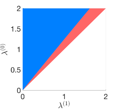
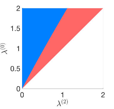
We aim to compare the detection performance of case 0 with cases 1 and 2, respectively. We are interested in identifying the ranges of the detection parameters for which one case performs better than the other. As mentioned previously, the parameters $q^{(k)}$ are fixed for the three cases, so we compare the performance for different values of the parameter $\lambda^{(k)}$ . Fig. 4 presents the performance comparison of case 0 with case 1 (Fig. 4) and case 2 (Fig. 4). Any point $(x,y)$ in the colored regions are achievable by an attack, i.e., there exists an attack $a$ such that $a^{\mathsf{T}}\Lambda^{(k)}a=x$ and $a^{\mathsf{T}}\Lambda^{(0)}a=y$ , whereas the white region is inadmissible (see (34)). The blue region corresponds to the pairs $(\lambda^{(k)},\lambda^{(0)})$ for which case 0 performs better than case $k$ , i.e., $P_{D}(q^{(0)},\lambda^{(0)},P_{F})\geq P_{D}(q^{(k)},\lambda^{(k)},P_{F})$ for $k=1,2$ . In the red region, case $k$ performs better that case 0, $k=1,2$ .

We observe that case 0 performs better than case $k$ if $\frac{\lambda^{(0)}}{\lambda^{(k)}}$ is large, and vice versa. This shows that if the attack vector $a$ is such that $\frac{\lambda^{(0)}}{\lambda^{(k)}}$ is small, then the detection performance corresponding to a more private mechanism ( $\mathcal{M}^{(k)}>\mathcal{M}^{(0)}$ ) is better. This implies that there is non-strict trade-off between privacy and detection performance. This counter-intuitive result is due to the suboptimality of the GLRT used to perform detection, as explained before (c.f. discussion above Remark 3). Further, we observe that the red region of Fig. 4 is larger than (and contains) the red region of Fig. 4. This is because $\mathcal{M}^{(2)}$ is more private than $\mathcal{M}^{(1)}$ .

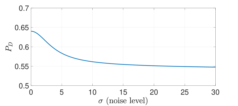
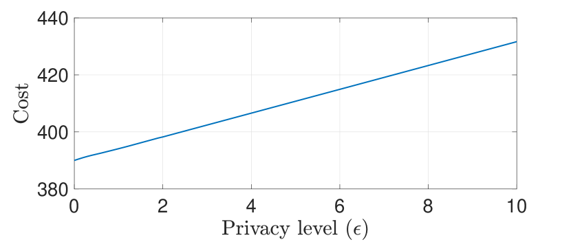
Next, we consider the case where Subsystems $2$ and $3$ implement their privacy mechanisms by only adding artificial noise in (2). Thus, $S_{2}=I_{8},S_{3}=I_{6}$ , and the artificial noise covariances are given by $\Sigma_{\tilde{r}_{2}}=\sigma^{2}I_{8}$ and $\Sigma_{\tilde{r}_{3}}=\sigma^{2}I_{6}$ . The attack on Subsystem $1$ (that is, on generator $1$ ) is $\tilde{a}(k)=2500$ for $k=0,1,2$ . Clearly, as the noise level $\sigma$ increases, the privacy level also increases. Fig. 5 shows the detection performance of Subsystem $1$ for varying noise level $\sigma$ . We observe that the detection performance is a decreasing function of the noise level (c.f. Corollary 5.3), implying a strict trade-off between detection performance and privacy in this case. Finally, we illustrate this strict trade-off by also explicitly solving the optimization problem (40) and computing the optimal noise covariance matrices. We fix the same desired privacy level for Subsystems 2 and 3: $\epsilon_{1}=\epsilon_{2}=\epsilon$ . Fig. 6 shows that the optimal cost in (40) increases with $\epsilon$ , indicating that the detection performance decreases as privacy level increases.

7 Conclusion

We study an attack detection problem in interconnected dynamical systems where each subsystem is tasked with detection of local attacks without any knowledge of the dynamics of other subsystems and their interconnection signals. The subsystems share measurements among themselves to aid attack detection, but they also limit the amount and quality of the shared measurements due to privacy concerns. We show that there exists a non-strict trade-off between privacy and detection performance, and in some cases, sharing less measurements can improve the detection performance. We reason that this counter-intuitive result is due the suboptimality of the considered $\chi^{2}$ test.

Future work includes exploring if this counter-intuitive trade-off exist for alternative detection schemes (for instance, unknown-input observers) and for other types of statistical tests. Also, recursive schemes to compute the state estimates, eliminate interconnections and compute the detection probability will be explored. Finally, privacy ordering of two mechanisms irrespective of their subspaces of shared measurement will be defined using suitable weighing matrix for each subspace.

APPENDIX

Lemma A.1

The optimal solutions of the following weighted least squares problem:

\displaystyle\underset{x}{\min}\quad J(x)=(y-Hx)^{\mathsf{T}}\Sigma^{-1}(y-Hx),

(44)

with $\Sigma>0$ are given by

\displaystyle x^{*}=\tilde{H}^{+}H^{\mathsf{T}}\Sigma^{-1}y+(I-\tilde{H}^{+}\tilde{H})d,

(45)

where $\tilde{H}=H^{\mathsf{T}}\Sigma^{-1}H,$ and $d$ is any real vector of appropriate dimension. Further, the optimal value of the cost is

\displaystyle J(x^{*})=y^{\mathsf{T}}(\Sigma^{-1}-\Sigma^{-1}H\tilde{H}^{+}H^{\mathsf{T}}\Sigma^{-1})y.

(46)

Lemma A.2

Let $\left[\begin{smallmatrix}A&B\\ B^{\mathsf{T}}&D\end{smallmatrix}\right]$ be a positive definite matrix with $A>0$ , $D\geq 0$ . Further, let $M\geq 0$ . Then,

\displaystyle\left[\begin{smallmatrix}A&B\\ B^{\mathsf{T}}&D\end{smallmatrix}\right]^{-1}\geq\left[\begin{smallmatrix}(A+M)^{-1}&0\\ 0&0\end{smallmatrix}\right],

Proof: Using the Schur complement, we have

\displaystyle\left[\begin{smallmatrix}A&B\\ B^{\mathsf{T}}&D\end{smallmatrix}\right]^{-1}=\left[\begin{smallmatrix}I&-A^{-1}B\\ 0&I\end{smallmatrix}\right]\left[\begin{smallmatrix}A^{-1}&0\\ 0&(D-B^{\mathsf{T}}A^{-1}B)^{-1}\end{smallmatrix}\right]\left[\begin{smallmatrix}I&0\\ -B^{\mathsf{T}}A^{-1}&I\end{smallmatrix}\right],

where the Schur complement $D-B^{\mathsf{T}}A^{-1}B>0$ . Further,

\displaystyle\left[\begin{smallmatrix}(A+M)^{-1}&0\\ 0&0\end{smallmatrix}\right]=\left[\begin{smallmatrix}I&-A^{-1}B\\ 0&I\end{smallmatrix}\right]\left[\begin{smallmatrix}(A+M)^{-1}&0\\ 0&0\end{smallmatrix}\right]\left[\begin{smallmatrix}I&0\\ -B^{\mathsf{T}}A^{-1}&I\end{smallmatrix}\right]

Since $A+M\geq A$ , $A^{-1}\geq(A+M)^{-1}$ . Thus,

\displaystyle\left[\begin{smallmatrix}A^{-1}-(A+M)^{-1}&0\\ 0&(D-B^{\mathsf{T}}A^{-1}B)^{-1}\end{smallmatrix}\right]\geq 0,

and the result follows.

Lemma A.3

Let $\Sigma>0\in\mathbb{R}^{n\times n}$ and $\Sigma_{a}\geq 0\in\mathbb{R}^{m\times m},$ with $m\leq n$ , and let $S\in\mathbb{R}^{n\times m}$ be full (column) rank. Then,

\displaystyle\Sigma^{-1}\geq S(S^{\mathsf{T}}\Sigma S+\Sigma_{a})^{-1}S^{\mathsf{T}}.

(47)

Proof: Since $S$ is full column rank, $S^{\mathsf{T}}\Sigma S>0$ , $S^{\mathsf{T}}\Sigma S+\Sigma_{a}$ is invertible and $S^{+}S=I_{m}=S^{\mathsf{T}}(S^{\mathsf{T}})^{+}$ . Thus, $I_{n}=\left[\begin{smallmatrix}S^{\mathsf{T}}(S^{\mathsf{T}})^{+}&0\\ 0&I_{n-m}\end{smallmatrix}\right]$ . Let $N\in\mathbb{R}^{n\times(n-m)}$ denote a matrix whose columns are the basis of $\text{Null}(S^{\mathsf{T}})$ . Then, $\left[\begin{smallmatrix}S^{\mathsf{T}}(S^{\mathsf{T}})^{+}&0\end{smallmatrix}\right]=S^{\mathsf{T}}\left[\begin{smallmatrix}(S^{\mathsf{T}})^{+}&N\end{smallmatrix}\right]\triangleq S^{\mathsf{T}}R.$ Since, $\text{Im}((S^{\mathsf{T}})^{+})=\text{Im}(S)\perp\text{Null}(S^{\mathsf{T}})$ , $R$ is non-singular. Let $T\triangleq\left[\begin{smallmatrix}0&I_{n-m}\end{smallmatrix}\right]R^{-1}$ . Then, we have $I_{n}=\left[\begin{smallmatrix}S^{\mathsf{T}}\\ T\end{smallmatrix}\right]R=R\left[\begin{smallmatrix}S^{\mathsf{T}}\\ T\end{smallmatrix}\right]$ . Thus,

	$\displaystyle\Sigma^{-1}$	$\displaystyle=I_{n}^{\mathsf{T}}(I_{n}\Sigma I_{n}^{\mathsf{T}})^{-1}I_{n}$
		$\displaystyle=\left[\begin{smallmatrix}S&T^{\mathsf{T}}\end{smallmatrix}\right]R^{\mathsf{T}}\left(R\left[\begin{smallmatrix}S^{\mathsf{T}}\\ T\end{smallmatrix}\right]\Sigma\left[\begin{smallmatrix}S&T^{\mathsf{T}}\end{smallmatrix}\right]R^{\mathsf{T}}\right)^{-1}R\left[\begin{smallmatrix}S^{\mathsf{T}}\\ T\end{smallmatrix}\right]$
		$\displaystyle=\left[\begin{smallmatrix}S&T^{\mathsf{T}}\end{smallmatrix}\right]\left(\left[\begin{smallmatrix}S^{\mathsf{T}}\\ T\end{smallmatrix}\right]\Sigma\left[\begin{smallmatrix}S&T^{\mathsf{T}}\end{smallmatrix}\right]\right)^{-1}\left[\begin{smallmatrix}S^{\mathsf{T}}\\ T\end{smallmatrix}\right]$
		$\displaystyle=\left[\begin{smallmatrix}S&T^{\mathsf{T}}\end{smallmatrix}\right]\left[\begin{smallmatrix}S^{\mathsf{T}}\Sigma S&S^{\mathsf{T}}\Sigma T^{\mathsf{T}}\\ T\Sigma S&T\Sigma T^{\mathsf{T}}\end{smallmatrix}\right]^{-1}\left[\begin{smallmatrix}S^{\mathsf{T}}\\ T\end{smallmatrix}\right],\quad\text{and}$
	$\displaystyle S(S^{\mathsf{T}}\Sigma S$	$\displaystyle+\Sigma_{a})^{-1}S^{\mathsf{T}}=\left[\begin{smallmatrix}S&T^{\mathsf{T}}\end{smallmatrix}\right]\left[\begin{smallmatrix}(S^{\mathsf{T}}\Sigma S+\Sigma_{a})^{-1}&0\\ 0&0\end{smallmatrix}\right]^{-1}\left[\begin{smallmatrix}S^{\mathsf{T}}\\ T\end{smallmatrix}\right].$

The result follows from Lemma A.2.

Lemma A.4

Let $M_{1}\geq M_{2}\geq 0$ , $\lambda\geq 0$ and let $J(x)=x^{\mathsf{T}}M_{1}x$ . Then, the maximum and minimum values of $J(x)$ subject to $x^{\mathsf{T}}M_{2}x=\lambda$ are given by $\lambda\mu_{max}$ and $\lambda\mu_{min}$ respectively, where $\mu_{max}$ and $\mu_{min}$ are the largest and smallest generalized eigenvalues of $(M_{1},M_{2})$ , respectively.

Proof: Consider the following optimization problem

\displaystyle\underset{x}{\min/\max}\quad J(x)=x^{\mathsf{T}}M_{1}x,\quad\text{subject to}\quad x^{\mathsf{T}}M_{2}x=\lambda.

The Lagrangian of this problem is given by $l=x^{\mathsf{T}}M_{1}x-\mu(x^{\mathsf{T}}M_{2}x-\lambda)$ , where $\mu\in\mathbb{R}$ is the Lagrange multiplier. By differentiating $l$ , the first order optimality condition is given by $(M_{1}-\mu M_{2})x=0$ . Thus, $\mu$ is a generalized eigenvalue of $(M_{1},M_{2})$ . Further, using $M_{1}x=\mu M_{2}x$ , the cost at the optimum is given by $\lambda\mu$ and the maximum and minimum values of the cost given in the lemma follow.

Lemma A.5

Let $\tilde{H}=H^{\mathsf{T}}\Sigma^{-1}H$ where $\Sigma>0$ and $H$ has a full row rank. Then, $\tilde{H}^{+}=H^{+}\Sigma(H^{+})^{\mathsf{T}}$ .

Proof: Let $\Sigma=RR^{\mathsf{T}}$ be the Cholesky decomposition.

	$\displaystyle\tilde{H}^{+}$	$\displaystyle=((R^{-1}H)^{\mathsf{T}}R^{-1}H)^{+}=(R^{-1}H)^{+}((R^{-1}H)^{+})^{\mathsf{T}}$
		$\displaystyle\overset{(a)}{=}H^{+}RR^{\mathsf{T}}(H^{+})^{\mathsf{T}}=H^{+}\Sigma(H^{+})^{\mathsf{T}},$

where $(a)$ follows since $H$ is full row rank.

References

[1] S. M. Rinaldi, J. P. Peerenboom, and T. K. Kelly. Identifying, understanding, and analyzing critical infrastructure interdependencies. IEEE Control Systems Magazine, 21(6):11–25, 2001.
[2] A. Cardenas, S. Amin, and S. Sastry. Secure control: Towards survivable cyber-physical systems. In International Conference on Distributed Computing Systems Workshops, page 495—500, Beijing, China, 2008.
[3] J. Giraldo, E. Sarkar, A. Cardenas, M. Maniatakos, and M. Kantarcioglu. Security and privacy in cyber-physical systems: A survey of surveys. IEEE Design & Test, 34(4):7–17, 2017.
[4] H. Fawzi, P. Tabuada, and S. Diggavi. Secure estimation and control for cyber-physical systems under adversarial attacks. IEEE Transactions on Automatic Control, 59(6):1454–1467, 2014.
[5] F. Pasqualetti, F. Dörfler, and F. Bullo. Attack detection and identification in cyber-physical systems. IEEE Transactions on Automatic Control, 58(11):2715–2729, 2013.
[6] Y. Chen, S. Kar, and J. M. F. Moura. Dynamic attack detection in cyber-physical systems with side initial state information. IEEE Transactions on Automatic Control, 62(9):4618–4624, 2017.
[7] Y. Mo and B. Sinopoli. On the performance degradation of cyber-physical systems under stealthy integrity attacks. IEEE Transactions on Automatic Control, 61(9):2618–2624, 2016.
[8] Y. Chen, S. Kar, and J. M. F. Moura. Optimal attack strategies subject to detection constraints against cyber-physical systems. IEEE Transactions on Control of Network Systems, 5(3):1157–1168, 2018.
[9] H. Nishino and H. Ishii. Distributed detection of cyber attacks and faults for power systems. In IFAC World Congress, pages 11932–11937, Cape Town, South Africa, August 2014.
[10] S. Cui, Z. Han, S. Kar, T. T. Kim, H. V. Poor, and A. Tajer. Coordinated data-injection attack and detection in the smart grid: A detailed look at enriching detection solutions. IEEE Signal Processing Magazine, 29(5):106–115, 2012.
[11] F. Dörfler, F. Pasqualetti, and F. Bullo. Distributed detection of cyber-physical attacks in power networks: A waveform relaxation approach. In Allerton Conf. on Communications, Control and Computing, September 2011.
[12] F. Pasqualetti, F. Dörfler, and F. Bullo. A divide-and-conquer approach to distributed attack identification. In IEEE Conf. on Decision and Control, pages 5801–5807, Osaka, Japan, December 2015.
[13] N. Forti, G. Battistelli, L. Chisci, S. Li, B. Wang, and B. Sinopoli. Distributed joint attack detection and secure state estimation. IEEE Transactions on Signal and Information Processing over Networks, 4(1):96–110, 2018.
[14] Y. Guan and X. Ge. Distributed attack detection and secure estimation of networked cyber-physical systems against false data injection attacks and jamming attacks. IEEE Transactions on Signal and Information Processing over Networks, 4(1):48–59, 2018.
[15] F. Boem, A. J. Gallo, G. Ferrari-Trecate, and T. Parisini. A distributed attack detection method for multi-agent systems governed by consensus-based control. In IEEE Conf. on Decision and Control, pages 5961–5966, Melbourne, Australia, 2017.
[16] A. Teixeira, H. Sandberg, and K. H. Johansson. Networked control systems under cyber attacks with applications to power networks. In American Control Conference, pages 3690–3696, 2010.
[17] R. Anguluri, V. Katewa, and F. Pasqualetti. Centralized versus decentralized detection of attacks in stochastic interconnected systems. IEEE Transactions on Automatic Control, 2019. To appear.
[18] R. M. G. Ferrari, T. Parisian, and M. M. Polycarpou. Distributed fault detection and isolation of large-scale discrete-time nonlinear systems: An adaptive approximation approach. IEEE Transactions on Automatic Control, 57(2):275–290, 2012.
[19] C. Kiliris, M. M. Polycarpou, and T. Parisian. A robust nonlinear observer-based approach for distributed fault detection of input–output interconnected systems. Automatica, 53:408–415, 2015.
[20] V. Reppa, M. M. Polycarpou, and C. G. Panayiotou. Distributed sensor fault diagnosis for a network of interconnected cyber-physical systems. IEEE Transactions on Control of Network Systems, 2(1):11–23, 2015.
[21] X. Zhang and Q. Zhang. Distributed fault diagnosis in a class of interconnected nonlinear uncertain systems. International Journal of Control, 85(11):1644–1662, 2012.
[22] X. G. Yan and C. Edwards. Robust decentralized actuator fault detection and estimation for large-scale systems using a sliding mode observer. International Journal of Control, 81(4):591–606, 2008.
[23] E. Franco, R. Olfati-Saber, T. Parisini, and M. M. Polycarpou. Distributed fault diagnosis using sensor networks and consensus-based filters. In IEEE Conf. on Decision and Control, pages 386–391, San Diego, CA, USA, December 2006.
[24] S. Stankovic, N. Ilic, Z. Djurovic, M. Stankovic, and K. H. Johansson. Consensus based overlapping decentralized fault detection and isolation. In Conference on Control and Fault Tolerant Systems, Nice, France, 2010.
[25] I. Shames, A. M. H. Teixeira, H. Sandberg, and K. H. Johansson. Distributed fault detection for interconnected second-order systems. Automatica, 47:2757–2764, 2011.
[26] J. Cortes, G. E. Dullerud, S. Han, J. Le Ny, S. Mitra, and G. J. Pappas. Differential privacy in control and network systems. In IEEE Conf. on Decision and Control, pages 4252–4272, Las Vegas, USA, 2016.
[27] E. Akyol, C. Langbort, and T. Basar. Privacy constrained information processing. In IEEE Conf. on Decision and Control, Osaka, Japan, 2015.
[28] F. Farokhi and G. Nair. Privacy-constrained communication. In IFAC Workshop on Distributed Estimation and Control in Networked Systems, pages 43–48, Tokyo, Japan, September 2016.
[29] T. Tanaka, M. Skoglund, H. Sandberg, and K. H. Johansson. Directed information and privacy loss in cloud-based control. In American Control Conference, Seattle, USA, 2017.
[30] F. Farokhi and H. Sandberg. Ensuring privacy with constrained additive noise by minimizing fisher information. Automatica, 99:275–288, 2019.
[31] V. Katewa, F. Pasqualetti, and V. Gupta. On privacy vs cooperation in multi-agent systems. International Journal of Control, 91(7):1693–1707, 2018.
[32] Y. Mo and R. M. Murray. Privacy-preserving average consensus. IEEE Transactions on Automatic Control, 62(2):753–765, 2017.
[33] J. Giraldo, A. Cardenas, and M. Kantarcioglu. Security and privacy trade-offs in cps by leveraging inherent differential privacy. In IEEE Conference on Control Technology and Applications, pages 1313–1318, Hawaii, USA, 2017.
[34] R. Anguluri, V. Katewa, and F. Pasqualetti. On the role of information sharing in the security of interconnected systems. In Asia-Pacific Signal and Information Processing Association Annual Summit and Conference, Honolulu, Hi, 2018.
[35] A. S. Willsky. A survey of design methods for failure detection in dynamic systems. Automatica, 12:601–611, 1976.
[36] L. Wasserman. All of Statistics: A Concise Course in Statistical Inference. Springer, 2004.
[37] N. L. Johnson, S. Kotz, and N. Balakrishnan. Continuous Univariate Distributions, Volume 2. Wiley-Interscience, 1995.
[38] E. Furman and R. Zitikis. A monotonicity property of the composition of regularized and inverted-regularized gamma functions with applications. Journal of Mathematical Analysis and Applications, 348(2):971–976, 2008.
[39] E. L. Lehmann and J. P. Romano. Testing Statistical Hypotheses. Springer-Verlag New York, 2005.
[40] R. E. Hartwig. A note on the partial ordering of positive semi-definite matrices. Linear and Multilinear Algebra, 6(3):223–226, 1978.
[41] L. Vandenberghe and S. Boyd. Semidefinite programming. SIAM Review, 38(1):49–95, 1996.
[42] T. Athay, R. Podmore, and S. Virmani. A practical method for the direct analysis of transient stability. IEEE Transactions on Power Apparatus and Systems, PAS-98(2):573–584, 1979.
[43] P. Kundur. Power System Stability and Control. McGraw-Hill Education, 1994.

	$\displaystyle\frac{f(z\|H_{0})}{\underset{a}{\sup}f(z\|H_{1})}\overset{H_{0}}{\underset{H_{1}}{\gtrless}}\tau^{\prime}\quad\text{where,}$	(19)
$\displaystyle f(z\|H_{0})$	$\displaystyle=\frac{1}{\sqrt{2\pi\|\Sigma_{v_{P}}\|}}e^{-\frac{1}{2}z^{\mathsf{T}}\Sigma_{v_{P}}^{-1}z}\quad\text{and,}$
$\displaystyle f(z\|H_{1})$	$\displaystyle=\frac{1}{\sqrt{2\pi\|\Sigma_{v_{P}}\|}}e^{-\frac{1}{2}(z-M^{\mathsf{T}}F_{a}a)^{\mathsf{T}}\Sigma_{v_{P}}^{-1}(z-M^{\mathsf{T}}F_{a}a)},$