On a spectral method for $\beta$ -particle bound excitation collisions in kilonovae

Ryan T. Wollaeger Center for Theoretical Astrophysics, Los Alamos National Laboratory, Los Alamos, NM 87545, USA Computer, Computational, and Statistical Sciences Division, Los Alamos National Laboratory, Los Alamos, NM 87545, USA Chris L. Fryer Center for Nonlinear Studies, Los Alamos National Laboratory, Los Alamos, NM 87545, USA Center for Theoretical Astrophysics, Los Alamos National Laboratory, Los Alamos, NM 87545, USA The University of Arizona, Tucson, AZ 85721, USA Department of Physics and Astronomy, The University of New Mexico, Albuquerque, NM 87131, USA The George Washington University, Washington, DC 20052, USA Robert Chiodi Computer, Computational, and Statistical Sciences Division, Los Alamos National Laboratory, Los Alamos, NM 87545, USA Peter T. Brady Computer, Computational, and Statistical Sciences Division, Los Alamos National Laboratory, Los Alamos, NM 87545, USA Oleg Korobkin Center for Theoretical Astrophysics, Los Alamos National Laboratory, Los Alamos, NM 87545, USA T-5 Applied Mathematics and Plasma Physics Group, Los Alamos National Laboratory, Los Alamos, NM 87545, USA Cale Harnish Computer, Computational, and Statistical Sciences Division, Los Alamos National Laboratory, Los Alamos, NM 87545, USA Christopher J. Fontes Center for Theoretical Astrophysics, Los Alamos National Laboratory, Los Alamos, NM 87545, USA Computational Physics Division, Los Alamos National Laboratory, Los Alamos, NM, 87545, USA Jeffrey R. Haack Computer, Computational, and Statistical Sciences Division, Los Alamos National Laboratory, Los Alamos, NM 87545, USA Oleksandr Chapurin T-5 Applied Mathematics and Plasma Physics Group, Los Alamos National Laboratory, Los Alamos, NM 87545, USA Oleksandr Koshkarov T-5 Applied Mathematics and Plasma Physics Group, Los Alamos National Laboratory, Los Alamos, NM 87545, USA Gian Luca Delzanno T-5 Applied Mathematics and Plasma Physics Group, Los Alamos National Laboratory, Los Alamos, NM 87545, USA Daniel Livescu Computer, Computational, and Statistical Sciences Division, Los Alamos National Laboratory, Los Alamos, NM 87545, USA

Abstract

The interaction of $\beta$ -particles with the weakly ionized plasma background is an important mechanism for powering the kilonova transient signal from neutron star mergers. For this purpose, we present an implementation of the approximate fast-particle collision kernel, described by Inokuti (1971) following the seminal formulation of Bethe (1930), in a spectral solver of the Vlasov-Maxwell-Boltzmann equations. In particular, we expand the fast-particle plane-wave atomic excitation kernel into coefficients of the Hermite basis, and derive the relevant discrete spectral system. In this fast-particle limit, the approach permits the direct use of atomic data, including optical oscillator strengths, normally applied to photon-matter interaction. The resulting spectral matrix is implemented in the MASS-APP spectral solver framework, in a way that avoids full matrix storage per spatial zone. We numerically verify aspects of the matrix construction, and present a proof-of-principle 3D simulation of a 2D axisymmetric kilonova ejecta snapshot. Our preliminary numerical results indicate that a reasonable choice of Hermite basis parameters for $\beta$ -particles in the kilonova are a bulk velocity parameter $\vec{u}=0$ , a thermal velocity parameter $\vec{\alpha}=0.5c$ , and a 9x9x9 mode velocity basis set (Hermite orders 0 to 8 in each dimension). For ejecta-interior sample zones, we estimate the ratio of thermalization from large-angle ( $\gtrsim 2.5^{\circ}$ ) bound excitation scattering to total thermalization is $\sim$ 0.002-0.003.

methods: numerical — plasmas — stars: neutron

^†^†software: FleCSI (Bergen et al., 2016), Kokkos (Trott et al., 2021), MASS-APP

1 Introduction

Kilonovae (KNe) are radioactively powered electromagnetic (EM) transients signaling the aftermath of double neutron star or neutron star-black hole binary mergers (an incomplete sequence of KN model developments up to 2017 might be given by Lattimer & Schramm (1974, 1976); Li & Paczyński (1998); Freiburghaus et al. (1999); Roberts et al. (2011); Kasen et al. (2013); Tanaka & Hotokezaka (2013); Fontes et al. (2015a); Barnes et al. (2016); Metzger (2017)). As the two compact objects inspiral due to the emission of gravitational waves, the neutron star(s) will be tidally disrupted, causing neutron-rich mass to eject and become gravitationally unbound. The merger results in a compact remnant (neutron star or black hole) surrounded by an accretion disk, from which various mechanisms produce further (“post-merger”) ejecta (see, for example, Perego et al. (2014); Martin et al. (2015); Desai et al. (2022)). The detailed EM spectra and broadband magnitudes from the observation of KN AT2017gfo (see, for example, Arcavi et al. (2017); Cowperthwaite et al. (2017); Drout et al. (2017); Kasliwal et al. (2017); Smartt et al. (2017); Tanvir et al. (2017); Troja et al. (2017); Villar et al. (2017)), in concert with the gravitational wave observation GW170817 (Abbott et al., 2017a, b), provided an unprecedented window into the pre- and post-merger phases of the transient, and by examining the nuclear decay pattern in the ejecta seemed to confirm neutron star mergers are a source of r-process elements (Rosswog et al., 2018).

While the basic picture of KNe has remained unchanged for several decades, since the semi-analytic work of Li & Paczyński (1998) (for a review of KN physics, see also Metzger (2019)), simulating KNe at high fidelity is an ever-developing field. Recent studies explore detailed radiative transfer, atomic physics, non-local thermodynamic equilibrium (non-LTE), and multidimensional spatial ejecta, for instance: Fontes et al. (2020); Tanaka et al. (2020); Fontes et al. (2023) on detailed LTE opacity, Hotokezaka et al. (2021); Pognan et al. (2022a, b, 2023) on detailed non-LTE opacity, and Korobkin et al. (2021); Heinzel et al. (2021); Bulla (2023); Fryer et al. (2023) on spatial distribution and multidimensional spatial effects (and see references therein). Each of these aspects brings a level of uncertainty into the simulations, that otherwise might be encapsulated in free parameters (for example, grey opacity). A large source of uncertainty in state-of-the-art calculations, particularly at late times as the KN ejecta becomes nebular, is in modeling the interaction of decay products ( $\alpha$ , $\beta$ , and $\gamma$ particles) with the ions forming the ejecta. In full generality, it is a complicated problem of multiple particle fields undergoing transfer and interaction with atomic orbital structure and free electrons. Moreover, the atomic structure of the elements formed in r-process can involve tens of millions of resonances between thousands to millions of energy levels (see, for example, the atomic data presented by Fontes et al. (2020); Tanaka et al. (2020)).

The process of $\beta$ -particle thermalization (the loss of particle kinetic energy to Coulomb interactions, atomic excitations, ionizations, etc.) is inefficient compared to thermalization of the more massive $\alpha$ particles or fission fragments (Barnes et al., 2016, 2021; Zhu et al., 2021), and hence is non-local ( $\beta$ -particles travel significant length scales relative to the ejecta to deposit energy). Barnes et al. (2016, 2021) and Zhu et al. (2021) have demonstrated this inefficiency significantly impacts the observable EM KN signal (on the order of a factor of 2 in luminosity, for instance). The state-of-the-art detailed thermalization model for $\beta$ -particles presented by Barnes et al. (2021) uses the Bethe stopping-potential prescription (Bethe, 1930), which accounts for energy loss over a particle path due to multiple small-angle scatters and encapsulates atomic properties with an average ionization. A question remains as to the impact of large-angle scatters that induce excitation effects in the ion background, which in principle requires the so-called “generalized” oscillator strengths that were introduced by Bethe (1930) and elaborated on by Inokuti (1971).

Consequently, having a framework for implementing atomic data directly into a thermalization calculation, along with a formulation for particle transfer that can be extended to different differential cross sections, is useful for making inroads to improved fidelity. We attempt one such preliminary inroad using a deterministic spectral plasma solver implemented in the CPU/GPU-parallel Multiphysics Adaptive Scalable Simulator for Applications in Plasma Physics (MASS-APP) code base (Chiodi & Brady, P. T. et al., in prep.). “Spectral” in this context implies the particle phase space distribution function is expanded over a complete basis function set in velocity space. To undertake proof-of-concept simulations, we implement the non-relativistic inelastic scattering kernel for excitation, described by Inokuti (1971). The inelastic form of the two-body, or binary, integral collision kernel is given by Garibotti & Spiga (1994), and has been used before in the context of spectral Boltzmann methods (see, for instance the spectral-Lagrangian Boltzmann equation solver by Munafò et al. (2014)). Here we specifically employ an asymmetrically weighted Hermite function basis (Armstrong et al., 1970), which has a beneficial property of bridging macro (fluid)-micro (kinetic) scales (see, for example, Camporeale et al. (2006); Vencels et al. (2015); Delzanno (2015); Koshkarov et al. (2021)). The derivational sequence we present here is similar to the Hermite expansion of the multi-species collision kernel presented by Wang & Cai (2019); Li et al. (2022, 2023), but we do not expand both distributions into the binary kernel, instead expanding one and also expanding the cross section itself in the Hermite basis. We also make approximations to the kernel that make the integral over the ion species separable from the integral over $\beta$ -particle velocity (which generally will not hold outside the fast-particle approximation). This permits us to employ an efficient closed form for integrals of products involving three Hermite polynomials and two Gaussian weights, which to our knowledge is not used by Wang & Cai (2019); Li et al. (2022, 2023), since their kernel expansion does not isolate these terms (to be sure, the approaches of these authors are more general, in being able to solve for multiple distribution species).

Neglecting internal conversion, $\beta$ -particle emission has a smooth continuum (Fermi, 1934; Schenter & Vogel, 1983; Alekseev et al., 2020) for a spectrum, lending itself well to smooth basis functions. Hence, we see this spectral Hermite basis technique as a possible deterministic supplement to Particle-in-Cell (PIC) or Monte Carlo methods that may be better suited to treating sharp electron emission lines resulting from internal conversion. Moreover, deterministic schemes of course do not have stochastic noise, so they may be well suited to capturing large-angle scattering effects, specifically.

This paper is organized as follows. In Section 2, we write the governing equations solved with MASS-APP and describe the derivation of the excitation collision kernel used for $\beta$ -particles. In Section 3, we present numerical verification of particular aspects of the method, comparing closed form derivations to direct numerical integration of terms that build the collision matrix needed for simulation. In Section 4, we describe a trial $\beta$ -particle simulation of excitation interactions for a 2D axisymmetric morphology embedded in 3D Cartesian geometry. Finally, in Section 5 we summarize our findings and discuss future work that would further improve fidelity.

2 Spectral Method and Implementation

In this section, we write down the full spectrally discretized set of equations. Subsequently, we focus attention on incorporating the non-relativistic differential excitation cross section given by Inokuti (1971) into the spectral basis framework, and discuss the approximations made to simplify the collision kernel. After deriving the spectral Hermite form of the fast-particle kernel, we provide an outline summarizing the calculations of this section, including how the steps may be extensible to other differential cross sections. Supplementary detail is provided in Appendix A for the evaluation of the two-body collision kernel and in Appendix B for the closed-form evaluation of integrals involving three Hermite polynomials and two Gaussian weight functions, referred to henceforth as “compact triple Hermite products”, which are used to evaluate each term in the spectrally discrete collision matrix derived in this section.

The Vlasov-Maxwell-Boltzmann system of equations we consider is


	$\displaystyle\frac{\partial f_{s}}{\partial t}+\vec{v}\cdot\nabla f_{s}+\frac{q_{s}}{m_{s}}(\vec{E}+\vec{v}\times\vec{B})\cdot\nabla_{v}f_{s}=\mathcal{C}[f_{a},f_{s}]\;\;,$		(1a)
	$\displaystyle\frac{\partial\vec{E}}{\partial t}=c\nabla\times\vec{B}-4\pi\vec{J}\;\;,$		(1b)
	$\displaystyle\frac{\partial\vec{B}}{\partial t}=-c\nabla\times\vec{E}\;\;,$		(1c)
	$\displaystyle\vec{J}=q_{s}\int\vec{v}f_{s}d^{3}\vec{v}+q_{a}\int\vec{v}f_{a}d^{3}\vec{v}\;\;,$		(1d)

where $t$ is time, $\vec{v}$ is velocity, the $\nabla$ operator is the gradient with respect to the spatial coordinate ( $\vec{x}$ ), $\nabla_{v}$ is the gradient operator with respect to velocity, subscript $s$ indicates the species ( $\beta$ -particles here), subscript $a$ indicates the atom/ion background, $q_{s}$ is charge, $m_{s}$ is mass, $\vec{E}$ and $\vec{B}$ are the electric and magnetic fields, $f_{s}$ and $f_{a}$ are the $\beta$ -particle and background distributions (number density per spatial volume per velocity volume), $\vec{J}$ is the current density, and $\mathcal{C}[\cdot,\cdot]$ is the collision operator. For the purpose of this work, we set the interacting distribution of ejecta atom/ions as given within a discrete time step, thus linearizing the collision term. This approach is consistent with the practice of computing decay thermalization and radiative transfer in separate steps from the ejecta plasma state update, but may incur error where moderate bulk thermodynamic changes lead to significant electron occupation number discrepancy for particular atomic states.

The Hermite basis is orthogonal with respect to a Gaussian weight, hence amenable to determining expansion coefficients via inner products. Following Delzanno (2015), we expand the distribution as

f_{s}(\vec{x},\vec{v},t)=\sum_{n,m,p}C_{n,m,p}(\vec{x},t)\Psi_{n,m,p}(\vec{\xi})\;\;,

(2)

where the subscripts $n$ , $m$ , and $p$ are the order of the basis function in each velocity dimension, $C_{n,m,p}$ is the expansion coefficient (for which we solve), and the basis function $\Psi_{n,m,p}(\vec{\xi})$ is given by Eq. (B3). The $\vec{\xi}$ argument of the basis functions is non-dimensional velocity (subscript $xyz$ indicates component),

\vec{\xi}=(\xi_{x},\xi_{y},\xi_{z})=\left(\frac{v_{x}-u_{x}}{\alpha_{x}},\frac{v_{y}-u_{y}}{\alpha_{y}},\frac{v_{z}-u_{z}}{\alpha_{z}}\right)=(\vec{v}-\vec{u})\oslash\vec{\alpha}\;\;,

(3)

where $\vec{u}$ and $\vec{\alpha}$ are user-provided, constant velocity parameters corresponding to bulk and thermal velocity in the Gaussian factor of the basis. The last equality represents $\vec{\xi}$ with Hadamard (element-wise) division.

The system of equations resulting from expanding Eqs. (1) with Eq. (2) and taking Hermite inner products is (see, for example, Delzanno (2015))


	$\displaystyle\frac{\partial C_{n,m,p}}{\partial t}+\;{\ldots}\;=\sum_{n^{\prime},m^{\prime},p^{\prime}}S_{n,m,p}^{n^{\prime},m^{\prime},p^{\prime}}C_{n^{\prime},m^{\prime},p^{\prime}}\;\;,$		(4a)
	$\displaystyle\frac{\partial\vec{B}}{\partial t}=-c\nabla\times\vec{E}\;\;,$		(4b)
	$\displaystyle\frac{\partial\vec{E}}{\partial t}=c\nabla\times\vec{B}-4\pi q_{s}\alpha_{x}\alpha_{y}\alpha_{z}\left(C_{0,0,0}\begin{bmatrix}u_{x}\\ u_{y}\\ u_{z}\end{bmatrix}+\frac{1}{\sqrt{2}}\begin{bmatrix}\alpha_{x}C_{1,0,0}\\ \alpha_{y}C_{0,1,0}\\ \alpha_{z}C_{0,0,1}\end{bmatrix}\right)\;\;,$		(4c)

where $S_{n,m,p}^{n^{\prime},m^{\prime},p^{\prime}}$ is a collision matrix dependent on the background ion properties of the KN ejecta, and in Eq. (4)c we have made the approximation that the ion background does not contribute significant current density. For brevity, on the left side of Eq. (4)a, we have omitted a spatial divergence operator including the flux and Lorentz force from $\vec{E}$ and $\vec{B}$ , but include them in a version of the equations in Appendix C.

2.1 Fast-particle, non-relativistic, differential cross section

We derive the non-relativistic form of the scattering matrix $S_{n,m,p}^{n^{\prime},m^{\prime},p^{\prime}}$ using the differential cross section in the Bethe-Born (high-energy) limit, presented by Inokuti (1971) for excitation from atomic state $j^{\prime}$ to atomic state $j$ ,

\frac{d\sigma_{jj^{\prime}}}{d\Omega}=4\left(\frac{Me^{2}}{\hbar^{2}}\right)^{2}\left(\frac{k^{\prime}}{k}\right)K^{-4}\left(\frac{R}{E_{jj^{\prime}}}\right)(Ka_{0})^{2}f_{jj^{\prime}}(K)\;\;,

(5)

where

M=\frac{m_{e}M_{a}}{m_{e}+M_{a}}

(6)

is the reduced mass ( $m_{e}$ and $M_{a}$ are electron and atomic mass), $e$ is the electron charge, $\hbar$ is the reduced Planck constant, $k$ ( $k^{\prime}$ ) is the incoming (outgoing) wave number (equivalently momentum $=\hbar k$ ) of the free electron, $K$ is the magnitude of the difference of the incoming and outgoing wave numbers, $R=m_{e}e^{4}/2\hbar^{2}=13.606$ eV is the Rydberg energy, $E_{jj^{\prime}}$ is the energy difference between levels $j$ and $j^{\prime}$ , $a_{0}=\hbar^{2}/(m_{e}e^{2})=0.52918\times 10^{-8}$ cm is the Bohr radius, and $f_{jj^{\prime}}(K)$ is the generalized oscillator strength. The magnitudes of wave number obey the law of cosines,

K^{2}=k^{2}+(k^{\prime})^{2}-2k^{\prime}k\cos(\theta)\;\;,

(7)

where $\theta$ is the polar angle of deflection in the center-of-mass frame. If the magnitude of pre- and post-deflection wave numbers is taken to be independent of the polar deflection angle, then

\frac{d(K^{2})}{d\theta}=2k^{\prime}k\sin(\theta)\;\;,

(8)

which is given by Inokuti (1971) to replace the solid angle differential $d\Omega$ with $d(K^{2})$ . Assuming $k^{\prime}=k$ , then $K^{2}=2k^{2}(1-\cos(\theta))=4k^{2}\sin^{2}(\theta/2)$ , and Eq. (5) becomes

\frac{d\sigma_{jj^{\prime}}}{d\Omega}=\left(\frac{Me^{2}}{\hbar^{2}}\right)^{2}\frac{\csc^{4}(\theta/2)}{4k^{4}}\left[\left(\frac{R}{E_{jj^{\prime}}}\right)(Ka_{0})^{2}f_{jj^{\prime}}(K)\right]\;\;,

(9)

Supposing an elastic collision, conservation of kinetic energy and momentum imply

k^{\prime}=k\left(\frac{\cos(\theta)+\sqrt{(M_{a}/m_{e})^{2}-\sin^{2}(\theta)}}{1+M_{a}/m_{e}}\right)\;\;,

(10)

where the higher root is taken, so that the solution would be correct if $M_{a}=m_{e}$ . Consequently,

\lim_{M_{a}/m_{e}\rightarrow\infty}k^{\prime}=k\;\;,

(11)

so the condition of $k^{\prime}=k$ , giving Eq. (9) is equivalent to $m_{e}\ll M_{a}$ for elastic collisions. Also in this limit, the reduced mass converges to the electron mass $m_{e}$ , and noting $\hbar k=m_{e}v_{0}$ , where $v_{0}$ is the initial electron velocity, Eq. (9) becomes

\frac{d\sigma_{jj^{\prime}}}{d\Omega}=\left(\frac{e^{2}}{2m_{e}v_{0}^{2}}\right)^{2}\csc^{4}(\theta/2)\left[\left(\frac{R}{E_{jj^{\prime}}}\right)(Ka_{0})^{2}f_{jj^{\prime}}(K)\right]\;\;,

(12)

where the coefficient outside the brackets on the right side is now the standard non-relativistic definition of classical Rutherford scattering (a more general form is noted by Inokuti (1971) as the coefficient, not making the assumption of $m_{e}\ll M_{a}$ ). According to Inokuti (1971), the term in the square brackets is the conditional probability that the atom will excite from state $j^{\prime}$ to state $j$ , given a magnitude of momentum exchange from the electron of $K$ .

It is notable that, $k=k^{\prime}$ does not imply $K$ is small; the angle $\theta$ has to vanish for $K$ to vanish. Using Eq. (7) and conservation of kinetic energy, balanced with excitation, the formula for $(Ka_{0})^{2}$ in terms of initial electron kinetic energy $E_{k}=mv_{0}^{2}/2$ and $\theta$ is (Inokuti, 1971)

(Ka_{0})^{2}=2\frac{E_{k}}{R}\left(\frac{M}{m_{e}}\right)^{2}\left[1-\frac{1}{2}\left(\frac{m_{e}E_{jj^{\prime}}}{ME_{k}}\right)-\left(\sqrt{1-\left(\frac{m_{e}E_{jj^{\prime}}}{ME_{k}}\right)}\right)\cos(\theta)\right]\;\;.

(13)

$(Ka_{0})^{2}$ has the following limits, corresponding to $\theta=0$ or $\pi$ in Eq. (13) (Inokuti, 1971):


	$\displaystyle(Ka_{0})_{\min}^{2}\approx\frac{1}{4}\left(\frac{E_{jj^{\prime}}^{2}}{RE_{k}}\right)\left[1+\frac{1}{2}\left(\frac{m_{e}E_{jj^{\prime}}}{MR}\right)\right]\;\;,$		(14a)
	$\displaystyle(Ka_{0})_{\max}^{2}\approx 4\frac{E_{k}}{R}\left(\frac{M}{m_{e}}\right)^{2}\left[1-\frac{1}{2}\left(\frac{m_{e}E_{jj^{\prime}}}{ME_{k}}\right)\right]\;\;,$		(14b)

where the square root coefficient of $\cos(\theta)$ has been Taylor expanded in $m_{e}E_{jj^{\prime}}/(ME_{k})$ (Inokuti, 1971). The assumption that $E_{k}\gg E_{jj^{\prime}}$ and $E_{k}\gg R$ implies the maximum value of $(Ka_{0})_{\max}^{2}\gg 1$ . However, the Rutherford coefficient of Eq. (12) grows rapidly as $\theta$ vanishes. Moreover, the generalized oscillator strength decreases rapidly for large $Ka_{0}$ (see Inokuti (1971), Section 3.2). Thus, low $Ka_{0}$ and small-angle deflections, i.e. forwarding scattering, are most probable from the Bethe kernel. If the generalized oscillator strength is expanded in a Taylor series as a function of $Ka_{0}$ (Inokuti, 1971), and assuming $(Ka_{0})^{2}\sim(Ka_{0})_{\min}^{2}$ due to the dominance of forward scattering, it becomes reasonable to replace the generalized oscillator strength with the optical oscillator strength, $f_{jj^{\prime}}\approx f_{jj^{\prime}}(K=0)$ , which is the essence of the Bethe high-energy approximation.

If we take $f_{jj^{\prime}}=f_{jj^{\prime}}(K=0)$ , we may readily use the oscillator strength data used for photon opacities in Eq. (12). Doing so, and also incorporating Eq. (13) into Eq. (12), we have a non-relativistic excitation cross section from state $j^{\prime}$ to state $j$ ,

\frac{d\sigma_{jj^{\prime}}}{d\Omega}=2\left(\frac{e^{2}}{4E_{k}}\right)^{2}\csc^{4}(\theta/2)\left(\frac{E_{k}}{E_{jj^{\prime}}}\right)f_{jj^{\prime}}\left[1-\frac{1}{2}\left(\frac{E_{jj^{\prime}}}{E_{k}}\right)-\left(\sqrt{1-\left(\frac{E_{jj^{\prime}}}{E_{k}}\right)}\right)\cos(\theta)\right]\;\;,

(15)

where $m_{e}=M$ has been incorporated into Eq. (13). The only quantity with units on the right side is $(e^{2}/4E_{k})^{2}$ which should have units of length-squared. In electrostatic cgs units (used by Inokuti 1971), so

\left(\frac{e^{2}}{4E_{k}}\right)^{2}\approx\left(\frac{197}{548}\frac{1}{E_{k,{\rm MeV}}}\right)^{2}{\rm fm}^{2}\;\;,

(16)

where $E_{k,{\rm MeV}}$ is the initial kinetic energy in MeV and fm=femtometers.

2.2 Spectral matrix from binary collision kernel

We now incorporate Eq. (15) into the two-body inelastic collision kernel (the elastic version is given by Mihalas & Mihalas (1984), Chapter 1, for example). For our purpose, we decompose the atomic distribution into sub-distributions corresponding to each excited state $j^{\prime}$ , and expand the collision kernel as follows,

\mathcal{C}[f_{a},f_{s}]=\sum_{(j,j^{\prime})\in\mathcal{T}}\mathcal{C}_{jj^{\prime}}[f_{a,j^{\prime}},f_{a,j},f_{s}]\;\;,

(17)

where $\mathcal{T}$ is the set of possible state transition pairs $(j,j^{\prime})$ ,

\mathcal{C}_{jj^{\prime}}[f_{a,j^{\prime}},f_{a,j},f_{s}]=\int\int|\vec{v}_{a}-\vec{v}_{s}|\frac{d\sigma_{jj^{\prime}}}{d\Omega}\left(\frac{g_{j^{\prime}}}{g_{j}}f_{s}(\vec{v}_{s}^{\prime})f_{a,j}(\vec{v}_{a}^{\prime})-f_{s}(\vec{v}_{s})f_{a,j^{\prime}}(\vec{v}_{a})\right)d\Omega d^{3}\vec{v}_{a}\;\;,

(18)

and we have subscripted velocities to indicate ion (“a”) or $\beta$ -particle (“s”). We note this expression follows Munafò et al. (2014), where the energy level degeneracy is included as a coefficient of the product of distributions over post-scattered velocities. The distribution prime superscript indicates evaluation at the post-collision momentum.

Post-scatter velocities $\vec{v}_{a}^{\prime}$ and $\vec{v}_{s}^{\prime}$ can be evaluated from conservation of momentum and energy in the non-relativistic limit, giving


	$\displaystyle\vec{v}_{s}^{\prime}=\frac{1}{m_{e}+M_{a}}\left(m_{e}\vec{v}_{s}+M_{a}\vec{v}_{a}+M_{a}\left(\sqrt{v_{sa}^{2}-\frac{2E_{jj^{\prime}}}{M}}\right)\hat{\Omega}^{\prime}\right)\;\;,$		(19a)
	$\displaystyle\vec{v}_{a}^{\prime}=\frac{1}{m_{e}+M_{a}}\left(m_{e}\vec{v}_{s}+M_{a}\vec{v}_{a}-m_{e}\left(\sqrt{v_{sa}^{2}-\frac{2E_{jj^{\prime}}}{M}}\right)\hat{\Omega}^{\prime}\right)\;\;,$		(19b)

where $v_{sa}=|\vec{v}_{sa}|=|\vec{v}_{a}-\vec{v}_{s}|$ . Equations (19) show the post-scatter velocities as a function of pre-scatter velocity and energy weight, which must be incorporated into Eq. (18) to evaluate the post-scatter portion of the integral (Garibotti & Spiga, 1994).

Considering only excitation collisions in Eq. (1), and expanding the $\beta$ -distribution $f_{s}$ with Eq. (3),

\sum_{n,m,p}\frac{\partial C_{n,m,p}}{\partial t}\Psi_{n,m,p}(\vec{\xi})=\sum_{n,m,p}C_{n,m,p}\int\int v_{sa}\frac{d\sigma_{jj^{\prime}}}{d\Omega}\frac{g_{j^{\prime}}}{g_{j}}\Psi_{n,m,p}(\vec{\xi}^{\prime})f_{a,j}(\vec{v}_{a}^{\prime})d\Omega d^{3}\vec{v}_{a}\\ -\sum_{n,m,p}C_{n,m,p}\int\int v_{sa}\frac{d\sigma_{jj^{\prime}}}{d\Omega}\Psi_{n,m,p}(\vec{\xi})f_{a,j^{\prime}}(\vec{v}_{a})d\Omega d^{3}\vec{v}_{a}\;\;,

(20)

where $\vec{\xi}^{\prime}$ is the non-dimensional form of the post-scatter velocity $\vec{v}_{s}^{\prime}$ . Taking the basis inner product, Eq. (20) becomes

\frac{\partial C_{n^{\prime},m^{\prime},p^{\prime}}}{\partial t}=\sum_{n,m,p}C_{n,m,p}\int\Psi^{n^{\prime},m^{\prime},p^{\prime}}(\vec{\xi})\int\int v_{sa}\frac{d\sigma_{jj^{\prime}}}{d\Omega}\frac{g_{j^{\prime}}}{g_{j}}\Psi_{n,m,p}(\vec{\xi}^{\prime})f_{a,j}(\vec{v}_{a}^{\prime})d\Omega d^{3}\vec{v}_{a}d^{3}\vec{\xi}\\ -\sum_{n,m,p}C_{n,m,p}\int\Psi^{n^{\prime},m^{\prime},p^{\prime}}(\vec{\xi})\int\int v_{sa}\frac{d\sigma_{jj^{\prime}}}{d\Omega}\Psi_{n,m,p}(\vec{\xi})f_{a,j^{\prime}}(\vec{v}_{a})d\Omega d^{3}\vec{v}_{a}d^{3}\vec{\xi}\;\;.

(21)

The right side of Eq. (21) is now in the form of a matrix product with the spectral solution vector $C_{n,m,p}$ , as in the right side of Eq. (4). Following Munafò et al. (2014), the integral in the first summation on the right side of (21) permits us to use the principle of micro-reversibility,

v_{sa}\frac{d\sigma_{jj^{\prime}}}{d\Omega}d\Omega d^{3}\vec{v}_{a}d^{3}\vec{\xi}=\frac{g_{j}}{g_{j^{\prime}}}v_{sa}^{\prime}\frac{d\sigma_{j^{\prime}j}}{d\Omega^{\prime}}d\Omega^{\prime}d^{3}\vec{v}_{a}^{\prime}d^{3}\vec{\xi}^{\prime}\;\;,

(22)

where we have taken $d\Omega^{\prime}$ to be the differential solid angle about the pre-scatter direction $\hat{\Omega}$ , to simplify Eq. (21) to

\frac{\partial C_{n^{\prime},m^{\prime},p^{\prime}}}{\partial t}=\sum_{n,m,p}C_{n,m,p}\left[\int\int v_{sa}^{\prime}\left(\int\Psi^{n^{\prime},m^{\prime},p^{\prime}}(\vec{\xi}(\vec{\xi}^{\prime},\vec{v}_{a}^{\prime},\vec{\Omega}))\frac{d\sigma_{j^{\prime}j}}{d\Omega^{\prime}}d\Omega^{\prime}\right)\Psi_{n,m,p}(\vec{\xi}^{\prime})f_{a,j}(\vec{v}_{a}^{\prime})d^{3}\vec{v}_{a}^{\prime}d^{3}\vec{\xi}^{\prime}\right.\\ \left.-\int\Psi^{n^{\prime},m^{\prime},p^{\prime}}(\vec{\xi})\int v_{sa}\left(\int\frac{d\sigma_{jj^{\prime}}}{d\Omega}d\Omega\right)\Psi_{n,m,p}(\vec{\xi})f_{a,j^{\prime}}(\vec{v}_{a})d^{3}\vec{v}_{a}d^{3}\vec{\xi}\right]\;\;.

(23)

However, the upper-indexed basis is still a function of pre-scatter velocity $\vec{\xi}$ , which is now a function of the post-scatter velocities and collision angle (time-inverting Eq. (19)).

In order to further simplify Eq. (23), we make some approximations that should be reasonable, at least for the fast-particle approximation and the conditions of the proper inertial frame of the KN ejecta. The first approximation is to evaluate $\Psi^{n^{\prime},m^{\prime},p^{\prime}}(\vec{\xi}(\vec{\xi}^{\prime},\vec{v}_{a}^{\prime},\vec{\Omega}))$ at assumed average values of 0 for the pre-scatter angle $\vec{\Omega}$ and the post-scatter ion velocity $\vec{v}_{a}$ , thus permitting factoring out $\Psi^{n^{\prime},m^{\prime},p^{\prime}}$ from the first integral, giving

\frac{\partial C_{n^{\prime},m^{\prime},p^{\prime}}}{\partial t}=\sum_{n,m,p}C_{n,m,p}\left[\int\int v_{sa}^{\prime}\Psi^{n^{\prime},m^{\prime},p^{\prime}}\left(\frac{1}{m_{e}+M_{a}}\left(m_{e}\vec{\xi}^{\prime}-M_{a}\vec{u}\oslash\vec{\alpha}\right)\right)\sigma_{j^{\prime}j}\Psi_{n,m,p}(\vec{\xi}^{\prime})f_{a,j}(\vec{v}_{a}^{\prime})d^{3}\vec{v}_{a}^{\prime}d^{3}\vec{\xi}^{\prime}\right.\\ \left.-\int\Psi^{n^{\prime},m^{\prime},p^{\prime}}(\vec{\xi})\int v_{sa}\sigma_{jj^{\prime}}\Psi_{n,m,p}(\vec{\xi})f_{a,j^{\prime}}(\vec{v}_{a})d^{3}\vec{v}_{a}d^{3}\vec{\xi}\right]\;\;.

(24)

where use has been made of Eq. (19)a with the substitution of the 0-averages to obtain the new argument of $\Psi^{n^{\prime},m^{\prime},p^{\prime}}$ in the first integral, and $\vec{u}\oslash\vec{\alpha}$ again denotes the element-wise division of $\vec{u}$ by $\vec{\alpha}$ (Hadamard division). The isolated differential cross sections in the first and second integral have been integrated over pre- and post-scattering solid angle, respectively, giving $\sigma_{j^{\prime},j}$ and $\sigma_{jj^{\prime}}$ .

The next approximation we make is to truncate a Hermite basis expansion of the angularly integrated cross section,

v_{sa}\sigma_{jj^{\prime}}=f_{jj^{\prime}}\sum_{n^{\prime\prime},m^{\prime\prime},p^{\prime\prime}}D_{n^{\prime\prime},m^{\prime\prime},p^{\prime\prime}}(E_{jj^{\prime}})\Psi_{n^{\prime\prime},m^{\prime\prime},p^{\prime\prime}}(\vec{\xi})\;\;,

(25)

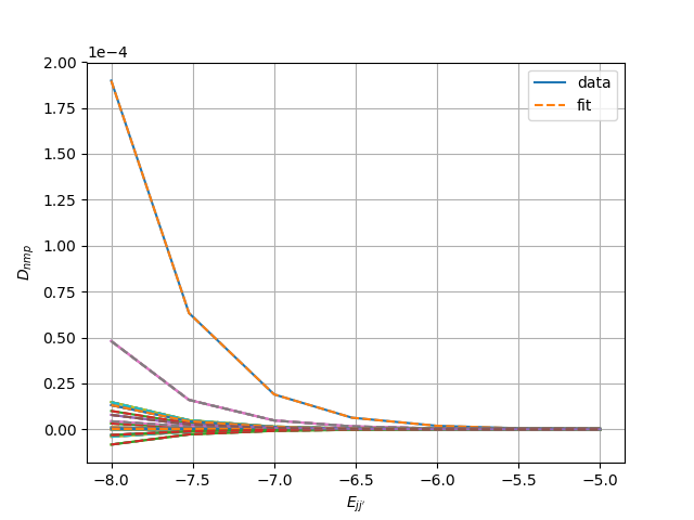
where we have made use of dependence of $E_{k}$ on $\vec{\xi}$ through Eqs. (3) and (31). This approximation also implicitly assumes $\vec{v}_{sa}\approx\vec{v}_{s}$ , since the argument of the basis function is $\vec{\xi}$ , hence independent of the ion/atom velocity $\vec{v}_{a}$ . Linearly factoring $f_{jj^{\prime}}$ in Eq. (25) would not be possible if we use generalized oscillator strengths, since $f_{jj^{\prime}}$ would then depend on the particle momentum transfer, as in Eq. (12). As we will see numerically in Section 3, in the limit $E_{jj^{\prime}}\ll E_{k}$ for all level pairs $(j,j^{\prime})$ , given Eq. (15) is inversely proportional to $E_{jj^{\prime}}$ to leading order, $\log(D_{n^{\prime\prime},m^{\prime\prime},p^{\prime\prime}}(E_{jj^{\prime}}))$ is very close to being linear in $\log(E_{jj^{\prime}})$ . This permits us to store $D_{n^{\prime\prime},m^{\prime\prime},p^{\prime\prime}}(E_{jj^{\prime}})$ as a set of two-parameter values that fit linear functions in this log space. Furthermore, the symmetry in radial velocity of the original kernel implies that $D_{n^{\prime\prime},m^{\prime\prime},p^{\prime\prime}}$ is invariant under permutations of $(n^{\prime\prime},m^{\prime\prime},p^{\prime\prime})$ , which permits further savings in data storage.

Incorporating Eq. (25) into the first and second terms of Eq. (24),

\frac{\partial C_{n^{\prime},m^{\prime},p^{\prime}}}{\partial t}=\sum_{n,m,p}C_{n,m,p}\left[\sum_{n^{\prime\prime},m^{\prime\prime},p^{\prime\prime}}f_{jj^{\prime}}D_{n^{\prime\prime},m^{\prime\prime},p^{\prime\prime}}(E_{jj^{\prime}})\;\;*\right.\\ \left\{\int f_{a,j}(\vec{v}_{a}^{\prime})d^{3}\vec{v}_{a}^{\prime}\int\Psi^{n^{\prime},m^{\prime},p^{\prime}}\left(\frac{1}{m_{e}+M_{a}}\left(m_{e}\vec{\xi}^{\prime}-M_{a}\vec{u}\oslash\vec{\alpha}\right)\right)\Psi_{n^{\prime\prime},m^{\prime\prime},p^{\prime\prime}}(\vec{\xi}^{\prime})\Psi_{n,m,p}(\vec{\xi}^{\prime})d^{3}\vec{\xi}^{\prime}\right.\\ \left.\left.-\int f_{a,j^{\prime}}(\vec{v}_{a})d^{3}\vec{v}_{a}\int\Psi^{n^{\prime},m^{\prime},p^{\prime}}(\vec{\xi})\Psi_{n^{\prime\prime},m^{\prime\prime},p^{\prime\prime}}(\vec{\xi})\Psi_{n,m,p}(\vec{\xi})d^{3}\vec{\xi}\right\}\right]\;\;,

(26)

where, given the preceding approximation, the integrals over $\beta$ -velocity and atom/ion velocity are separable, hence factored here. We have also used $\sigma_{j^{\prime}j}(E_{jj^{\prime}})=\sigma_{jj^{\prime}}(E_{jj^{\prime}})$ , under the assumption that permuting the initial and final energy levels does not change the cross section structure (statistical weights from partition functions factoring in the ion distributions, $f_{a,j}$ , break the equality for rates, however).

Given $m_{e}\ll M_{a}$ , the next approximation we might make is $\Psi^{n^{\prime},m^{\prime},p^{\prime}}\left(\left(m_{e}\vec{\xi}^{\prime}-M_{a}\vec{u}\oslash\vec{\alpha}\right)/(m_{e}+M_{a})\right)\approx\Psi^{n^{\prime},m^{\prime},p^{\prime}}(-\vec{u}\oslash\vec{\alpha})$ , which gives

\frac{\partial C_{n^{\prime},m^{\prime},p^{\prime}}}{\partial t}=\sum_{n,m,p}C_{n,m,p}\left[\sum_{n^{\prime\prime},m^{\prime\prime},p^{\prime\prime}}f_{jj^{\prime}}D_{n^{\prime\prime},m^{\prime\prime},p^{\prime\prime}}(E_{jj^{\prime}})\;\;*\right.\\ \left\{\Psi^{n^{\prime},m^{\prime},p^{\prime}}(-\vec{u}\oslash\vec{\alpha})\int f_{a,j}(\vec{v}_{a}^{\prime})d^{3}\vec{v}_{a}^{\prime}\int\Psi^{0,0,0}(\xi^{\prime})\Psi_{n^{\prime\prime},m^{\prime\prime},p^{\prime\prime}}(\vec{\xi}^{\prime})\Psi_{n,m,p}(\vec{\xi}^{\prime})d^{3}\vec{\xi}^{\prime}\right.\\ \left.\left.-\int f_{a,j^{\prime}}(\vec{v}_{a})d^{3}\vec{v}_{a}\int\Psi^{n^{\prime},m^{\prime},p^{\prime}}(\vec{\xi})\Psi_{n^{\prime\prime},m^{\prime\prime},p^{\prime\prime}}(\vec{\xi})\Psi_{n,m,p}(\vec{\xi})d^{3}\vec{\xi}\right\}\right]\;\;,

(27)

where we have inserted $\Psi^{0,0,0}(\xi^{\prime})=1$ in the integral, in order to show it is now a special case of the second pre-scatter integral. For more generality, we could have expanded $\Psi^{n^{\prime},m^{\prime},p^{\prime}}\left(\left(m_{e}\vec{\xi}^{\prime}-M_{a}\vec{u}\oslash\vec{\alpha}\right)/(m_{e}+M_{a})\right)$ in terms of the upper-index form of the basis, but this does not add significant formulaic complication (but it does complicate numerical computation).

The triple-basis integrals in Eq. (27) are separable by dimension in Cartesian velocity space, resulting in three integrals, where each has an integrand that is a product of three Hermite basis functions: one upper-index and two lower-index. For two upper-index and one lower-index Hermite basis, the solution of the integral has been developed via use of a 3-dimensional generator function by Askey et al. (1999). To evaluate the one upper-index, two lower-index integral, we may revisit the generator function approach given by Askey et al. (1999), to find a closed-form finite sum that embeds the two upper-index, one lower-index version of the function. We provide this derivation in Appendix B, and using the result, Eq. (B21), Eq. (27) becomes

\frac{\partial C_{n^{\prime},m^{\prime},p^{\prime}}}{\partial t}=\sum_{n,m,p}C_{n,m,p}\left[\sum_{n^{\prime\prime},m^{\prime\prime},p^{\prime\prime}}f_{jj^{\prime}}D_{n^{\prime\prime},m^{\prime\prime},p^{\prime\prime}}(E_{jj^{\prime}})\;\;*\right.\\ \left\{\Psi^{n^{\prime},m^{\prime},p^{\prime}}(-\vec{u}\oslash\vec{\alpha})\left(\int f_{a,j}(\vec{v}_{a}^{\prime})d^{3}\vec{v}_{a}^{\prime}\right)T_{c}(n,0,n^{\prime\prime})T_{c}(m,0,m^{\prime\prime})T_{c}(p,0,p^{\prime\prime})\right.\\ \left.\left.-\left(\int f_{a,j^{\prime}}(\vec{v}_{a})d^{3}\vec{v}_{a}\right)T_{c}(n,n^{\prime},n^{\prime\prime})T_{c}(m,m^{\prime},m^{\prime\prime})T_{c}(p,p,p^{\prime\prime})\right\}\right]\;\;.

(28)

If we are given the ion distribution $f_{a,j}(\vec{v}_{a})$ for all $j$ and fitting coefficients for $D_{n,m,p}$ , we may evaluate the matrix by summing over all pairs $(j,j^{\prime})$ to get the spectral formulation of Eq. (17). Moreover, the ion velocity integrals merely result in the population density for states $j$ and $j^{\prime}$ , $N_{a,j}$ and $N_{a,j^{\prime}}$ . The result is

\frac{\partial C_{n^{\prime},m^{\prime},p^{\prime}}}{\partial t}=\sum_{n,m,p}C_{n,m,p}\Biggl{[}\sum_{n^{\prime\prime},m^{\prime\prime},p^{\prime\prime}}\left\{\Psi^{n^{\prime},m^{\prime},p^{\prime}}(-\vec{u}\oslash\vec{\alpha})D_{n^{\prime\prime},m^{\prime\prime},p^{\prime\prime}}^{(U)}(\vec{x},t)T_{c}(n,0,n^{\prime\prime})T_{c}(m,0,m^{\prime\prime})T_{c}(p,0,p^{\prime\prime})\right.\\ \left.-D_{n^{\prime\prime},m^{\prime\prime},p^{\prime\prime}}^{(L)}(\vec{x},t)T_{c}(n,n^{\prime},n^{\prime\prime})T_{c}(m,m^{\prime},m^{\prime\prime})T_{c}(p,p,p^{\prime\prime})\right\}\Biggr{]}=\sum_{n,m,p}C_{n,m,p}S_{n,m,p}^{n^{\prime},m^{\prime},p^{\prime}}\;\;.

(29)

where


	$\displaystyle D_{n,m,p}^{(L)}(\vec{x},t)=\sum_{(j^{\prime},j)\in\mathcal{T}}N_{a,j^{\prime}}(\vec{x},t)f_{jj^{\prime}}D_{n,m,p}(E_{jj^{\prime}})\;\;,$		(30a)
	$\displaystyle D_{n,m,p}^{(U)}(\vec{x},t)=\sum_{(j^{\prime},j)\in\mathcal{T}}N_{a,j}(\vec{x},t)f_{jj^{\prime}}D_{n,m,p}(E_{jj^{\prime}})\;\;.$		(30b)

Similar to $D_{n,m,p}$ , the function $T_{c}(n,n^{\prime},n^{\prime\prime})$ is symmetric under permutation of $(n,n^{\prime},n^{\prime\prime})$ . Furthermore, $D_{n,m,p}$ and $T_{c}(n,n^{\prime},n^{\prime\prime})$ are spatially invariant functions; the ion distribution ultimately encodes spatial variation in the spectral scattering matrix. The spatial invariance and symmetry under index permutation make $D_{n,m,p}$ and $T_{c}(n,n^{\prime},n^{\prime\prime})$ , as well as the linear fitting representation of $D_{n,m,p}$ , very memory efficient in computational storage, compared to the spectral solution $C_{n,m,p}$ . For instance, considering the basis symmetry, for $(n,m,p)\in\{0,1,2,3,4\}^{3}$ , the number of $C_{n,m,p}$ values to store is 125 per spatial zone, while $T_{c}(n,m,p)$ results in at most 35 distinct floating point values, and $D_{n,m,p}$ results in 35 distinct pairs of floating point values (assuming two-parameter linear fits over atomic transition energy $E_{jj^{\prime}}$ , as discussed). The $T_{c}(n,m,p)$ function is also made asymptotically $\sim$ 50% sparse for large $(n,m,p)$ , by the $(n,m,p)$ parity selection rules discussed in Appendix B.

Specifically for Section 4, our final main approximation is to assume Maxwellian velocity dependence of the ion distribution $f_{a,j}(\vec{v}_{a})$ and Boltzmann statistics for excitation energy. This is a LTE assumption about the relative population of the excitation states within an ionization stage. While we also restrict our calculations to a single ion stage, we note that Saha statistics (hence the Saha-Boltzmann formulation, for instance as presented by Mihalas & Mihalas (1984)) can be used, without complicating the above matrix formulae. For more detail on the integrals using the Maxwellian ion distribution, as well as evaluation of the solid angle integral of the differential cross section, see Appendix A.

2.3 A general derivation outline

To end this section, we note that the calculation procedure described above may translate to a more general derivation sequence, applicable to different types of collision kernels. These general steps are outlined here.

1.

Identify the optimal coordinate system of velocity space to spectrally expand functional forms of the solution distribution and the differential cross section.
2.

Choose one or more spectral basis in the velocity coordinate system, based on physics (for example Gaussian weighting function for inner products, for natural scale-bridging, or relativity-compatible functions such as the Maxwell-Jüttner distribution) and physical regime, and expand both the distribution function and cross section in terms of the basis functions.
3.
Determine if parametric fits (for example, in this work over atomic transition energy) are applicable to the fundamental cross section coefficients ( $D_{n,m,p}$ ).
1. (a)
  
  Store the spatially invariant form of the parameterized coefficients if possible (for instance, excluding integration of the coefficient over the atom/ion distribution).
2. (b)
  
  Determine any index symmetries to further compress the $D_{n,m,p}$ array.
4.

Incorporate the expansions into the collision kernel relating the distribution to the differential cross section.
5.

Use the principle of micro-reversibility to (possibly) simplify evaluation of the post-scatter term.
6.

Determine if approximations, or an expansion, is possible to separate kernel integrals by species (for example, the separation of the integral over ion velocity above).
7.

Integrate and use basis orthogonality to arrive at a spectral matrix equation.
8.
If possible, use closed-form expressions for basis function triple-products (Askey et al., 1999).
1. (a)
  
  If the cross section and distribution use the same basis functions, it may be possible to follow the generator function procedure given by Askey et al. (1999) to find a closed form.
2. (b)
  
  If the cross section uses a different basis expansion (for example, Legendre polynomials), it may be possible to use a Gram-Schmidt orthonormalization procedure to express the polynomial factor of one basis in terms of the polynomial (upper-index) factor of the other.
3. (c)
  
  Determine any index symmetries to further compress pre-computation of the triple product function.
4. (d)
  
  Identify index selection rules that may increase sparsity of triple product function evaluation.

3 Numerical Verification of Spectral Collision Matrix

In this section, we numerically verify different aspects of the computation of the spectral collision matrix $S_{n,m,p}^{n^{\prime},n^{\prime},p^{\prime}}$ , in order to motivate the proof-of-principle 3D KN simulation presented in Section 4. First, we numerically verify the correctness of the compact triple Hermite products involving one upper-index basis and two lower-index basis functions. Next, we examine spectral expansions of the uncollided $\beta$ -particle distribution (or the emitted $\beta$ -particle distribution) and the fast-particle collision kernel. We then verify the two-parameter coefficient fits used for the closed-form expansion of the cross section match the direct calculation over different values of atomic transition energy. Finally, we compare direct numerical integration of Eq. (24) with the evaluation of Eq. (28). For all evaluations of the kernel or cross section, we assume a collision parameter of $\epsilon=10^{-3}$ in Eq. (A11), which corresponds to a minimum collision angle of $\sim 2.5^{\circ}$ . Importantly, in this and the following section, for expanding the $\beta$ -particle emission and cross sections, we initially transform the kinetic energy into radial velocity using the relativistic formula,

|\vec{v}|=c\sqrt{1-\left(\frac{1}{E_{k}/(m_{e}c^{2})+1}\right)^{2}}\;\;,

(31)

in order to systematically restrict the velocity domain to a more causal region of velocity space. However, the Hermite basis still extends beyond $|\vec{v}|=c$ .

In Table 1, we compare the closed form of the compact triple Hermite products (Appendix B, Eq. (B21)) to a direct 1024-point Midpoint Rule numerical integration over the non-dimensional velocity domain $\xi\in(-4,4)$ . We see very good agreement for all values, but an increased discrepancy at higher order basis functions. This seems to be due to the integral bounds in $\xi$ not being extended far enough for accuracy in the direct numerical integration (the bounds are supposed to be indefinite, $\xi\in(-\infty,\infty)$ ); as the bounds are increased the Midpoint Rule implementation comes into closer agreement with the closed form across modes.

	$T_{c}(0,0,0)$	$T_{c}(1,1,1)$	$T_{c}(1,2,3)$	$T_{c}(3,1,2)$
	$T_{c}(2,2,2)$	$T_{c}(4,0,0)$	$T_{c}(0,4,0)$	$T_{c}(4,4,4)$
Midpoint Rule	0.3989422804014322	0.0	0.043186768679	0.043186768679
	0.017630924480	0.0610753139878	0.0610753139878	0.001431449
Closed Form	0.3989422804014327	0.0	0.043186768684	0.043186768684
	0.017630924486	0.0610753139879	0.0610753139879	0.001431452

Table 1: Numerical values of compact triple Hermite products using 1024-point Midpoint Rule over

\xi\in(-4,4)

(first row) and the closed form presented in Appendix B. The function is symmetric under permutation of the three index arguments, corresponding to each basis order involved in the inner product.

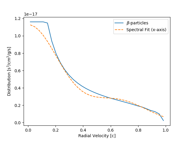
Turning to the spectral reconstruction of the uncollided $\beta$ -particle distribution and scatter angle-integrated collision kernel, some numerical experimentation indicates $\alpha_{x}=\alpha_{y}=\alpha_{z}=0.5c$ and $u_{x}=u_{y}=u_{z}=0$ are reasonable basis parameters for both. Figure 1 has a plot of the uncollided $\beta$ -particle distribution (solid blue), calculated from $\beta$ -particle emission spectrum , and a line-out of the spectrally reconstructed profile (dashed orange), using Eq. (2) with $n$ , $m$ , $p$ each ranging from 0 to 8 in Hermite basis order. We see some oscillation in the fit, which resembles the well-known Gibbs phenomenon (the ringing artefacts are near high curvature in the profile). The fit is poor for radial velocity below $\sim 0.2c$ , where the original distribution is set to a constant. This also is a range where the validity of the fast-particle quantum approximation may start to break down (Inokuti, 1971).

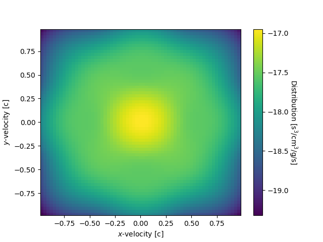
Refer to caption — Figure 1: Left: Reference uncollided $\beta$ -particle distribution (blue) and line-out of corresponding spectral reconstruction over 9x9x9 velocity basis functions (dashed orange), versus radial velocity. The original distribution is calculated from 0.2 $c$ , and is set to a constant for lower velocity. Right: Base-10 log of reconstructed uncollided $\beta$ -particle distribution versus $xy$ -plane of velocity space.

The left panel of Fig. 2 shows the original (solid) and reconstructed (dashed) kernel, where the reconstructed kernel is over the same 9x9x9 basis as in Fig. 1 (again with $\alpha_{x}=\alpha_{y}=\alpha_{z}=0.5c$ and $u_{x}=u_{y}=u_{z}=0$ ). Some oscillation can be seen in the reconstructed kernel as well, and coincidentally the fit is also poor at radial velocity below $\sim 0.2c$ , where error from the original kernel approximation may start to be significant. Furthermore, in the right panel of Fig. 2 is a plot of the base-10 log of the reconstructed kernel over the $xy$ -plane in velocity space. While the original kernel is radially symmetric, the reconstructed kernel shows artifacts from fitting over a Cartesian basis of Hermite functions.

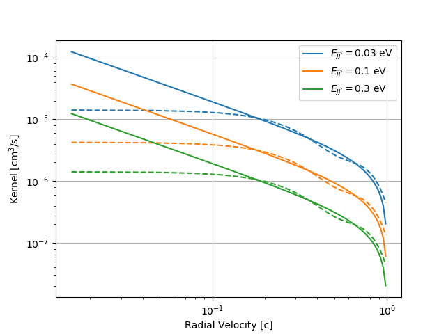
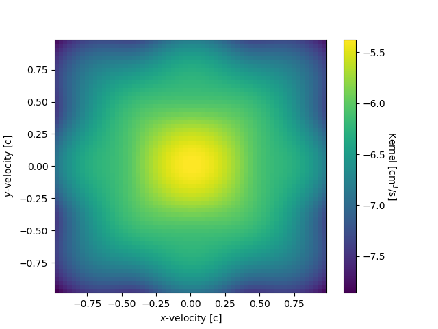
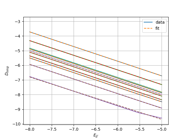
Figure 3 has $D_{n,m,p}$ versus a parameterized transition energy $E_{jj^{\prime}}$ , for a few selected values of $(n,m,p)$ , comparing direct evaluation of the expansion coefficients to linear fits in log-log space. We observe that the linear fits in log-log space do well to capture the dependence of each $D_{n,m,p}$ term for the range of atomic transition energies considered, $\sim$ 0.001 to 10 eV. For subsequent calculations involving construction of the spectral matrix, we use these fits to $D_{n,m,p}$ (which are particularly important for Section 4).

The Hermite basis reconstructions in Figs. 1 and 2 suggest orders 0 to 8 in each dimension may furnish reasonable accuracy, notwithstanding the approximations already made in the kernel and $\beta$ -particle emission. We now verify that these Hermite basis orders are sufficient for accuracy when incorporated into the pre-scatter portion of Eq. (27). To do so, we compare direct numerical integration of Eq. (24) to the evaluation of Eq. (28), for a single line with oscillator strength $f_{jj^{\prime}}=1$ and transition energy $E_{jj^{\prime}}=0.1$ eV. Table 2 has numerical values for some entries of the spectral scattering matrix, for direct integration by the Midpoint Rule on a $64^{3}$ point velocity domain and using Eq. (28), with either 5x5x5 or 9x9x9 Hermite basis functions. Also in Table 2 is relative error, as a fraction of the direct numerical integral. The matrix elements which are very close numerically to 0 have high error, but these terms will not contribute to the solution. Otherwise, for the significant entries, we see the low order values are in close agreement but along rows/columns of the matrix the error increases with higher disparity between modes, at $\sim$ 28% for the $S_{0,0,0}^{4,0,0}$ term using 5x5x5 basis functions. However, in using Eq. (28), we do not have to restrict the innermost sum to 5x5x5, even when simulating $C_{n,m,p}$ modes only up to 5x5x5. If we permit this innermost sum to go instead to 9 in each velocity dimension, we obtain results with systematically lower error relative to direct integration ( $\lesssim 10$ % for non-trivial modes). These results indicate that a 9x9x9 basis truncation of the innermost sum can accurately integrate the matrix terms, consistent with the accuracy of the profile of the truncated kernel expansion shown in Fig. 2.

	$S_{0,0,0}^{0,0,0}$	$S_{0,0,0}^{1,0,0}$	$S_{0,0,0}^{2,0,0}$	$S_{0,0,0}^{3,0,0}$	$S_{0,0,0}^{4,0,0}$
	$S_{2,0,0}^{0,0,0}$	$S_{2,0,0}^{1,0,0}$	$S_{2,0,0}^{2,0,0}$	$S_{2,0,0}^{3,0,0}$	$S_{2,0,0}^{4,0,0}$
	$S_{4,0,0}^{0,0,0}$	$S_{4,0,0}^{1,0,0}$	$S_{4,0,0}^{2,0,0}$	$S_{4,0,0}^{3,0,0}$	$S_{4,0,0}^{4,0,0}$
Midpoint Rule, Eq. (24)	-1.064612e-06	-2.244660e-24	3.773394e-07	-3.568146e-24	-1.838709e-07
	3.773394e-07	1.754513e-24	-4.477249e-07	1.501545e-25	3.166727e-07
	-1.838709e-07	2.815265e-25	3.166727e-07	5.027491e-25	-3.093139e-07
Eq. (28) (5x5x5 basis)	-1.035940e-06	8.427530e-24	3.404054e-07	-4.664180e-24	-1.332969e-07
	3.404054e-07	3.839731e-24	-3.996374e-07	2.175768e-24	2.853456e-07
	-1.332969e-07	-4.118894e-24	2.853456e-07	1.544883e-24	-2.920202e-07
Eq. (28) (9x9x9 basis)	-1.059921e-06	5.339311e-24	3.688633e-07	-6.485463e-26	-1.696097e-07
	3.688633e-07	7.438594e-24	-4.320753e-07	1.294707e-24	2.999444e-07
	-1.696097e-07	-5.558943e-24	2.999444e-07	1.526768e-24	-2.977645e-07
Error (5x5x5 basis)	0.02693188	4.75447952	0.09788005	0.30717185	0.27505168
	0.09788005	1.1884882	0.10740412	13.4901951	0.0989258
	0.27505168	15.63057297	0.0989258	2.07287074	0.05590987
Error (9x9x9 basis)	0.0044063	3.37867249	0.0224628	0.981824	0.07756094
	0.0224628	3.23969158	0.03495361	7.62249883	0.0528252
	0.07756094	20.74571843	0.0528252	2.03683885	0.03733877

Table 2: Numerical values of the pre-scatter portion of the spectral collision matrix, and relative errors as a fraction of numerical integral. The top three rows are from direct numerical integration of Eq. (24) over a 64³ point velocity domain using the Midpoint Rule. The next three rows are from evaluating Eq. (28) using compact triple Hermite products and the fitted data coefficients

D_{n,m,p}

, using 5x5x5 basis functions. The next three rows are again for Eq. (28), but using 9x9x9 basis functions. The bottom six rows are the relative error between the Midpoint Rule and Eq. (28), as a fraction of the Midpoint Rule.

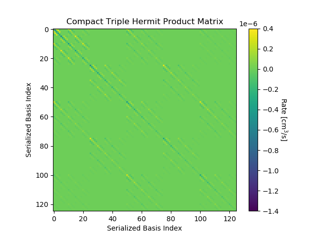
In what follows, we restrict our attention to the pre-scatter matrix, since the post-scatter matrix does not complicate the analysis. Again we assume a single line, a pre-scatter ion population density of 1 (effectively), an atomic transition energy of 0.1 eV, and an oscillator strength of 1. In Fig. 4, we show the full matrix for a 5x5x5 velocity basis functions versus serialized matrix indices. The left panel has the direct numerical integral of Eq. (24) for each matrix entry, again using a Midpoint rule over 64³ points in velocity space, and the right panel uses Eq. (28) for each matrix entry (hence using the closed form compact triple Hermite product functions). Even over the coarse velocity space grid, the cost of directly numerically integrating the pre-scatter matrix is significantly higher than using the compact triple Hermite product functions: 1743 seconds for the numerical integration and 2.2 (5.1) seconds for the 5x5x5 (9x9x9) innermost sum (using Python/NumPy on a single CPU). This time comparison is in fact for a sub-optimal implementation of the compact triple Hermite functions, where they are reevaluated for each instance they are invoked, rather than simply pre-computed. Moreover, the structure of the matrix matches between the two methods (for this kernel, we observe that much of the qualitative structure comes from the triple-products of the Hermite basis function, which can be seen by setting all the $D_{n,m,p}$ values to a constant and comparing to the matrix using detailed atomic data).

4 Simplified 3D KN ejecta thermalization trial calculation

In Section 3 we verify the important steps of computing the terms of the spectral matrix $S_{n,m,p}^{n^{\prime},m^{\prime},p^{\prime}}$ , which linearly couple together modes of the solution $C_{n,m,p}$ . We now apply the 9x9x9 basis functions used in Section 3, with the parameters $\vec{\alpha}=0.5$ and $\vec{u}=0$ , to a proof-of-principle KN model in 3D Cartesian spatial geometry. We use the MASS-APP code base, which is a spectral Hermite solver for the Vlasov-Maxwell-Boltzmann equations. The MASS-APP code non-dimensionalizes the equations following Eq. (C1); we leverage the reference plasma electron oscillation frequency in Eq. (C1) to match the expansion time scale of the KN, setting it to $5\times 10^{-5}$ radians/s. The physical length scale of KNe from 1 day to a week is $\sim 10^{14}-10^{15}$ cm, which implies the reference plasma oscillation frequency furnishes a non-dimensional length scale of O(1). Consequently, we set the 3D spatial domain to a $[-1,1]\times[-1,1]\times[-1,1]$ non-dimensional cube.

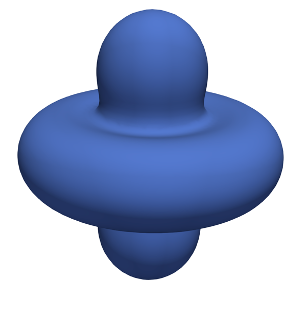
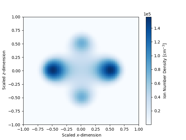
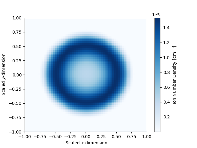
The KN model has an axisymmetric ejecta with a toroidal (T) component superimposed with lobed (P; “peanut”) component. The formula for the ion density is derived from the Cassini oval approach of Korobkin et al. (2021),

N_{a}(\bar{x},\bar{y},\bar{z})=N_{a,0}\begin{cases}(1-\bar{r}^{4}+4\bar{z}^{2}-2\bar{r}^{2})^{3}\;\;,\;\;\text{(T)}\;\;,\\ (1.5-\bar{r}^{4}-4\bar{z}^{2}+2\bar{r}^{2})^{3}\;\;,\;\;\text{(P)}\;\;,\end{cases}

(32)

where $N_{a,0}$ is number density, $\bar{x}$ , $\bar{y}$ , and $\bar{z}$ are scaled non-dimensional spatial Cartesian coordinates, and $\bar{r}^{2}=\bar{x}^{2}+\bar{y}^{2}+\bar{z}^{2}$ . We set the scaling to 2, so $\bar{\vec{r}}=2\tilde{\vec{r}}$ , where the components of $\tilde{\vec{r}}$ range from -1 to 1 and are non-dimensional in the form of Eq. C1. Considering the typical homologous approximation for KN (or supernova) ejecta, we see that the non-dimensionalization procedure implies,

\tilde{\vec{x}}=\frac{\vec{v}_{\rm exp}}{c}\tilde{t}_{\rm exp}\;\;,

(33)

where $\vec{v}_{\rm exp}$ is the bulk expansion velocity of the ejecta, and $\tilde{t}_{\rm exp}$ is the non-dimensional time elapsed since the merger event. A non-dimensional expansion time of 5 then corresponds to $10^{5}$ seconds of physical time, or about 1 day, which translates to a physical expansion velocity of 0.2 $c$ for $\tilde{x}=1$ , $\tilde{z}=\tilde{y}=0$ . This configuration effectively sets the ejecta velocity scale between the two components to be comparable (Korobkin et al., 2021).

We set the reference number density $N_{a,0}$ for the profile to $10^{4}$ cm^-3, which is very low, corresponding to an ejecta mass of $5\times 10^{-5}$ solar masses. This choice approximates the fraction of mass of Neodymium (Nd) in a more realistic total (see, for instance, Table 1 of Even et al. (2020)); Nd has a significant impact on the photon opacity (Even et al., 2020). The total density profile is a sum over the components where each component imposes a minimum background density of $N_{a,\min}=10^{-2}$ cm^-3,

N_{a,{\rm tot}}(\bar{x},\bar{y},\bar{z})=\max(N_{a,\min},N_{a,0}(1-\bar{r}^{4}+4\bar{z}^{2}-2\bar{r}^{2})^{3})+\max(N_{a,\min},N_{a,0}(1.5-\bar{r}^{4}-4\bar{z}^{2}+2\bar{r}^{2})^{3})\;\;.

(34)

Figure 5 has isocontour (top panel) and $zx$ , $xy$ -plane (bottom left and right panels) plots of the ion density given by Eq. (32), showing the shape of the combined ejecta components.

The ion temperature is assumed to be isothermal, or uniform in space (consistent with thermal electron temperature at late time in some LTE two-temperature KN simulations), and we set it to 0.1 eV. We make an extreme assumption that the entire ejecta is singly ionized Nd, and use energy levels ( $E_{j}$ ), statistical weights ( $g_{j}$ ), and oscillator strengths $f_{jj^{\prime}}$ from the LANL suite of atomic physics codes (Fontes et al., 2015b). We neglect oscillator strengths below $10^{-3}$ , leaving a total of 6888 levels, connected by 375026 lines. Within the singly ionized Nd stage, we determine the excitation levels with the Boltzmann factor and partition function,

\int f_{a,j}(\vec{v})d^{3}\vec{v}_{a}=N_{a,j}=\left(\frac{g_{j}e^{-E_{j0}/T_{a}}}{\sum_{j^{\prime}}g_{j^{\prime}}e^{-E_{j^{\prime}0}/T_{a}}}\right)N_{a}\;\;,

(35)

where $T_{a}$ is the ion temperature. Equation (35) is an assumption of LTE in the excitation states of the ion.

We simulate the model with 10 uniform time steps and 64³ spatial points over one second of physical time, using an initial condition for the $\beta$ -particle spectrum from Fig. 1, proportionally scaling with ejecta density $N_{a}$ to account for higher $\beta$ -emission rates at higher ion densities. The initial electromagnetic field is set to 0 everywhere ( $\vec{E}=\vec{B}=0$ ). On the AMD Rome EPYC 7H12 CPU partition of the HPC system Chicoma at LANL, the simulation took 1.4 hours on 256 cores (we recalculate the matrix entries each time step despite keeping the ion temperature and density as constant in time).

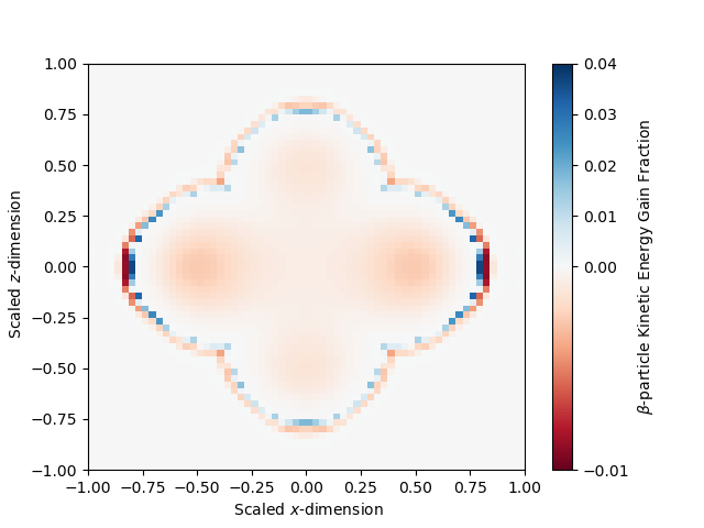
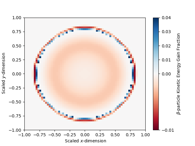
Figure 6 has the kinetic energy gain fraction at 1 second, relative to the initial conditions, in the $zx$ (left) and $xy$ (right) spatial planes. From these plots, we see the kinetic energy loss is enhanced in regions of high density in the ion field as expected, but we also observe a thin layer at the edge of the ejecta where a large fractional gain and loss occur. This effect may be attributable to a transitional region where the ion density is low enough that flux between zones begins to dominate over the collision matrix. We observe in this one second time scale that $\sim$ 0.3% ( $\sim$ 0.13%) of the initial kinetic energy in the $\beta$ -particle field is lost in density regions near the peak ion density of the torus (peanut) component.

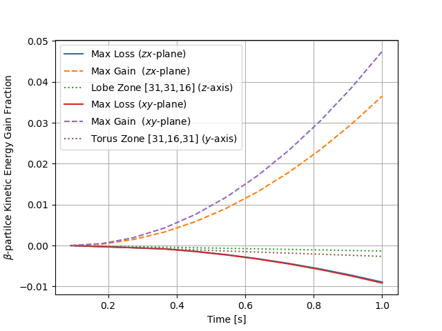
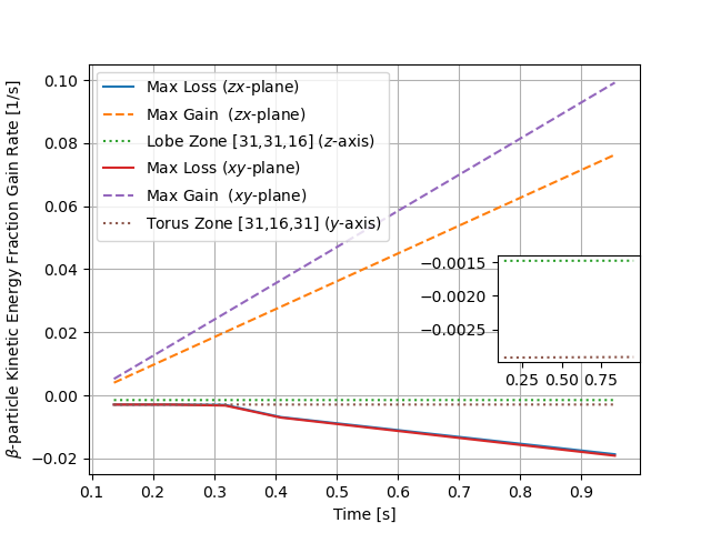
The left panel of Fig. 7 has fractional kinetic energy max gain (solid), max loss (dashed), and a selected torus/peanut zone versus time for the $zx$ and $xy$ -planes. We see that the fractional kinetic energy losses and gains near the outer edges are higher than losses in the torus and peanut lobes by a factor of a few and order of magnitude, respectively. It should be noted that these are spatially local fractional values; the energy lost in the torus and peanut lobe is orders of magnitude higher (the fractional metric happens to capture local behavior better, for instance exposing the effect at the ejecta boundary layer). The right panel of Fig. 7 has the corresponding rate of change (time derivative) of the left panel data. The rate of change in the fraction of kinetic energy lost to the ions, relative to the original amount in the spatial zone, is nearly constant over the second for torus and peanut lobe zones, at approximately 0.3% s^-1 and 0.15% s^-1 respectively, but grows in magnitude for the ejecta boundary layers. Assuming

\mathit{f}_{\beta,{\rm therm}}(t)\dot{\epsilon}_{k}(t)\approx\dot{\mathit{f}}_{\beta,{\rm therm}}(\epsilon_{k}(t)-\epsilon_{k}(0))\;\;,

(36)

where $\mathit{f}_{\beta,{\rm therm}}$ is the thermalization fraction and $\epsilon_{k}$ is the kinetic energy emitted by time $t$ , and given that we assumed an emissivity for the initial condition, such that $\epsilon_{k}(t)-\epsilon_{k}(0)=\dot{\epsilon}_{k}(t)$ , the rate of change in the fractions result in $\mathit{f}_{\beta,{\rm therm}}=0.003$ (T) or 0.0015 (P).

We may estimate the magnitude of the effect of excitation collision scattering angles $\geq 2.5^{\circ}$ relative to total $\beta$ -thermalization using the semi-analytic formulae of Barnes et al. (2016), in particular their Eqs. 20 and 32, reproduced here for convenience,


	$\displaystyle t_{\beta,{\rm ineff}}=7.4\left(\frac{E_{k}}{0.5\text{ MeV}}\right)^{-1/2}\left(\frac{M_{\rm ej}}{5\times 10^{-3}\text{ M}_{\odot}}\right)^{1/2}\left(\frac{\vec{v}_{\rm exp}}{0.2c}\right)^{-3/2}\text{days}\;\;,$		(37a)
	$\displaystyle\mathit{f}_{\beta,{\rm therm}}(t)=\frac{\ln(1+2(t/t_{\beta,{\rm ineff}})^{2})}{2(t/t_{\beta,{\rm ineff}})^{2}}\;\;,$		(37b)

where $t_{\beta,{\rm ineff}}$ is the time scale to inefficient thermalization, which happens to be about where the peak of the KN transient matches the thermalization time scale (Barnes et al., 2016), and $\mathit{f}_{\beta,{\rm therm}}$ is again the thermalization fraction at time $t$ , which multiplies the bare emission rate. Using the dimensional values of our 3D model, with $t=10^{5}$ s and $\vec{v}_{\rm exp}=0.1c$ , and obtaining an average uncollided $\beta$ -particle energy of 0.3 MeV from integrating $\int E_{k}f_{s}(E_{k})dE_{k}/\int f_{s}(E_{k})dE_{k}$ , we see the inefficiency time scale and thermalization fraction for the total $\beta$ -particle interaction should be roughly 2.7 days and 0.85, respectively. Compared to 0.85, the estimates of 0.003 (T) and 0.0015 (P) are much lower, corresponding to $\sim$ 0.03 days and $\sim$ 0.02 days inefficiency time scales, respectively (using the Newton-Raphson method on Eq. (37)b). This indicates excitation scattering at large angle is a sub-dominant but not vanishingly small mechanism for energy transfer to the ions. Incorporating large-angle ionization and free electron Coulomb collisions may increase the large-angle contribution to thermalization as well (Barnes et al., 2021). Alluded to earlier, a significant caveat to this numerical evaluation is that the fast-particle approximation has been built into our derivation for large angle scatters, which for lower energy $\beta$ -particles may become invalid.

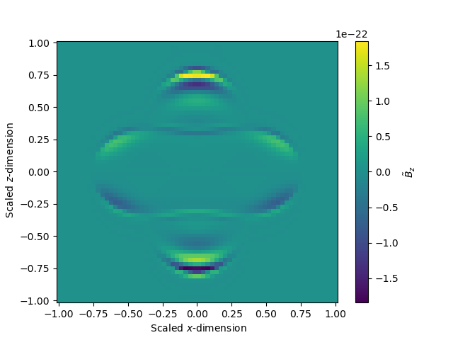
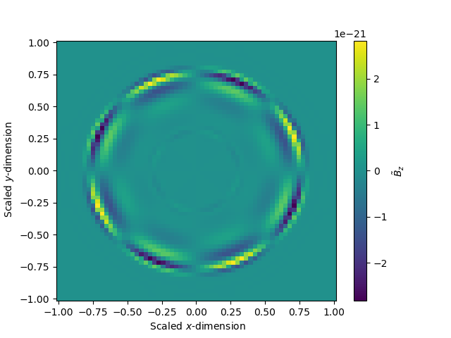
Given that the Maxwell equations are also being solved, and we started the simulation with $\vec{E}=\vec{B}=0$ , it may be of interest to see the structure of the magnetic field after one second. Figure 8 has the $z$ -component of the non-dimensional magnetic field in the $zx$ (left) and $xy$ (right) spatial planes. The non-dimensional magnetic field is very low, and nearly 0 everywhere except the edges, again indicating a region where particle flux, and hence current, is important. The non-zero portions show antisymmetry under reflection through the $xy$ -plane, consistent with the 0-divergence condition of the magnetic field. The alternating field in the $xy$ -plane suggests the formation of a very weak long-wavelength electromagnetic wave near the surface of the toroidal ejecta. We can see that these values of $\tilde{B}_{z}$ are subdominant to the collision matrix by examining $C_{0,1,0}$ , which corresponds to particle momentum in the $y$ -direction: the time rate of change of $C_{0,1,0}$ is proportional to $\tilde{B}_{z}C_{1,0,0}$ through the Lorentz force (see Eq. (C2)), but it is also proportional to $\sum_{n^{\prime},m^{\prime},p^{\prime}}S_{0,1,0}^{n^{\prime},m^{\prime},p^{\prime}}C_{n^{\prime},m^{\prime},p^{\prime}}$ , where the dominant values of $S_{0,1,0}^{n^{\prime},m^{\prime},p^{\prime}}$ are $\sim$ 14 orders of magnitude larger than $\tilde{B}_{z}$ . As a C-coefficient, the electric field is similarly orders of magnitude lower than the dominant collision matrix elements, but only by $\sim$ 4 orders of magnitude.

5 Conclusions

We have formulated and implemented a preliminary spectral evaluation of the fast-particle atomic excitation kernel presented by Inokuti (1971). The resulting spectral collision matrix couples basis orders in a spatially local way, and balances spatial flux and classical electromagnetic terms in the equation governing the time rate of change of the spectral modes. The formulation is restricted to the non-relativistic, fast-particle kernel, consistent with the Bethe-Born approximation (Bethe, 1930), and uses optical oscillator strength data as in photon-matter opacity calculations. This development has been done in the MASS-APP spectral solver framework, which uses Kokkos (Trott et al., 2021) for thread/GPU parallelism and FleCSI (Bergen et al., 2016) to support MPI or Legion-parallel task backends, each layer providing portability and performance on different HPC systems. The code has a full treatment of classical $\vec{E}$ and $\vec{B}$ fields, thus enabling efficient 3D calculations of KN ejecta $\beta$ -particle thermalization along with electromagnetic effects (which we did not explore with the kernel in this work).

We expand the cross section in terms of the Hermite basis, and find that the simple leading-order dependence of the cross section on atomic bound-bound level transition energy propagates to the expansion coefficients. Moreover, the symmetry of the kernel in radial velocity (in velocity space) imply these expansion coefficients are symmetric under permutation of the mode/order indices, and hence form a compressible low-cost data structure for computer memory when fitted to linear functions in log-coefficient-log-transition energy space. Similarly, the compact triple Hermite product functions, which build the elements of the spectral scattering matrix, are symmetric under permutation of the mode/order indices, and obey mode/order parity-based index selection rules that make them sparse. These compact triple Hermite product functions also permit interoperability of the spectral collision matrix with adaptive basis coefficients, though we do not test this here.

Numerical results indicate that a reasonable choice of Hermite basis parameters for $\beta$ -particles in the KN are a bulk velocity parameter $\vec{u}=0$ , a thermal velocity parameter $\vec{\alpha}=0.5c$ , and a 9x9x9 mode velocity basis set (Hermite orders 0 to 8 in each dimension). Section 3 verifies each step in the computation of the spectral collision matrix by comparing compact Hermite triple product functions and matrix elements to the equivalent direct numerical quadrature of the corresponding integrals. Furthermore, in Section 3 we demonstrate the ability to fit the coefficients of the fast-particle cross section Hermite expansion with linear functions, a property inherited from the leading-order behavior of the differential cross section for small ratios of excitation energy to $\beta$ -particle kinetic energy. With an implementation of the spectral collision matrix in MASS-APP, we show a proof of principle calculation of $\beta$ -particle propagation and excitation interaction in a 3D snapshot simulation of KN ejecta. Given a lower bound scattering angle of $\sim 2.5^{\circ}$ and the caveat of the fast-particle approximation (for instance, using the limit of optical oscillator strengths), this calculation suggests that large-angle scatters of $\beta$ -particles may not be more than three orders of magnitude lower as a power source for the KN luminosity and spectra, not including ionization and free electron Coulomb contributions.

With some further work, the framework should extend to generalized oscillator strengths and the relativistic kernel given by Inokuti (1971), with the caveat that it may be important to replace the Hermite basis with a causally restricted basis (bounding velocity by the speed of light), for instance using Legendre polynomials as done by Manzini et al. (2017). Another consideration for velocity space is the coordinate system over which the basis functions are expressed. The uncollided $\beta$ -particle distribution and collision cross section are spherically symmetric in velocity space (though technically, the collision cross section is symmetric about the origin of the center-of-mass frame for each collision), so basis functions in spherical velocity coordinates (for instance, spherical harmonics) may further reduce the size of the basis expansion required for accurate solutions.

Another improvement to fidelity would be to use the homologous expansion velocity of the KN ejecta as the value of the bulk velocity parameter $\vec{u}$ in the basis functions, but this may be generally of negligible effect (Barnes et al., 2016). Since $\vec{u}$ is variable in space-time, this would require a modification to the standard spectral system to account for the variation in the equations, but varying the thermal ( $\vec{\alpha}$ ) and bulk velocity parameters is an active topic of research (Bessemoulin-Chatard & Filbet, 2023; Pagliantini et al., 2023). This would capture some effect of the expansion velocity in the $\beta$ -particle simulation, permitting a Galilean frame transformation of the kernel.

After adding Coulomb and ionization interactions to the spectral collision matrix, and incorporating both bulk ejecta and microphysical relativistic effects in the kernel, we ultimately intend to use MASS-APP to perform detailed thermalization calculations for $\beta$ -particles in KN ejecta, subject to different $\vec{E}$ and $\vec{B}$ field seeds, and use the results to power photon transfer simulations that synthesize observable light curves and spectra, following Barnes et al. (2021).

Finally, the efficient representation of the coefficients of the Hermite expansion of the cross section as linear in log-log space with respect to atomic transition energy suggests that other cross section formulae may conform at least approximately to an efficient representation over quantum atomic parameters.

This work was supported by the U.S. Department of Energy through the Los Alamos National Laboratory. Los Alamos National Laboratory is operated by Triad National Security, LLC, for the National Nuclear Security Administration of the U.S. Department of Energy (Contract No. 89233218CNA000001). Research presented in this article was supported by the Laboratory Directed Research and Development program of Los Alamos National Laboratory under project number 20220104DR. This research used resources provided by the Los Alamos National Laboratory Institutional Computing Program, which is supported by the U.S. Department of Energy National Nuclear Security Administration under Contract No. 89233218CNA000001.

Appendix A Kernel integral evaluation and approximation

A.1 Maxwellian integral evaluation

For completeness, we give details for evaluating the integral over atom/ion velocity here. We do not assume $\vec{v}_{sa}=\vec{v}_{s}$ , but instead show how the same result can be obtained after evaluating the integral over $\vec{v}_{a}$ . Assuming the pre-/post-collision atom/ion distribution is Maxwellian, and that the comoving collision integral is independent of ion/atom velocity, the ion/atom-dependent velocity integral is

\int|\vec{v}_{a}-\vec{v}_{s}|e^{-M_{a}v_{a}^{2}/2k_{B}T}d^{3}\vec{v}_{a}=2\pi\int_{0}^{\infty}\int_{-1}^{1}v_{sa}^{3}e^{-M_{a}(v_{sa}^{2}+2v_{sa}v_{s}\eta+v_{s}^{2})/2k_{B}T}d\eta dv_{sa}\;\;,

(A1)

where $\eta$ is the cosine of the angle between vectors $\vec{v}_{sa}$ and $\vec{v}_{s}$ , and the integral on the right side is over spherical coordinates. Integrating first over $\eta$ ,

2\pi\int_{0}^{\infty}\int_{-1}^{1}v_{sa}^{3}e^{-M_{a}(v_{sa}^{2}-2v_{sa}v_{s}\eta+v_{s}^{2})/2k_{B}T}d\eta dv_{sa}=2\pi\int_{0}^{\infty}v_{sa}^{3}e^{-M_{a}(v_{sa}^{2}+v_{s}^{2})/2k_{B}T}\left(\int_{-1}^{1}e^{M_{a}v_{sa}v_{s}\eta/k_{B}T}d\eta\right)dv_{sa}\\ =2\pi\int_{0}^{\infty}v_{sa}^{3}e^{-M_{a}(v_{sa}^{2}+v_{s}^{2})/2k_{B}T}\left(\frac{2k_{B}T}{M_{a}v_{sa}v_{s}}\sinh\left(\frac{M_{a}v_{sa}v_{s}}{k_{B}T}\right)\right)dv_{sa}\\ =\frac{4\pi k_{B}T}{M_{a}v_{s}}\int_{0}^{\infty}v_{sa}^{2}e^{-M_{a}(v_{sa}^{2}+v_{s}^{2})/2k_{B}T}\sinh\left(\frac{M_{a}v_{sa}v_{s}}{k_{B}T}\right)dv_{sa}\;\;.

(A2)

Expressing the hyperbolic sine in terms of exponentials, and completing the squares in the exponents,

\frac{4\pi k_{B}T}{M_{a}v_{s}}\int_{0}^{\infty}v_{sa}^{2}e^{-M_{a}(v_{sa}^{2}+v_{s}^{2})/2k_{B}T}\frac{1}{2}\left(e^{M_{a}v_{sa}v_{s}/k_{B}T}-e^{-M_{a}v_{sa}v_{s}/k_{B}T}\right)dv_{sa}\\ =\frac{2\pi k_{B}T}{M_{a}v_{s}}\int_{0}^{\infty}\left(v_{sa}^{2}e^{-M_{a}(v_{sa}-v_{s})^{2}/2k_{B}T}-v_{sa}^{2}e^{-M_{a}(v_{sa}+v_{s})^{2}/2k_{B}T}\right)dv_{sa}\;\;,

(A3)

where the rightmost integral can be re-expressed as

\int_{0}^{\infty}\left(v_{sa}^{2}e^{-M_{a}(v_{sa}-v_{s})^{2}/2k_{B}T}-v_{sa}^{2}e^{-M_{a}(v_{sa}+v_{s})^{2}/2k_{B}T}\right)dv_{sa}\\ =\int_{-v_{s}}^{\infty}(v+v_{s})^{2}e^{-M_{a}v^{2}/2k_{B}T}dv-\int_{v_{s}}^{\infty}(v-v_{s})^{2}e^{-M_{a}v^{2}/2k_{B}T}dv\\ =\int_{-v_{s}}^{v_{s}}v^{2}e^{-M_{a}v^{2}/2k_{B}T}dv+v_{s}^{2}\int_{-v_{s}}^{v_{s}}e^{-M_{a}v^{2}/2k_{B}T}dv+2v_{s}\left(\int_{-v_{s}}^{\infty}ve^{-M_{a}v^{2}/2k_{B}T}dv+\int_{v_{s}}^{\infty}ve^{-M_{a}v^{2}/2k_{B}T}dv\right)\;\;,

(A4)

using the substitution $v=v_{sa}-v_{s}$ ( $v=v_{sa}+v_{s}$ ) in the integral over the first (second) term. Using


	$\displaystyle\int_{-v_{s}}^{v_{s}}e^{-Cv^{2}}dv=\sqrt{\frac{\pi}{C}}\operatorname{erf}(\sqrt{C}v_{s})\;\;,$		(A5a)
	$\displaystyle\int_{-v_{s}}^{v_{s}}ve^{-Cv^{2}}dv=0\;\;,$		(A5b)
	$\displaystyle 2\int_{v_{s}}^{\infty}ve^{-Cv^{2}}dv=\frac{1}{C}e^{-Cv_{s}^{2}}\;\;,$		(A5c)
	$\displaystyle\int_{-v_{s}}^{v_{s}}v^{2}e^{-Cv^{2}}dv=\frac{1}{2C}\sqrt{\frac{\pi}{C}}\operatorname{erf}(\sqrt{C}v_{s})-\frac{v_{s}}{C}e^{-Cv_{s}^{2}}\;\;,$		(A5d)

Eq. (A4) further reduces to

\int_{0}^{\infty}\left(v_{sa}^{2}e^{-M_{a}(v_{sa}-v_{s})^{2}/2k_{B}T}-v_{sa}^{2}e^{-M_{a}(v_{sa}+v_{s})^{2}/2k_{B}T}\right)dv_{sa}\\ =\int_{-v_{s}}^{v_{s}}v^{2}e^{-M_{a}v^{2}/2k_{B}T}dv+v_{s}^{2}\int_{-v_{s}}^{v_{s}}e^{-M_{a}v^{2}/2k_{B}T}dv+2v_{s}\left(\int_{-v_{s}}^{\infty}ve^{-M_{a}v^{2}/2k_{B}T}dv+\int_{v_{s}}^{\infty}ve^{-M_{a}v^{2}/2k_{B}T}dv\right)\\ =\frac{k_{B}T}{M_{a}}\sqrt{\frac{2\pi k_{B}T}{M_{a}}}\operatorname{erf}\left(\sqrt{\frac{M_{a}}{2k_{B}T}}v_{s}\right)-\frac{2k_{B}Tv_{s}}{M_{a}}e^{-M_{a}v_{s}^{2}/2k_{B}T}+v_{s}^{2}\sqrt{\frac{2\pi k_{B}T}{M_{a}}}\operatorname{erf}\left(\sqrt{\frac{M_{a}}{2k_{B}T}}v_{s}\right)+2v_{s}\frac{2k_{B}T}{M_{a}}e^{-M_{a}v_{s}^{2}/2k_{B}T}\\ =\sqrt{\frac{2\pi k_{B}T}{M_{a}}}\left(\frac{k_{B}T}{M_{a}}+v_{s}^{2}\right)\operatorname{erf}\left(\sqrt{\frac{M_{a}}{2k_{B}T}}v_{s}\right)+\frac{2k_{B}Tv_{s}}{M_{a}}e^{-M_{a}v_{s}^{2}/2k_{B}T}\;\;.

(A6)

Incorporating Eq. (A6) into Eq. (A1) (via Eqs. (A2) and (A3)),

\int|\vec{v}_{a}-\vec{v}_{s}|e^{-M_{a}v_{a}^{2}/2k_{B}T}d^{3}\vec{v}_{a}\\ =\frac{2\pi k_{B}T}{M_{a}v_{s}}\left(\sqrt{\frac{2\pi k_{B}T}{M_{a}}}\left(\frac{k_{B}T}{M_{a}}+v_{s}^{2}\right)\operatorname{erf}\left(\sqrt{\frac{M_{a}}{2k_{B}T}}v_{s}\right)+\frac{2k_{B}Tv_{s}}{M_{a}}e^{-M_{a}v_{s}^{2}/2k_{B}T}\right)\\ =\left(\frac{2\pi k_{B}T}{M_{a}}\right)^{3/2}\frac{1}{v_{s}}\left(\frac{k_{B}T}{M_{a}}+v_{s}^{2}\right)\operatorname{erf}\left(\sqrt{\frac{M_{a}}{2k_{B}T}}v_{s}\right)+4\pi\left(\frac{k_{B}T}{M_{a}}\right)^{2}e^{-M_{a}v_{s}^{2}/2k_{B}T}\\ =\left(\frac{2\pi k_{B}T}{M_{a}}\right)^{3/2}\overline{\Lambda}_{a}(v_{s},T)\;\;,

(A7)

where we have introduced the function $\overline{\Lambda}_{a}(v_{s},T)$ , which represents the atom/ion distribution-weighted average magnitude of difference in velocity between the $\beta$ -particle and the atom/ions. When $v_{s}\gg\sqrt{k_{B}T/M_{a}}$ , Eq. (A7) simplifies to

\overline{\Lambda}_{a}(v_{s},T)\approx\frac{1}{v_{s}}\left(\frac{k_{B}T}{M_{a}}+v_{s}^{2}\right)\approx v_{s}\;\;.

(A8)

Thus, we have obtained the inverse of the Maxwellian normalization factor times the magnitude of the $\beta$ -particle velocity, as desired.

A.2 Solid angle integral of cross section

In Section 2, we factor the differential cross section out of the integral over atom/ion velocity, which can be evaluated as

\int\frac{d\sigma_{jj^{\prime}}}{d\Omega}d\Omega=4\pi f_{jj^{\prime}}\left(\frac{e^{2}}{4E_{k}}\right)^{2}\left(\frac{E_{k}}{E_{jj^{\prime}}}\right)\int_{\theta_{\min}}^{\pi}\csc^{4}(\theta/2)\left[1-\frac{1}{2}\left(\frac{E_{jj^{\prime}}}{E_{k}}\right)-\left(\sqrt{1-\left(\frac{E_{jj^{\prime}}}{E_{k}}\right)}\right)\cos(\theta)\right]\sin(\theta)d\theta\;\;,

(A9)

where $\theta_{\min}$ is a minimum scattering angle, which in general may depend on $E_{jj^{\prime}}$ (but we set it to a constant in this work). Making use of


	$\displaystyle\int_{\theta_{\min}}^{\pi}\csc^{4}(\theta/2)\sin(\theta)d\theta=4\int_{-1}^{1-\varepsilon}\frac{d\mu}{(1-\mu)^{2}}=4\left(\frac{1}{\varepsilon}-\frac{1}{2}\right)\;\;,$		(A10a)
	$\displaystyle\int_{\theta_{\min}}^{\pi}\csc^{4}(\theta/2)\cos(\theta)\sin(\theta)d\theta=4\int_{-1}^{1-\varepsilon}\frac{\mu d\mu}{(1-\mu)^{2}}=4\left(\frac{1-\varepsilon}{\varepsilon}+\frac{1}{2}+\ln(\varepsilon/2)\right)\;\;,$		(A10b)

where $\mu=\cos(\theta)$ and $1-\varepsilon=\cos(\theta_{\min})$ , Eq. (A9) becomes

\int\frac{d\sigma_{jj^{\prime}}}{d\Omega}d\Omega=\sigma_{jj^{\prime}}(v_{s})=\\ 8\pi f_{jj^{\prime}}\left(\frac{e^{2}}{2mv_{s}^{2}}\right)^{2}\left\{\left[\left(\frac{mv_{s}^{2}}{E_{jj^{\prime}}}\right)-1\right]\left(\frac{1}{\varepsilon}-\frac{1}{2}\right)-\left[\left(\frac{mv_{s}^{2}}{E_{jj^{\prime}}}\right)\sqrt{1-\left(\frac{2E_{jj^{\prime}}}{mv_{s}^{2}}\right)}\right]\left(\frac{1-\varepsilon}{\varepsilon}+\frac{1}{2}+\ln(\varepsilon/2)\right)\right\}\;\;,

(A11)

where we have used $E_{k}=m|\vec{v}_{s}-\overline{\vec{v}}_{a}|^{2}/2=mv_{s}^{2}/2$ .

Appendix B Derivation of compact Hermite triple products

B.1 Kernel expansion and standard triple-Hermite product

Expanding the pre-scatter kernel function, written with explicit dependence on a transition energy, in the upper-index basis,

S_{c}^{\rm(pre)}(v_{s},E_{jj^{\prime}})\approx\sum_{i_{x}^{\prime\prime},i_{y}^{\prime\prime},i_{z}^{\prime\prime}}^{I_{x},I_{y},I_{z}}\Psi^{i_{x}^{\prime\prime},i_{y}^{\prime\prime},i_{z}^{\prime\prime}}(\vec{\xi}_{s})\mathcal{D}_{i_{x}^{\prime\prime},i_{y}^{\prime\prime},i_{z}^{\prime\prime}}(E_{jj^{\prime}})\;\;,

(B1)

where $\mathcal{D}_{i_{x}^{\prime\prime},i_{y}^{\prime\prime},i_{z}^{\prime\prime}}(E_{jj^{\prime}})$ depends on transition energy but not on $\beta$ -particle speed $v_{s}$ . Incorporating Eq. (B1) into the integral for the spectral matrix elements,

S_{i_{x}^{\prime},i_{y}^{\prime},i_{z}^{\prime}}^{i_{x},i_{y},i_{z}\rm(pre)}=\int\Psi^{i_{x},i_{y},i_{z}}(\vec{\xi}_{s})S_{c}^{\rm(pre)}(v_{s},E_{jj^{\prime}})\Psi_{i_{x}^{\prime},i_{y}^{\prime},i_{z}^{\prime}}(\vec{\xi}_{s})d^{3}\vec{\xi}_{s}\\ =\sum_{i_{x}^{\prime\prime},i_{y}^{\prime\prime},i_{z}^{\prime\prime}}^{I_{x},I_{y},I_{z}}\mathcal{D}_{i_{x}^{\prime\prime},i_{y}^{\prime\prime},i_{z}^{\prime\prime}}(E_{jj^{\prime}})\int\Psi^{i_{x},i_{y},i_{z}}(\vec{\xi}_{s})\Psi^{i_{x}^{\prime\prime},i_{y}^{\prime\prime},i_{z}^{\prime\prime}}(\vec{\xi}_{s})\Psi_{i_{x}^{\prime},i_{y}^{\prime},i_{z}^{\prime}}(\vec{\xi}_{s})d^{3}\vec{\xi}_{s}\;\;.

(B2)

Using the standard formulae,


	$\displaystyle\psi^{i_{q}}(\xi_{q})=\frac{1}{\sqrt{2^{i_{q}}i_{q}!}}H_{i_{q}}(\xi_{q})\;\;,$		(B3a)
	$\displaystyle\psi_{i_{q}}(\xi_{q})=\frac{1}{\sqrt{\pi 2^{i_{q}}i_{q}!}}H_{i_{q}}(\xi_{q})e^{-\xi_{q}^{2}}=\frac{1}{\sqrt{\pi}}\psi^{i_{q}}(\xi_{q})e^{-\xi_{q}^{2}}\;\;,$		(B3b)
	$\displaystyle\Psi^{i_{x},i_{y},i_{z}}(\vec{\xi}_{s})=\psi^{i_{x}}(\xi_{x})\psi^{i_{y}}(\xi_{y})\psi^{i_{z}}(\xi_{z})\;\;,$		(B3c)
	$\displaystyle\Psi_{i_{x},i_{y},i_{z}}(\vec{\xi}_{s})=\psi_{i_{x}}(\xi_{x})\psi_{i_{y}}(\xi_{y})\psi_{i_{z}}(\xi_{z})\;\;,$		(B3d)

where $q$ denotes $x$ , $y$ , or $z$ , $H_{i_{q}}$ is the Hermite polynomial of order $i_{q}$ , and $\vec{\xi}_{s}=(\xi_{x},\xi_{y},\xi_{z})$ . Incorporating Eqs. (B3) into the right side of Eq. (B2),

S_{i_{x}^{\prime},i_{y}^{\prime},i_{z}^{\prime}}^{i_{x},i_{y},i_{z}\rm(pre)}=\sum_{i_{x}^{\prime\prime},i_{y}^{\prime\prime},i_{z}^{\prime\prime}}^{I_{x},I_{y},I_{z}}\mathcal{D}_{i_{x}^{\prime\prime},i_{y}^{\prime\prime},i_{z}^{\prime\prime}}(E_{jj^{\prime}})\int\Psi^{i_{x},i_{y},i_{z}}(\vec{\xi}_{s})\Psi^{i_{x}^{\prime\prime},i_{y}^{\prime\prime},i_{z}^{\prime\prime}}(\vec{\xi}_{s})\Psi_{i_{x}^{\prime},i_{y}^{\prime},i_{z}^{\prime}}(\vec{\xi}_{s})d^{3}\vec{\xi}_{s}\\ =\sum_{i_{x}^{\prime\prime},i_{y}^{\prime\prime},i_{z}^{\prime\prime}}^{I_{x},I_{y},I_{z}}\mathcal{D}_{i_{x}^{\prime\prime},i_{y}^{\prime\prime},i_{z}^{\prime\prime}}(E_{jj^{\prime}})\int\int\int\psi^{i_{x}}(\xi_{x})\psi^{i_{y}}(\xi_{y})\psi^{i_{z}}(\xi_{z})\psi^{i_{x}^{\prime\prime}}(\xi_{x})\psi^{i_{y}^{\prime\prime}}(\xi_{y})\psi^{i_{z}^{\prime\prime}}(\xi_{z})\psi_{i_{x}^{\prime}}(\xi_{x})\psi_{i_{y}^{\prime}}(\xi_{y})\psi_{i_{z}^{\prime}}(\xi_{z})d\xi_{x}d\xi_{y}d\xi_{z}\\ =\sum_{i_{x}^{\prime\prime},i_{y}^{\prime\prime},i_{z}^{\prime\prime}}^{I_{x},I_{y},I_{z}}\mathcal{D}_{i_{x}^{\prime\prime},i_{y}^{\prime\prime},i_{z}^{\prime\prime}}(E_{jj^{\prime}})\left(\int\psi^{i_{x}}(\xi_{x})\psi^{i_{x}^{\prime\prime}}(\xi_{x})\psi_{i_{x}^{\prime}}(\xi_{x})d\xi_{x}\right)\left(\int\psi^{i_{y}}(\xi_{y})\psi^{i_{y}^{\prime\prime}}(\xi_{y})\psi_{i_{y}^{\prime}}(\xi_{y})d\xi_{y}\right)\left(\int\psi^{i_{z}}(\xi_{z})\psi^{i_{z}^{\prime\prime}}(\xi_{z})\psi_{i_{z}^{\prime}}(\xi_{z})d\xi_{z}\right)\;\;,

(B4)

where each 1V integral can be expressed in terms of Hermite polynomials as

\int\psi^{i_{q}}(\xi_{q})\psi^{i_{q}^{\prime\prime}}(\xi_{q})\psi_{i_{q}^{\prime}}(\xi_{q})d\xi_{q}=\frac{1}{\sqrt{2^{i_{q}}i_{q}!}\sqrt{2^{i_{q}^{\prime\prime}}i_{q}^{\prime\prime}!}\sqrt{\pi 2^{i_{q}^{\prime}}i_{q}^{\prime}!}}\int H_{i_{q}}(\xi_{q})H_{i_{q}^{\prime\prime}}(\xi_{q})H_{i_{q}^{\prime}}(\xi_{q})e^{-\xi_{q}^{2}}d\xi_{q}\;\;.

(B5)

The triple-Hermite integral on the right side can be simplified using the result of Askey et al. (1999) (Chapter 6),

\int H_{i_{q}}(\xi_{q})H_{i_{q}^{\prime\prime}}(\xi_{q})H_{i_{q}^{\prime}}(\xi_{q})e^{-\xi_{q}^{2}}d\xi_{q}\\ =\begin{cases}\displaystyle\frac{2^{(i_{q}+i_{q}^{\prime}+i_{q}^{\prime\prime})/2}i_{q}!i_{q}^{\prime}!i_{q}^{\prime\prime}!\sqrt{\pi}}{((-i_{q}+i_{q}^{\prime}+i_{q}^{\prime\prime})/2)!((i_{q}-i_{q}^{\prime}+i_{q}^{\prime\prime})/2)!((i_{q}+i_{q}^{\prime}-i_{q}^{\prime\prime})/2)!}\;\;,\\ \;\;\;\;\text{if }i_{q}+i_{q}^{\prime}+i_{q}^{\prime\prime}\text{ is even and }i_{a}+i_{b}\geq i_{c}\;\;\forall\;(i_{a},i_{b},i_{c})\in\{\text{permutations of}(i_{q},i_{q}^{\prime},i_{q}^{\prime\prime})\}\;\;,\\ \\ 0\;\;,\;\;\text{otherwise.}\end{cases}

(B6)

This formula for the triple-Hermite integral is symmetric under permutations of $(i_{q},i_{q}^{\prime},i_{q}^{\prime\prime})$ , and the requirement of the denominator factorial arguments being positive is equivalent to a discrete triangle inequality for “side lengths” $i_{q}$ , $i_{q}^{\prime}$ , and $i_{q}^{\prime\prime}$ . Moreover, it follows from basic parity arguments that $i_{q}+i_{q}^{\prime}+i_{q}^{\prime\prime}\equiv 0\mod 2\rightarrow\pm i_{q}\pm i_{q}^{\prime}\pm i_{q}^{\prime\prime}\equiv 0\mod 2$ (replacing pluses with minuses preserves evenness). Incorporating Eq. (B6) into Eq. (B5), the powers of 2 and $\pi$ cancel,

T(i_{q},i_{q}^{\prime},i_{q}^{\prime\prime})\equiv\int\psi^{i_{q}}(\xi_{q})\psi^{i_{q}^{\prime\prime}}(\xi_{q})\psi_{i_{q}^{\prime}}(\xi_{q})d\xi_{q}\\ =\begin{cases}\displaystyle\frac{\sqrt{i_{q}!i_{q}^{\prime}!i_{q}^{\prime\prime}!}}{((-i_{q}+i_{q}^{\prime}+i_{q}^{\prime\prime})/2)!((i_{q}-i_{q}^{\prime}+i_{q}^{\prime\prime})/2)!((i_{q}+i_{q}^{\prime}-i_{q}^{\prime\prime})/2)!}\;\;,\\ \;\;\;\;\text{if }i_{q}+i_{q}^{\prime}+i_{q}^{\prime\prime}\text{ is even and }i_{a}+i_{b}\geq i_{c}\;\;\forall\;(i_{a},i_{b},i_{c})\in\{\text{permutations of}(i_{q},i_{q}^{\prime},i_{q}^{\prime\prime})\}\;\;,\\ \\ 0\;\;,\;\;\text{otherwise,}\end{cases}

(B7)

where $T(i_{q},i^{\prime}_{q},i_{q}^{\prime\prime})$ is symmetric over all permutations of $(i_{q},i_{q}^{\prime},i_{q}^{\prime\prime})$ . Using the newly defined $T(i_{q},i^{\prime}_{q},i_{q}^{\prime\prime})$ in Eq. (B4)

S_{i_{x}^{\prime},i_{y}^{\prime},i_{z}^{\prime}}^{i_{x},i_{y},i_{z}\rm(pre)}=\sum_{i_{x}^{\prime\prime},i_{y}^{\prime\prime},i_{z}^{\prime\prime}}^{I_{x},I_{y},I_{z}}\mathcal{D}_{i_{x}^{\prime\prime},i_{y}^{\prime\prime},i_{z}^{\prime\prime}}(E_{nn^{\prime}})T(i_{x},i_{x}^{\prime},i_{x}^{\prime\prime})T(i_{y},i_{y}^{\prime},i_{y}^{\prime\prime})T(i_{z},i_{z}^{\prime},i_{z}^{\prime\prime})\;\;.

(B8)

B.2 Kernel expansion with compact triple-Hermite product

Expanding the pre-scatter kernel function in the lower-index basis,

S_{c}^{\rm(pre)}(v_{s},E_{jj^{\prime}})\approx\sum_{i_{x}^{\prime\prime},i_{y}^{\prime\prime},i_{z}^{\prime\prime}}^{I_{x},I_{y},I_{z}}\mathcal{D}_{i_{x}^{\prime\prime},i_{y}^{\prime\prime},i_{z}^{\prime\prime}}(E_{jj^{\prime}})\Psi_{i_{x}^{\prime\prime},i_{y}^{\prime\prime},i_{z}^{\prime\prime}}(\vec{\xi}_{s})\;\;,

(B9)

where, as in the preceding section, the $\mathcal{D}_{i_{x}^{\prime\prime},i_{y}^{\prime\prime},i_{z}^{\prime\prime}}(E_{jj^{\prime}})$ coefficients depend on transition energy but not on $\beta$ -particle speed $v_{s}$ . The steps for expanding the pre-scatter matrix follow the upper-index formulation, but each 1V integral is now

\int\psi^{i_{q}}(\xi_{q})\psi_{i_{q}^{\prime\prime}}(\xi_{q})\psi_{i_{q}^{\prime}}(\xi_{q})d\xi_{q}=\frac{1}{\sqrt{2^{i_{q}}i_{q}!}\sqrt{\pi 2^{i_{q}^{\prime\prime}}i_{q}^{\prime\prime}!}\sqrt{\pi 2^{i_{q}^{\prime}}i_{q}^{\prime}!}}\int H_{i_{q}}(\xi_{q})H_{i_{q}^{\prime\prime}}(\xi_{q})H_{i_{q}^{\prime}}(\xi_{q})e^{-2\xi_{q}^{2}}d\xi_{q}\;\;.

(B10)

The factor of 2 in the exponent of the integral weight implies Eq. (B6) cannot be applied directly to Eq. (B10). Following Askey et al. (1999), we may use a 3-variable generator function to evaluate the integral on the right side of Eq. (B10) as coefficients of the expansion of the generator function,

F(r,s,t)=\sum_{i_{q}=0}^{\infty}\sum_{i_{q}^{\prime}=0}^{\infty}\sum_{i_{q}^{\prime\prime}=0}^{\infty}\frac{1}{i_{q}!i_{q}^{\prime}!i_{q}^{\prime\prime}!}\left(\int H_{i_{q}}(\xi_{q})H_{i_{q}^{\prime\prime}}(\xi_{q})H_{i_{q}^{\prime}}(\xi_{q})e^{-2\xi_{q}^{2}}d\xi_{q}\right)r^{i_{q}}s^{i_{q}^{\prime}}t^{i_{q}^{\prime\prime}}\;\;,

(B11)

where $r$ , $s$ , and $t$ are the formal variables. Interchanging the sums gives

F(r,s,t)=\int\left(\sum_{i_{q}=0}^{\infty}\frac{1}{i_{q}!}H_{i_{q}}(\xi_{q})r^{i_{q}}\sum_{i_{q}^{\prime}=0}^{\infty}\frac{1}{i_{q}^{\prime}!}H_{i_{q}^{\prime}}(\xi_{q})s^{i_{q}^{\prime}}\sum_{i_{q}^{\prime\prime}=0}^{\infty}\frac{1}{i_{q}^{\prime\prime}!}H_{i_{q}^{\prime\prime}}(\xi_{q})t^{i_{q}^{\prime\prime}}\right)e^{-2\xi_{q}^{2}}d\xi_{q}\;\;.

(B12)

From Askey et al. (1999), the sums in parentheses can be evaluated as exponentials,

F(r,s,t)=\int\left(e^{2r\xi_{q}-r^{2}}e^{2s\xi_{q}-s^{2}}e^{2t\xi_{q}-t^{2}}\right)e^{-2\xi_{q}^{2}}d\xi_{q}\;\;.

(B13)

We complete the square in a different way than Askey et al. (1999), and evaluate the integral as follows,

F(r,s,t)=\int e^{-2\xi_{q}^{2}+2r\xi_{q}-r^{2}+2s\xi_{q}-s^{2}+2t\xi_{q}-t^{2}}d\xi_{q}=\int e^{-(4\xi_{q}^{2}-4r\xi_{q}-4s\xi_{q}-4t\xi_{q})/2-r^{2}-s^{2}-t^{2}}d\xi_{q}\\ =\int e^{-(4\xi_{q}^{2}-4(r+s+t)\xi_{q}+(r+s+t)^{2})/2+(r+s+t)^{2}/2-(r^{2}+s^{2}+t^{2})}d\xi_{q}=e^{(r+s+t)^{2}/2-(r^{2}+s^{2}+t^{2})}\int e^{-(2\xi_{q}-(r+s+t))^{2}/2}d\xi_{q}\\ =e^{rs+st+tr-(r^{2}+s^{2}+t^{2})/2}\int e^{-2(\xi_{q}-(r+s+t)/2)^{2}}d\xi_{q}=e^{rs+st+tr-(r^{2}+s^{2}+t^{2})/2}\sqrt{\frac{\pi}{2}}\;\;.

(B14)

In Askey et al. (1999), only the cross-multiplication terms remained in their equivalent of Eq. (B14), which enabled an expansion of the exponential as a product of three series, hence three series indices that could be related to $(i_{q},i_{q}^{\prime},i_{q}^{\prime\prime})$ . Here, we introduce six indices: three for the cross terms and three for the diagonal terms, which makes the system of equations relating $(i_{q},i_{q}^{\prime},i_{q}^{\prime\prime})$ underdetermined (unlike Askey et al. (1999)). The resulting form of the generator function is

F(r,s,t)=\sqrt{\frac{\pi}{2}}e^{rs+st+tr-(r^{2}+s^{2}+t^{2})/2}\\ =\sqrt{\frac{\pi}{2}}\sum_{a=0}^{\infty}\frac{(rs)^{a}}{a!}\sum_{b=0}^{\infty}\frac{(st)^{b}}{b!}\sum_{c=0}^{\infty}\frac{(tr)^{c}}{c!}\sum_{b^{\prime}=0}^{\infty}\frac{(-1/2)^{b^{\prime}}r^{2b^{\prime}}}{b^{\prime}!}\sum_{\tilde{c^{\prime}}=0}^{\infty}\frac{(-1/2)^{c^{\prime}}s^{2c^{\prime}}}{c^{\prime}!}\sum_{a^{\prime}=0}^{\infty}\frac{(-1/2)^{a^{\prime}}t^{2a^{\prime}}}{a^{\prime}!}\\ =\sum_{a=0}^{\infty}\sum_{b=0}^{\infty}\sum_{c=0}^{\infty}\sum_{a^{\prime}=0}^{\infty}\sum_{b^{\prime}=0}^{\infty}\sum_{c^{\prime}=0}^{\infty}\sqrt{\frac{\pi}{2}}\left(-\frac{1}{2}\right)^{a^{\prime}+b^{\prime}+c^{\prime}}\frac{r^{c+a+2b^{\prime}}s^{a+b+2c^{\prime}}t^{b+c+2a^{\prime}}}{a!b!c!a^{\prime}!b^{\prime}!c^{\prime}!}\;\;.

(B15)

We now introduce the following system of equations in order to re-index the sum,


	$\displaystyle i_{q}=c+a+2b^{\prime}\;\;,$		(B16a)
	$\displaystyle i_{q}^{\prime}=a+b+2c^{\prime}\;\;,$		(B16b)
	$\displaystyle i_{q}^{\prime\prime}=b+c+2a^{\prime}\;\;.$		(B16c)

Solving Eqs. (B16) for $(a,b,c)$ in terms of $(i_{q},i_{q}^{\prime},i_{q}^{\prime\prime},a^{\prime},b^{\prime},c^{\prime})$ ,


	$\displaystyle a=\frac{i_{q}+i_{q}^{\prime}-i_{q}^{\prime\prime}}{2}-(b^{\prime}+c^{\prime}-a^{\prime})\;\;,$		(B17a)
	$\displaystyle b=\frac{i_{q}^{\prime}+i_{q}^{\prime\prime}-i_{q}}{2}-(a^{\prime}+c^{\prime}-b^{\prime})\;\;,$		(B17b)
	$\displaystyle c=\frac{i_{q}+i_{q}^{\prime\prime}-i_{q}^{\prime}}{2}-(a^{\prime}+b^{\prime}-c^{\prime})\;\;.$		(B17c)

From Eqs. (B17), we obtain the constraint that $i_{q}+i_{q}^{\prime}+i_{q}^{\prime\prime}$ must be even, as in the upper-index formulation Askey et al. (1999). Furthermore, we notice from Eqs. (B16) that $2b^{\prime}\leq i_{q}$ , $2c^{\prime}\leq i_{q}^{\prime}$ , and $2a^{\prime}\leq i_{q}^{\prime\prime}$ . These index relations imply we can re-index the sum as follows,

F(r,s,t)=\sum_{i_{q}=0}^{\infty}\sum_{i_{q}^{\prime}=0}^{\infty}\sum_{iq^{\prime\prime}=0}^{\infty}\delta_{i_{q}+i_{q}^{\prime}+i_{q}^{\prime\prime}\,,\,2\lfloor(i_{q}+i_{q}^{\prime}+i_{q}^{\prime\prime})/2\rfloor}\sqrt{\frac{\pi}{2}}\left(\sum_{a^{\prime}=0}^{\lfloor i_{q}^{\prime\prime}/2\rfloor}\sum_{b^{\prime}=0}^{\lfloor i_{q}/2\rfloor}\sum_{c^{\prime}=0}^{\lfloor i_{q}^{\prime}/2\rfloor}\left(-\frac{1}{2}\right)^{a^{\prime}+b^{\prime}+c^{\prime}}\frac{1}{a^{\prime}!b^{\prime}!c^{\prime}!}\right.\\ \left.\frac{\Theta(i_{q}+i_{q}^{\prime}-i_{q}^{\prime\prime}-2(b^{\prime}+c^{\prime}-a^{\prime}))\,\Theta(i_{q}^{\prime}+i_{q}^{\prime\prime}-i_{q}-2(a^{\prime}+c^{\prime}-b^{\prime}))\,\Theta(i_{q}+i_{q}^{\prime\prime}-i_{q}^{\prime}-2(a^{\prime}+b^{\prime}-c^{\prime}))}{((i_{q}+i_{q}^{\prime}-i_{q}^{\prime\prime})/2-(b^{\prime}+c^{\prime}-a^{\prime}))!\,((i_{q}^{\prime}+i_{q}^{\prime\prime}-i_{q})/2-(a^{\prime}+c^{\prime}-b^{\prime}))!\,((i_{q}+i_{q}^{\prime\prime}-i_{q}^{\prime})/2-(a^{\prime}+b^{\prime}-c^{\prime}))!}\right)r^{i_{q}}s^{i_{q}^{\prime}}t^{i_{q}^{\prime\prime}}\;\;,

(B18)

where $\delta_{i_{q}+i_{q}^{\prime}+i_{q}^{\prime\prime},2\lfloor(i_{q}+i_{q}^{\prime}+i_{q}^{\prime\prime})/2\rfloor}$ is the Kronecker delta function that is 0 (1) when $i_{q}+i_{q}^{\prime}+i_{q}^{\prime\prime}$ is odd (even) and $\Theta(\cdot)$ is the discrete step function, which is 0 (1) for negative (positive) argument. We may now unambiguously relate the modified triple integral to analytic closed form coefficients,

\int H_{i_{q}}(\xi_{q})H_{i_{q}^{\prime\prime}}(\xi_{q})H_{i_{q}^{\prime}}(\xi_{q})e^{-2\xi_{q}^{2}}d\xi_{q}=\\ i_{q}!i_{q}^{\prime}!i_{q}^{\prime\prime}!\,\delta_{i_{q}+i_{q}^{\prime}+i_{q}^{\prime\prime}\,,\,2\lfloor(i_{q}+i_{q}^{\prime}+i_{q}^{\prime\prime})/2\rfloor}\sqrt{\frac{\pi}{2}}\left(\sum_{a^{\prime}=0}^{\lfloor i_{q}^{\prime\prime}/2\rfloor}\sum_{b^{\prime}=0}^{\lfloor i_{q}/2\rfloor}\sum_{c^{\prime}=0}^{\lfloor i_{q}^{\prime}/2\rfloor}\left(-\frac{1}{2}\right)^{a^{\prime}+b^{\prime}+c^{\prime}}\frac{1}{a^{\prime}!b^{\prime}!c^{\prime}!}\right.\\ \left.\frac{\Theta(i_{q}+i_{q}^{\prime}-i_{q}^{\prime\prime}-2(b^{\prime}+c^{\prime}-a^{\prime}))\,\Theta(i_{q}^{\prime}+i_{q}^{\prime\prime}-i_{q}-2(a^{\prime}+c^{\prime}-b^{\prime}))\,\Theta(i_{q}+i_{q}^{\prime\prime}-i_{q}^{\prime}-2(a^{\prime}+b^{\prime}-c^{\prime}))}{((i_{q}+i_{q}^{\prime}-i_{q}^{\prime\prime})/2-(b^{\prime}+c^{\prime}-a^{\prime}))!\,((i_{q}^{\prime}+i_{q}^{\prime\prime}-i_{q})/2-(a^{\prime}+c^{\prime}-b^{\prime}))!\,((i_{q}+i_{q}^{\prime\prime}-i_{q}^{\prime})/2-(a^{\prime}+b^{\prime}-c^{\prime}))!}\right)\;\;.

(B19)

The discrete step functions encode the discrete triangle inequality condition discussed in the previous section, but with $(i_{q},i_{q}^{\prime},i_{q}^{\prime\prime})$ replaced with $(i_{q}-2b^{\prime},i_{q}^{\prime}-2c^{\prime},i_{q}^{\prime\prime}-2a^{\prime})$ . Using Eq. (B19), Eq. (B10) can be written as

\int\psi^{i_{q}}(\xi_{q})\psi_{i_{q}^{\prime\prime}}(\xi_{q})\psi_{i_{q}^{\prime}}(\xi_{q})d\xi_{q}=\\ \frac{1}{\sqrt{2\pi}2^{(i_{q}+i_{q}^{\prime}+i_{q}^{\prime\prime})/2}}\sqrt{i_{q}!i_{q}^{\prime}!i_{q}^{\prime\prime}!}\,\delta_{i_{q}+i_{q}^{\prime}+i_{q}^{\prime\prime}\,,\,2\lfloor(i_{q}+i_{q}^{\prime}+i_{q}^{\prime\prime})/2\rfloor}\left(\sum_{a^{\prime}=0}^{\lfloor i_{q}^{\prime\prime}/2\rfloor}\sum_{b^{\prime}=0}^{\lfloor i_{q}/2\rfloor}\sum_{c^{\prime}=0}^{\lfloor i_{q}^{\prime}/2\rfloor}\left(-\frac{1}{2}\right)^{a^{\prime}+b^{\prime}+c^{\prime}}\frac{1}{a^{\prime}!b^{\prime}!c^{\prime}!}\right.\\ \left.\frac{\Theta(i_{q}+i_{q}^{\prime}-i_{q}^{\prime\prime}-2(b^{\prime}+c^{\prime}-a^{\prime}))\,\Theta(i_{q}^{\prime}+i_{q}^{\prime\prime}-i_{q}-2(a^{\prime}+c^{\prime}-b^{\prime}))\,\Theta(i_{q}+i_{q}^{\prime\prime}-i_{q}^{\prime}-2(a^{\prime}+b^{\prime}-c^{\prime}))}{((i_{q}+i_{q}^{\prime}-i_{q}^{\prime\prime})/2-(b^{\prime}+c^{\prime}-a^{\prime}))!\,((i_{q}^{\prime}+i_{q}^{\prime\prime}-i_{q})/2-(a^{\prime}+c^{\prime}-b^{\prime}))!\,((i_{q}+i_{q}^{\prime\prime}-i_{q}^{\prime})/2-(a^{\prime}+b^{\prime}-c^{\prime}))!}\right)\;\;.

(B20)

This argument of the sum can be expressed in terms of the $T(\cdot,\cdot,\cdot)$ function defined in Eq. (B7) in the preceding section,

T_{c}(i_{q},i_{q}^{\prime},i_{q}^{\prime\prime})=\int\psi^{i_{q}}(\xi_{q})\psi_{i_{q}^{\prime\prime}}(\xi_{q})\psi_{i_{q}^{\prime}}(\xi_{q})d\xi_{q}=\\ \frac{1}{\sqrt{2\pi}2^{(i_{q}+i_{q}^{\prime}+i_{q}^{\prime\prime})/2}}\sqrt{i_{q}!i_{q}^{\prime}!i_{q}^{\prime\prime}!}\,\left(\sum_{a^{\prime}=0}^{\lfloor i_{q}^{\prime\prime}/2\rfloor}\sum_{b^{\prime}=0}^{\lfloor i_{q}/2\rfloor}\sum_{c^{\prime}=0}^{\lfloor i_{q}^{\prime}/2\rfloor}\frac{(-1/2)^{a^{\prime}+b^{\prime}+c^{\prime}}T(i_{q}-2b^{\prime},i_{q}^{\prime}-2c^{\prime},i_{q}^{\prime\prime}-2a^{\prime})}{a^{\prime}!b^{\prime}!c^{\prime}!\,\sqrt{(i_{q}-2b^{\prime})!(i_{q}^{\prime}-2c^{\prime})!(i_{q}^{\prime\prime}-2a^{\prime})!}}\right)\;\;,

(B21)

where the Kronecker delta is included effectively in $T(\cdot,\cdot,\cdot)$ , since the condition for $i_{q}+i^{\prime}_{q}+i_{q}^{\prime\prime}$ to be even is the same as $i_{q}-2b^{\prime}+i^{\prime}_{q}-2c^{\prime}+i_{q}^{\prime\prime}-2a^{\prime}$ (though it might be computationally expedient to check the parity of $i_{q}+i^{\prime}_{q}+i_{q}^{\prime\prime}$ prior to any other calculation step). The pre-scatter matrix is obtained by replacing $T(\cdot)$ with $T_{c}(\cdot)$ in Eq. (B8).

Appendix C Full Spectrally Discrete Equations with $\vec{E}$ and $\vec{B}$

The non-dimensonalization of the Maxwell-Boltzmann equations used in MASS-APP is


	$\displaystyle\tilde{t}=\omega_{pe}t\;\;,$		(C1a)
	$\displaystyle\tilde{\vec{x}}=\frac{\omega_{pe}}{c}\vec{x}\;\;,$		(C1b)
	$\displaystyle\tilde{\vec{v}}=\frac{1}{c}\vec{v}\;\;,$		(C1c)
	$\displaystyle\tilde{f}_{s}(\tilde{\vec{x}},\tilde{\vec{v}},\tilde{t})=\frac{c^{3}}{N_{0}}f_{s}(\vec{x},\vec{v},t)\;\;,$		(C1d)
	$\displaystyle\tilde{q}_{s}=\frac{q_{s}}{e}\;\;,$		(C1e)
	$\displaystyle\tilde{m}_{s}=\frac{m_{s}}{m_{e}}\;\;,\;\;\tilde{M}_{a}=\frac{M_{s}}{m_{e}}\;\;,\;\;\tilde{M}=\frac{M}{m_{e}}\;\;,$		(C1f)
	$\displaystyle\tilde{\vec{E}}=\frac{1}{c}\sqrt{\frac{\varepsilon_{0}}{m_{e}N_{0}}}\vec{E}\;\;,\;\;\tilde{\vec{B}}=\sqrt{\frac{\varepsilon_{0}}{m_{e}N_{0}}}\vec{B}\;\;,$		(C1g)

where $\omega_{pe}$ is a reference plasma electron oscillation frequency, $c$ is the speed of light, $N_{0}$ is a reference number density, $e$ is electron charge, $m_{e}$ is electron mass, and $\varepsilon_{0}$ is permittivity of free space.

The full equations solved in MASS-APP are (dropping the tilde for non-dimensionality)


	$\displaystyle\frac{\partial C_{n,m,p}}{\partial t}+\nabla\cdot\left(\begin{bmatrix}\alpha_{x}\sqrt{\frac{n+1}{2}}C_{n+1,m,p}\\ \alpha_{y}\sqrt{\frac{m+1}{2}}C_{n,m+1,p}\\ \alpha_{z}\sqrt{\frac{p+1}{2}}C_{n,m,p+1}\end{bmatrix}+C_{n,m,p}\begin{bmatrix}u_{x}\\ u_{y}\\ u_{z}\end{bmatrix}+\begin{bmatrix}\alpha_{x}\sqrt{\frac{n}{2}}C_{n-1,m,p}\\ \alpha_{y}\sqrt{\frac{m}{2}}C_{n,m-1,p}\\ \alpha_{z}\sqrt{\frac{p}{2}}C_{n,m,p-1}\end{bmatrix}\right)-\frac{q_{s}}{m_{s}}\left(\vec{E}+\begin{bmatrix}u_{x}\\ u_{y}\\ u_{z}\end{bmatrix}\times\vec{B}\right)\cdot\begin{bmatrix}\frac{\sqrt{2n}}{\alpha_{x}}C_{n-1,m,p}\\ \frac{\sqrt{2m}}{\alpha_{y}}C_{n,m-1,p}\\ \frac{\sqrt{2p}}{\alpha_{z}}C_{n,m,p-1}\end{bmatrix}$
	$\displaystyle-\frac{q_{s}}{m_{s}}\left(\begin{bmatrix}\alpha_{x}\\ 0\\ 0\end{bmatrix}\times\vec{B}\cdot\begin{bmatrix}0\\ \left(\sqrt{nm}C_{n-1,m-1,p}+\sqrt{(n+1)m}C_{n+1,m-1,p}\right)/\alpha_{y}\\ \left(\sqrt{np}C_{n-1,m,p-1}+\sqrt{(n+1)p}C_{n+1,m,p-1}\right)/\alpha_{z}\end{bmatrix}\right)$
	$\displaystyle-\frac{q_{s}}{m_{s}}\left(\begin{bmatrix}0\\ \alpha_{y}\\ 0\end{bmatrix}\times\vec{B}\cdot\begin{bmatrix}\left(\sqrt{nm}C_{n-1,m-1,p}+\sqrt{n(m+1)}C_{n-1,m+1,p}\right)/\alpha_{x}\\ 0\\ \left(\sqrt{mp}C_{n,m-1,p-1}+\sqrt{(m+1)p}C_{n,m+1,p-1}\right)/\alpha_{z}\end{bmatrix}\right)$
	$\displaystyle-\frac{q_{s}}{m_{s}}\left(\begin{bmatrix}0\\ 0\\ \alpha_{z}\end{bmatrix}\times\vec{B}\cdot\begin{bmatrix}\left(\sqrt{np}C_{n-1,m,p-1}+\sqrt{n(p+1)}C_{n-1,m,p+1}\right)/\alpha_{x}\\ \left(\sqrt{mp}C_{n,m-1,p-1}+\sqrt{m(p+1)}C_{n,m-1,p+1}\right)/\alpha_{y}\\ 0\end{bmatrix}\right)=\sum_{n^{\prime},m^{\prime},p^{\prime}}S_{n,m,p}^{n^{\prime},m^{\prime},p^{\prime}}C_{n^{\prime},m^{\prime},p^{\prime}}\;\;,$		(C2a)
	$\displaystyle\frac{\partial\vec{B}}{\partial t}=-c\nabla\times\vec{E}\;\;,$		(C2b)
	$\displaystyle\frac{\partial\vec{E}}{\partial t}=c\nabla\times\vec{B}-4\pi q_{s}\alpha_{x}\alpha_{y}\alpha_{z}\left(C_{0,0,0}\begin{bmatrix}u_{x}\\ u_{y}\\ u_{z}\end{bmatrix}+\frac{1}{\sqrt{2}}\begin{bmatrix}\alpha_{x}C_{1,0,0}\\ \alpha_{y}C_{0,1,0}\\ \alpha_{z}C_{0,0,1}\end{bmatrix}\right)\;\;,$		(C2c)

References

Abbott et al. (2017a) Abbott, B. P., Abbott, R., Abbott, T. D., et al. 2017a, Phys. Rev. Lett., 119, 161101, doi: 10.1103/PhysRevLett.119.161101
Abbott et al. (2017b) —. 2017b, ApJ, 848, L12, doi: 10.3847/2041-8213/aa91c9
Alekseev et al. (2020) Alekseev, I. E., Bakhlanov, S. V., Derbin, A. V., et al. 2020, arXiv e-prints, arXiv:2005.08481, doi: 10.48550/arXiv.2005.08481
Arcavi et al. (2017) Arcavi, I., Hosseinzadeh, G., Howell, D. A., et al. 2017, Nature, 551, 64, doi: 10.1038/nature24291
Armstrong et al. (1970) Armstrong, T. P., Harding, R. C., Knorr, G., & Montgomery, D. 1970, SOLUTION OF VLASOV’S EQUATION BY TRANSFORM METHODS., Tech. rep., Univ. of Kansas, Lawrence
Askey et al. (1999) Askey, R., Andrews, G., & Roy, R. 1999, Encyclopedia of Mathematics and its Applications, 71
Barnes et al. (2016) Barnes, J., Kasen, D., Wu, M.-R., & Martínez-Pinedo, G. 2016, ApJ, 829, 110, doi: 10.3847/0004-637X/829/2/110
Barnes et al. (2021) Barnes, J., Zhu, Y. L., Lund, K. A., et al. 2021, ApJ, 918, 44, doi: 10.3847/1538-4357/ac0aec
Bergen et al. (2016) Bergen, B., Moss, N., & Charest, M. R. J. 2016, Flexible Computer Science Infrastructure (FleCSI), Tech. rep., Los Alamos National Lab.(LANL), Los Alamos, NM (United States)
Bessemoulin-Chatard & Filbet (2023) Bessemoulin-Chatard, M., & Filbet, F. 2023, SIAM Journal on Numerical Analysis, 61, 1664
Bethe (1930) Bethe, H. 1930, Annalen der Physik, 397, 325, doi: 10.1002/andp.19303970303
Bulla (2023) Bulla, M. 2023, MNRAS, 520, 2558, doi: 10.1093/mnras/stad232
Camporeale et al. (2006) Camporeale, E., Delzanno, G. L., Lapenta, G., & Daughton, W. 2006, Physics of Plasmas, 13
Chiodi & Brady, P. T. et al. (in prep.) Chiodi, R., & Brady, P. T. et al. in prep.
Cowperthwaite et al. (2017) Cowperthwaite, P. S., Berger, E., Villar, V. A., et al. 2017, ApJ, 848, L17, doi: 10.3847/2041-8213/aa8fc7
Delzanno (2015) Delzanno, G. L. 2015, Journal of Computational Physics, 301, 338
Desai et al. (2022) Desai, D., Siegel, D. M., & Metzger, B. D. 2022, ApJ, 931, 104, doi: 10.3847/1538-4357/ac69da
Drout et al. (2017) Drout, M. R., Piro, A. L., Shappee, B. J., et al. 2017, Science, 358, 1570, doi: 10.1126/science.aaq0049
Even et al. (2020) Even, W., Korobkin, O., Fryer, C. L., et al. 2020, ApJ, 899, 24, doi: 10.3847/1538-4357/ab70b9
Fermi (1934) Fermi, E. 1934, Zeitschrift fur Physik, 88, 161, doi: 10.1007/BF01351864
Fontes et al. (2015a) Fontes, C. J., Fryer, C. L., Hungerford, A. L., et al. 2015a, High Energy Density Physics, 16, 53, doi: 10.1016/j.hedp.2015.06.002
Fontes et al. (2020) Fontes, C. J., Fryer, C. L., Hungerford, A. L., Wollaeger, R. T., & Korobkin, O. 2020, MNRAS, 493, 4143, doi: 10.1093/mnras/staa485
Fontes et al. (2023) Fontes, C. J., Fryer, C. L., Wollaeger, R. T., Mumpower, M. R., & Sprouse, T. M. 2023, MNRAS, 519, 2862, doi: 10.1093/mnras/stac2792
Fontes et al. (2015b) Fontes, C. J., Zhang, H. L., Abdallah, J., J., et al. 2015b, Journal of Physics B Atomic Molecular Physics, 48, 144014, doi: 10.1088/0953-4075/48/14/144014
Freiburghaus et al. (1999) Freiburghaus, C., Rosswog, S., & Thielemann, F. K. 1999, ApJ, 525, L121, doi: 10.1086/312343
Fryer et al. (2023) Fryer, C. L., Hungerford, A. L., Wollaeger, R. T., et al. 2023, arXiv e-prints, arXiv:2311.05005, doi: 10.48550/arXiv.2311.05005
Garibotti & Spiga (1994) Garibotti, C., & Spiga, G. 1994, Journal of Physics A: Mathematical and General, 27, 2709
Heinzel et al. (2021) Heinzel, J., Coughlin, M. W., Dietrich, T., et al. 2021, MNRAS, 502, 3057, doi: 10.1093/mnras/stab221
Hotokezaka et al. (2021) Hotokezaka, K., Tanaka, M., Kato, D., & Gaigalas, G. 2021, MNRAS, 506, 5863, doi: 10.1093/mnras/stab1975
Inokuti (1971) Inokuti, M. 1971, Reviews of modern physics, 43, 297
Kasen et al. (2013) Kasen, D., Badnell, N. R., & Barnes, J. 2013, ApJ, 774, 25, doi: 10.1088/0004-637X/774/1/25
Kasliwal et al. (2017) Kasliwal, M. M., Nakar, E., Singer, L. P., et al. 2017, Science, 358, 1559, doi: 10.1126/science.aap9455
Korobkin et al. (2021) Korobkin, O., Wollaeger, R. T., Fryer, C. L., et al. 2021, ApJ, 910, 116, doi: 10.3847/1538-4357/abe1b5
Koshkarov et al. (2021) Koshkarov, O., Manzini, G., Delzanno, G. L., Pagliantini, C., & Roytershteyn, V. 2021, Computer Physics Communications, 264, 107866
Lattimer & Schramm (1974) Lattimer, J. M., & Schramm, D. N. 1974, ApJ, 192, L145, doi: 10.1086/181612
Lattimer & Schramm (1976) —. 1976, ApJ, 210, 549, doi: 10.1086/154860
Li & Paczyński (1998) Li, L.-X., & Paczyński, B. 1998, ApJ, 507, L59, doi: 10.1086/311680
Li et al. (2023) Li, R., Lu, Y., & Wang, Y. 2023, arXiv preprint arXiv:2301.05850
Li et al. (2022) Li, R., Lu, Y., Wang, Y., & Xu, H. 2022, Journal of Computational Physics, 471, 111650
Manzini et al. (2017) Manzini, G., Funaro, D., & Delzanno, G. L. 2017, SIAM Journal on Numerical Analysis, 55, 2312
Martin et al. (2015) Martin, D., Perego, A., Arcones, A., et al. 2015, ApJ, 813, 2, doi: 10.1088/0004-637X/813/1/2
Metzger (2017) Metzger, B. D. 2017, Living Reviews in Relativity, 20, 3, doi: 10.1007/s41114-017-0006-z
Metzger (2019) —. 2019, Living Reviews in Relativity, 23, 1, doi: 10.1007/s41114-019-0024-0
Mihalas & Mihalas (1984) Mihalas, D., & Mihalas, B. W. 1984, Foundations of radiation hydrodynamics (Oxford University Press, New York)
Munafò et al. (2014) Munafò, A., Haack, J. R., Gamba, I. M., & Magin, T. E. 2014, Journal of Computational Physics, 264, 152
Pagliantini et al. (2023) Pagliantini, C., Delzanno, G. L., & Markidis, S. 2023, Journal of Computational Physics, 112252
Perego et al. (2014) Perego, A., Rosswog, S., Cabezón, R. M., et al. 2014, MNRAS, 443, 3134, doi: 10.1093/mnras/stu1352
Pognan et al. (2023) Pognan, Q., Grumer, J., Jerkstrand, A., & Wanajo, S. 2023, MNRAS, 526, 5220, doi: 10.1093/mnras/stad3106
Pognan et al. (2022a) Pognan, Q., Jerkstrand, A., & Grumer, J. 2022a, MNRAS, 510, 3806, doi: 10.1093/mnras/stab3674
Pognan et al. (2022b) —. 2022b, MNRAS, 513, 5174, doi: 10.1093/mnras/stac1253
Roberts et al. (2011) Roberts, L. F., Kasen, D., Lee, W. H., & Ramirez-Ruiz, E. 2011, ApJ, 736, L21, doi: 10.1088/2041-8205/736/1/L21
Rosswog et al. (2018) Rosswog, S., Sollerman, J., Feindt, U., et al. 2018, A&A, 615, A132, doi: 10.1051/0004-6361/201732117
Schenter & Vogel (1983) Schenter, G., & Vogel, P. 1983, Nuclear Science and engineering, 83, 393
Smartt et al. (2017) Smartt, S. J., Chen, T. W., Jerkstrand, A., et al. 2017, Nature, 551, 75, doi: 10.1038/nature24303
Tanaka & Hotokezaka (2013) Tanaka, M., & Hotokezaka, K. 2013, ApJ, 775, 113, doi: 10.1088/0004-637X/775/2/113
Tanaka et al. (2020) Tanaka, M., Kato, D., Gaigalas, G., & Kawaguchi, K. 2020, MNRAS, 496, 1369, doi: 10.1093/mnras/staa1576
Tanvir et al. (2017) Tanvir, N. R., Levan, A. J., González-Fernández, C., et al. 2017, ApJ, 848, L27, doi: 10.3847/2041-8213/aa90b6
Troja et al. (2017) Troja, E., Piro, L., van Eerten, H., et al. 2017, Nature, 551, 71, doi: 10.1038/nature24290
Trott et al. (2021) Trott, C. R., Lebrun-Grandié, D., Arndt, D., et al. 2021, IEEE Transactions on Parallel and Distributed Systems, 33, 805
Vencels et al. (2015) Vencels, J., Delzanno, G. L., Johnson, A., et al. 2015, Procedia Computer Science, 51, 1148
Villar et al. (2017) Villar, V. A., Guillochon, J., Berger, E., et al. 2017, The Astrophysical Journal Letters, 851, L21, doi: 10.3847/2041-8213/aa9c84
Wang & Cai (2019) Wang, Y., & Cai, Z. 2019, Journal of Computational Physics, 397, 108815
Zhu et al. (2021) Zhu, Y. L., Lund, K. A., Barnes, J., et al. 2021, ApJ, 906, 94, doi: 10.3847/1538-4357/abc69e

On a spectral method for β\beta-particle bound excitation collisions in kilonovae