On a Transform Method for the Efficient Computation of Conditional VaR (and VaR) with Application to Loss Models with Jumps and Stochastic Volatility
Abstract
In this paper we consider Fourier transform techniques to efficiently compute the Value-at-Risk and the Conditional Value-at-Risk of an arbitrary loss random variable, characterized by having a computable generalized characteristic function. We exploit the property of these risk measures of being the solution of an elementary optimization problem of convex type in one dimension for which Fast and Fractional Fourier transform can be implemented. An application to univariate loss models driven by Lévy or stochastic volatility risk factors dynamic is finally reported.
Key words: VaR, Conditional VaR, Fourier transform methods, Stochastic Volatility, Jump-Diffusion models.
Mathematics Subject Classification (2010): 91G60, 91B30, 60E10.
1 Introduction
Measuring risks is certainly one of the core competence of any financial institution, even from a regulatory perspective. An efficient and reliable computation of risk measures is consequently a primary concern of any modern risk management activity, dramatically highlighted during the recent financial crisis. Value-at-Risk and Conditional (or Average) Value-at-Risk (henceforth VaR and CVaR) are without doubt among the best known monetary risk measures. Since its introduction, VaR rapidly has become a benchmark in the financial industry both for regulatory purposes and in the practice of risk management, mainly due to its simplicity. On the other side, it is sharply criticized for the lack of sub-additivity and the inability to quantify the severity of an exposure to rare events. For these reasons, alternative risk measures are considered as the CVaR, which turns out to be one of the well known example of coherent risk measure (see [1],[2]).
In this paper we present a method for their computation based on a Fourier transform technique. The Fourier representation of distribution functions and expected values of random variables is well-known in the financial and actuarial literature: Lèvy and Gil-Pelaez inversion formulas and more recently the method introduced by Carr and Madan in their seminal paper [5] for contingent claim valuation through Fast Fourier transform, nowadays are standard computational techniques to efficiently solve statistical and pricing problems. Here we consider a parametric framework, thus assuming a probabilistic description for the quantity we are interested in, namely profit/loss random variables. Aside the standard definitions for VaR and CVaR, in this paper we exploit an alternative characterizations of these risk measures in which transform representation can play an important tool for their efficient calculation. In particular, their property of being the solution of an elementary optimization problem of convex type in one dimension permits to evaluate both measures by solving numerically a unique simple univariate minimization problem, in which the objective function can be efficiently computed by means of Fourier representation. A quick and dirty solution is then available through (fractional) Fast Fourier Transform algorithms.
Analytical calculation of VaR by using inversion formulas has been considered in Duffie and Pan [9] while the use of generalized Fourier transform and the FFT algorithm is more recent, see e.g. Le Courtois and Walter [17] who applied such a technique in a Variance Gamma model, Kim et al. [16], Scherer et al. [24] where the class of tempered stable and infinitely divisible distribution were considered or Bormetti et al. [4] for an application to a stochastic volatility model. The techniques considered here can be applied to all models having an analytic (and computable) characteristic function. This is the case of many financial dynamic models of returns emerged in the literature of the last decades for the analysis and the management of portfolio risks, such as Lèvy finite/infinite activity and stochastic volatility models; an application to an univariate loss model in such a framework will be presented in the numerical section. But they can also be applied to that stochastic models which find their application in actuarial science, such as the compound Poisson loss distribution, used to model the aggregate claims of an insurance-risk business (see [10]).
The paper is organized as follows: VaR and CVaR are briefly introduced in Section 2, where their main characterizations are outlined. Transform technique is reviewed in Section 3 together with the use of fast and fractional Fourier transform algorithms and finally a set of numerical experiment is reported in Section 4 to show the effectiveness of the proposed procedures. In particular, the Fourier based techniques are applied to a univariate loss model of portfolio returns characterized by dynamical risk factors with jumps and stochastic volatility.
2 VaR and Conditional VaR
Let be a probability space, a real-valued random variable and its distribution function. In the following we suppose that . To measure the risk of a financial position characterized by an uncertain future value over a given time horizon, the quantiles of its distribution function are commonly used. Given a confidence level , the set of -quantiles of the random variable is the interval where
In this paper the random variable describes the loss of a financial position. Given , VaR is defined as the lower -quantile, :
In financial terms, VaR is “the maximum possible loss which is not exceeded with probability ”, or “the smallest amount of capital which, if added to the current position, keeps the probability of a non-negative outcome below the level ”. For a random variable having continuous and strictly increasing distributions function, , the ordinary inverse of , i.e. VaR solves the equation
Although widely used, it is well known that VaR is not a coherent risk measure (see [1], [2]), in particular for being not sub-additive. To overcome the weakness of VaR, several alternative risk measures have been proposed in literature, among which the Conditional, or Average, Value-at-Risk, which does satisfy the axioms of coherence (see e.g. [1],[2]). Several equivalent definitions have been proposed in the literature: given the confidence level , the basic idea is to average all the possible losses exceeding , that is
Alternatively, it may be convenient to define the CVaR as the expectation of under the (scaled) distribution function (see [23])
When is continuous and strictly increasing then and
therefore 111For general distribution functions this is not true: see [23] and [14] for a detailed discussion about alternative definitions.. Furthermore, since we get
| (1) |
More generally, it is possible to prove that (1) is still valid for any -quantile of : that is
for any , which evaluated for , clearly gives (1). The quantity is known as the stop-loss transform of . The following approach can therefore be considered for computing VaR and CVaR:
Algorithm 1. - Two Steps 1. compute , i.e. find such that (possibly not a unique solution); 2. compute to get through formula (1).
An alternative characterization of VaR and CVaR for an arbitrary loss , due to Rockafellar and Uryasev [22], [23], is obtained as follows. For a given value let us introduce the real function
and let be the set of for which the minimum value of is attained, with and respectively equal to the lower and the upper endpoint of . The proof of the following Theorem can be found in [23] (but see also [11], where an alternative proof based on the Fenchel-Legendre transform is proposed (Lemma 4.6)):
Theorem 2.1.
For any random variable , the function is finite and convex with
Moreover is a nonempty, closed, bounded interval with and . In particular, one always has
This theorem suggests to compute VaR and CVaR by solving an unique optimization problem:
Algorithm 2. - NL-Min 1. Solve the non-linear minimization problem .
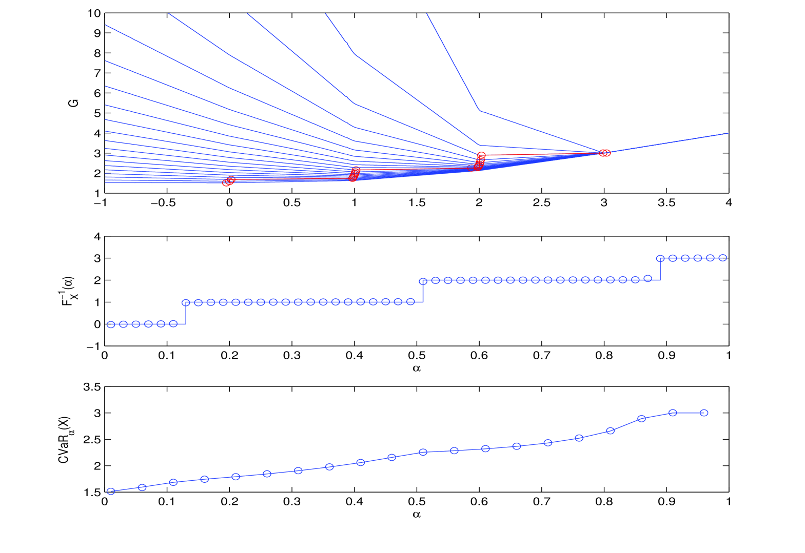
In both the algorithms, the expectations required to compute VaR and CVaR must be evaluated for different values of a parameter , namely and . This can be efficiently done by means of the Fourier transform technique. Before recalling the basic properties of this class of computational methods, we now briefly introduce a simple loss model which will be used to test the computational procedures in the final Section.
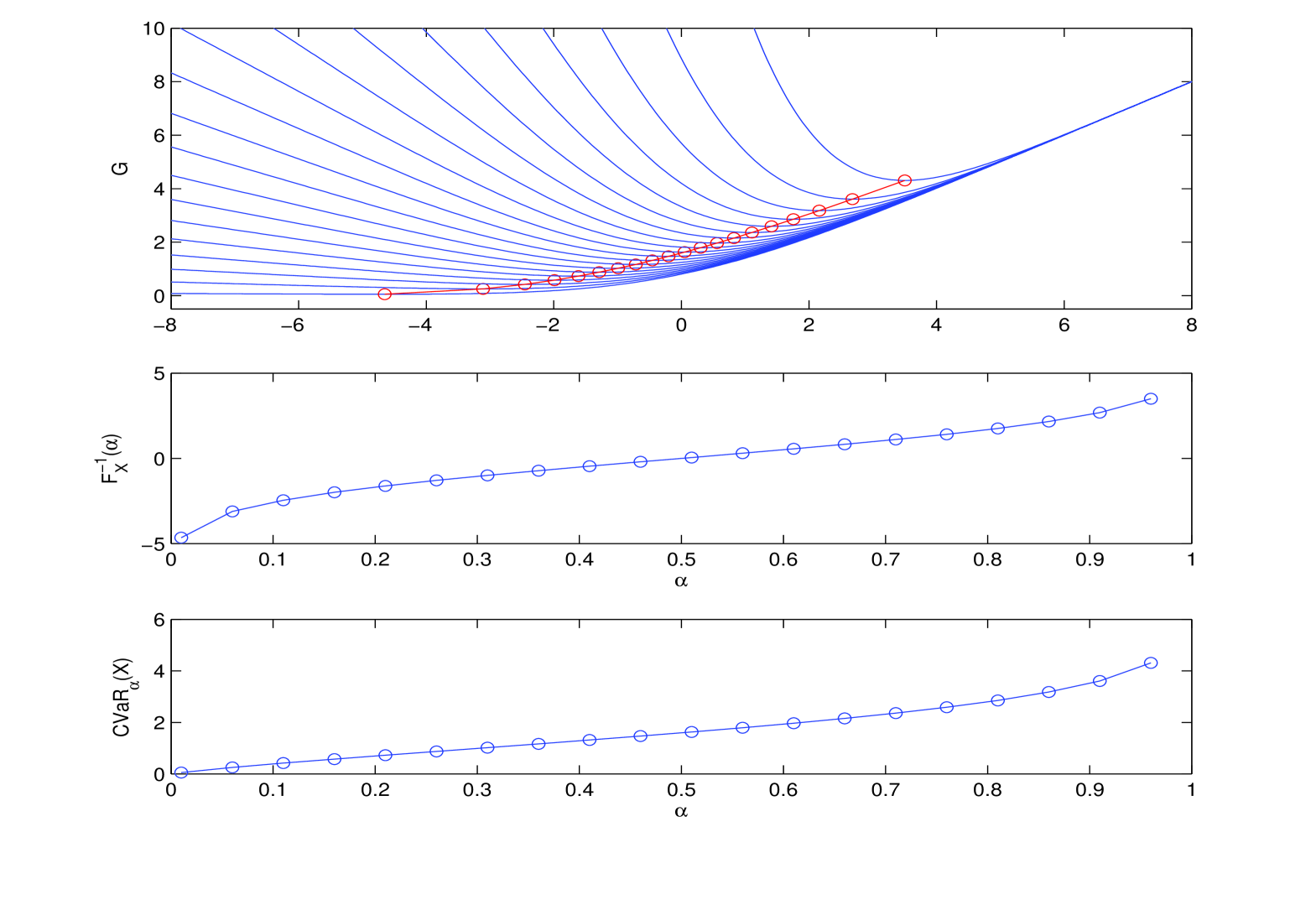
An Univariate Loss Model.
Let us consider on a filtered probability space a stochastic process of the form , , modeling the value of a risky position for . The random variable we consider is
where is the risk-free interest rate, that we can assume as a deterministic constant in the reference period for easiness of notation. In such a case the function becomes
| (5) | |||||
where . Theorem (2.1) still applies, with the constraint .
Example 2.1.
Let us consider the classical log-normal model, where , being the Wiener process, and two given parameters. In such a case, standard calculations yield
and
where is the standard normal cumulative distribution function and is the corresponding -quantile (or critical value). Finally,
3 The Fourier transform method
Fourier transform methods are efficient techniques emerged in recent years in the financial practice as one of the main methodology for the evaluation of derivatives. In fact, the no-arbitrage price of an European style contingent claim can be represented as the (conditional) expectation of the derivative payoff under a proper risk-neutral measure (see e.g. [3]). These methods essentially consist on the representation of such an expectation as the convolution of two Fourier transforms. Since the value of most derivatives depends on a trigger parameter, two main variants have been developed depending on which variable of the payoff is transformed into the Fourier space. In our setting, due to the functional (exponential) form of the transformed functions we consider, the formulas we get by applying the two approaches are essentially the same: we can pass from one to the other by simply changing the integration contour (see [21]). In the following we choose to work with the generalized Fourier transform (GFT) w.r.t. the trigger parameter . In essence, given a function , the quantity that we want to compute is , where the expectation is taken over a given probability measure . Let us consider the GFT with respect to : formally we have for
where we have defined
Notice that corresponds to the classical Fourier transform of the -damped expectation, as introduced in [5]: Fourier inversion gives
for in some strip of . The previous equalities must be justified under the appropriate conditions on the function , its transform and the characteristic function of the underlying random variables (see e.g. [18] for a thorough discussion on the subject). For our application we consider the following functions:
The reason for considering an exponential transformation of the basic risk factor is the fact that many financial models are usually introduced in the form , as in Example (2.1). Their GFT are readily obtained by means of standard (complex) integration: we summarize such results in the following
Proposition 3.1.
Let , then
| (6) |
| (7) |
| (8) |
| (9) |
Let be the (generalized) characteristic function of the r.v. . The following result can be proved as in [18].
Theorem 3.1.
(a) If , , then
| (10) |
(b) Let . If , , then
| (11) |
(c) If , , then
| (12) |
(d) If , , then
| (13) |
Remark 3.1.
It is worth noting that formula (11) is a slight generalizations of the well-known Levy’s Inversion (and Gil-Pelaez) formulas, that can be obtained by using the Residue Theorem. Furthermore, in the framework of the univariate loss model discussed in Example (2.1), we clearly have , where for , and we notice that the probability of the events has the same integral representation as (11).
Under the hypothesis of Theorem (2.1) we finally obtain an integral representation for the function :
| (14) | |||||
or, in the case of exponential models,
| (15) |
As it is widely known, the transform method deserves for an efficient evaluation of expectations by means of the FFT algorithm for a proper range of the trigger parameter. Actually, if only one value has to be evaluated for a fixed parameter or , there is no need to use FFT and a proper quadrature algorithm suffices to compute the required expectations.
Fast Fourier Transform - FFT.
This technique involves two steps:
-
•
a numerical quadrature scheme to approximate through a -point sum the integral
By using an equi-spaced grid of the line with spacing , we have
where are the integration weights222Different spacing rules can be implemented, e.g. the midpoint rule.;
-
•
given a grid , , denoted by , the sum is written as a discrete Fourier transform (DFT) when
(16) that is
where
(17)
The integral is therefore approximated over the grid as that can be efficiently computed by means of the Fast Fourier Transform algorithm, . The required values are computed with O operations. A thorough discussion on sampling and truncation errors is found in [18].
Fractional Fourier Transform - FRFT.
The condition imposes that if we refine the integration grid ( small), the range for the variable becomes larger, thus including values which cannot be useful in our valuation procedure. Fractional Fourier transform permits on the contrary to decouple the two steps: it is therefore possible to choose properly the integration range and the -spacing grid. The resulting algorithm, introduced in the financial literature in [8], involves the use of standard FFT: in terms of the number of elementary operations, the computational cost of a FRFT procedure with -point, -FRFT, is about the same as a -FFT. The advantage of running a FRFT with smaller is that it may achieve the same accuracy than a FFT with much larger .
The -th component of the -fractional discrete Fourier transform of the vector is defined as
with . The algorithm works as follows: firstly define two -point vectors
The -th component of is then computed as
where FFT-1 is the inverse fast Fourier transform and is the component-wise vector multiplication. As before, the integral can be approximated over the grid by means of the Fractional Fourier Transform algorithm,
4 Implementation and results
The numerical procedures outlined in Section 2 for the computation of VaR and CVaR both require to evaluate the distribution function and/or the stop-loss expectation of the random variable . Algorithm 1 firstly calls for a zero-finding routine that needs to compute (a sequence of) values of and then must be evaluated. Algorithm 2 must solve iteratively a univariate minimization problem requiring at each step to compute an expectation. Efficient numerical quadratures for computing Fourier integrals suffice for implementing the two algorithms without the need of calling for fast Fourier transforms. Error bounds on the approximation obtained clearly depends on the computational methods chosen for numerical integration, zero-finding and minimization routines. A third algorithm can be outlined, providing a quick-and-dirty solution, based on FFT/FRFT. Since we want to minimize w.r.t. the functions or we can approximate them for a whole range of values by applying once FFT/FRFT: from the integral representation (14) and (15), we get
and
where is the vector defined in (17), evaluated according to the functions in (14) or (15). Hence, the minimum and the corresponding minimizer of the vector will provide approximated values for CVaR and VaR, respectively.
Algorithm 3. - FFT/FRFT 1. Compute the vector through FFT/FRFT algorithm for a proper grid ; 2. Find the minimum and the corresponding minimizer of
| VaR Abs Err | CVaR Abs Err | Relative Time | |
|---|---|---|---|
| Alg 1 | |||
| Alg 2 | |||
| -FFT | |||
| -FRFT |
| , | VaR Abs Err | CVaR Abs Err | Relative Time |
|---|---|---|---|
| Alg 2 | |||
| -FFT | |||
| -FRFT |
4.1 Numerical results
In this section we firstly report some results obtained by applying the computational procedures outlined above, that is Algorithm 1,2 and 3. We considered a gaussian and a binomial random variables for Table 1, and the univariate loss model framework of Example (2.1) for Table 2: due to the analytical form of the function to be minimized (5), we applied integral representation w.r.t. the scaled variable . Pros and cons of each algorithm are easily outlined: precision and speed depend of course on the algorithms implemented, the programming language and on the computer available. In our experiment we used MatLab R2012a on a Intel Core i5 CPU with GHz. The basic steps of the algorithms (quadrature, univariate minimization, zero-finding and FFT) are those available as MatLab build-in functions.
| , , | VaR Abs Err | CVaR Abs Err | Relative Time |
|---|---|---|---|
| Alg 1 | |||
| Alg 2 | |||
| -FFT | |||
| -FRFT |
| , , | VaR Abs Err | CVaR Abs Err | Relative Time |
|---|---|---|---|
| Alg 1 | |||
| Alg 2 | |||
| -FFT | |||
| -FRFT |
In the second set of experiments, we show the effectiveness of the considered computational procedures in the univariate loss model by assuming different dynamics for and evaluating the impact of the relevant parameters on the computation of VaR and CVaR. The instances we consider are Lévy models with finite activity (Merton Jump-Diffusion) and infinite activity (Variance Gamma), and stochastic volatility models (Heston model) with jumps (Regime Switching Jump-Diffusion). But our procedure applies to all models characterized by having a computable (generalized) characteristic function. In such a cases, we used a hybrid approach consisting in two steps:
-
1.
FRFT approximation for finding a feasible starting point
-
2.
refinement of the previous estimate by starting from a local minimization routine.
In the following we simply report the GCF of the considered dynamics. Details can be found e.g. in [6].
Merton Jump-Diffusion model.
We consider a jump-diffusion setting in which the jump process is described as a marked point process (MPP). Let , and be given functions, being the measurable mark space. Without loss of generality, we can assume in the following . In the given interval , we consider therefore the dynamic
| (18) |
where is a standard brownian motion and is a MPP characterized by the intensity
Here represents the intensity of the Poisson process , while is a probability measures on which specifies the jump variable . We assume that and are independent and that is finite. The function represents the jump amplitude relative to the mark : without loss of generality, we set in the following. The GCF for is then given by
where . In the numerical example, we consider jumps characterized by a Normal distribution, so that
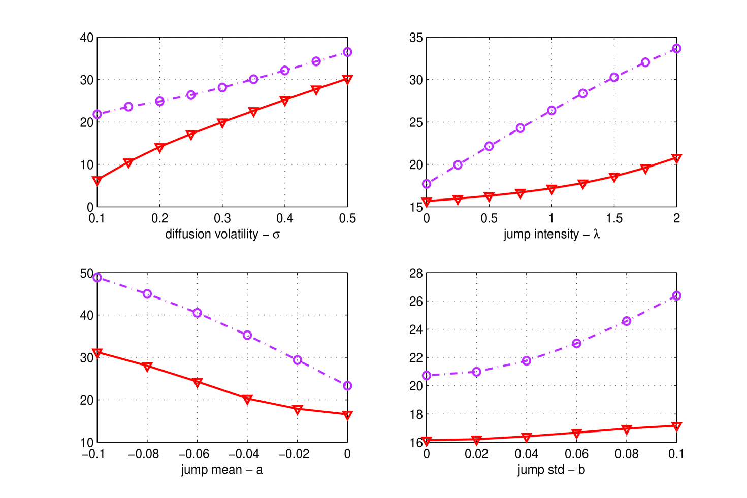
VaR and CVaR obtained by varying the diffusion volatility , the jump intensity and the jump parameters and are reported in Fig. (3).
VG model.
The Variance Gamma model was introduced in [19] and represents one of the simpler example of infinite activity Lèvy model for describing an asset value dynamic. It can be defined as a Brownian motion with drift, where time is changed by an independent gamma process with mean rate unity and variance rate , :
It has three parameters , , and the characteristic function is given by
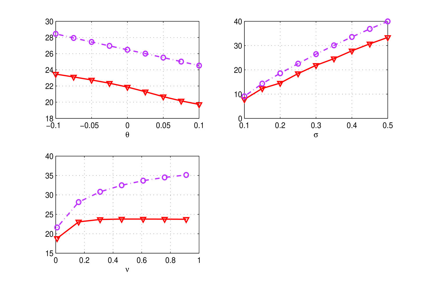
In Fig. (4) the behavior of VaR and CVaR are compared for different values of the parameters.
Regime-Switching Jump-Diffusion model.
We consider a jump-diffusion model the parameters of which are driven by a finite state and continuous time Markov chain. To be definite, let be a continuous time, homogeneous and stationary Markov chain on the state space with a generator : the elements of the matrix are positive numbers such that , for . The jump-diffusion dynamic is then modified as
| (19) |
where is a MPP characterized by the regime-switching intensity , being a set of probability measures on , one for each state (regime) . The function represents the jump amplitude relative to the mark in regime . We assume that the processes and are independent, and are conditionally independent given and that is finite for each regime .
Proposition 4.1.
Let be the generalized Fourier transform of the jump magnitude under the historical measure. Then, by letting
| (20) |
and , we have
| (21) |
where , and is the transpose of .
Simple linear constraints on the full parameter set of RSJD dynamic (19) permit to specify different models: from a regime-switching without jumps (the Naik model [20] - RSGBM) to a unique regime jump-diffusion model (JDM), which includes the standard geometrical Brownian motion (GBM).
The evaluation of the characteristic function requires to compute matrix exponentials for which efficient numerical techniques are available ([13]); conversely, the case can be considered explicitly. The following can be proved (see [21] and the references therein).
Proposition 4.2.
Let be the solutions of the quadratic equation and
Then
and therefore
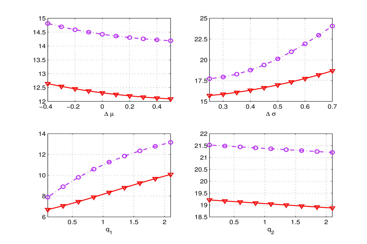
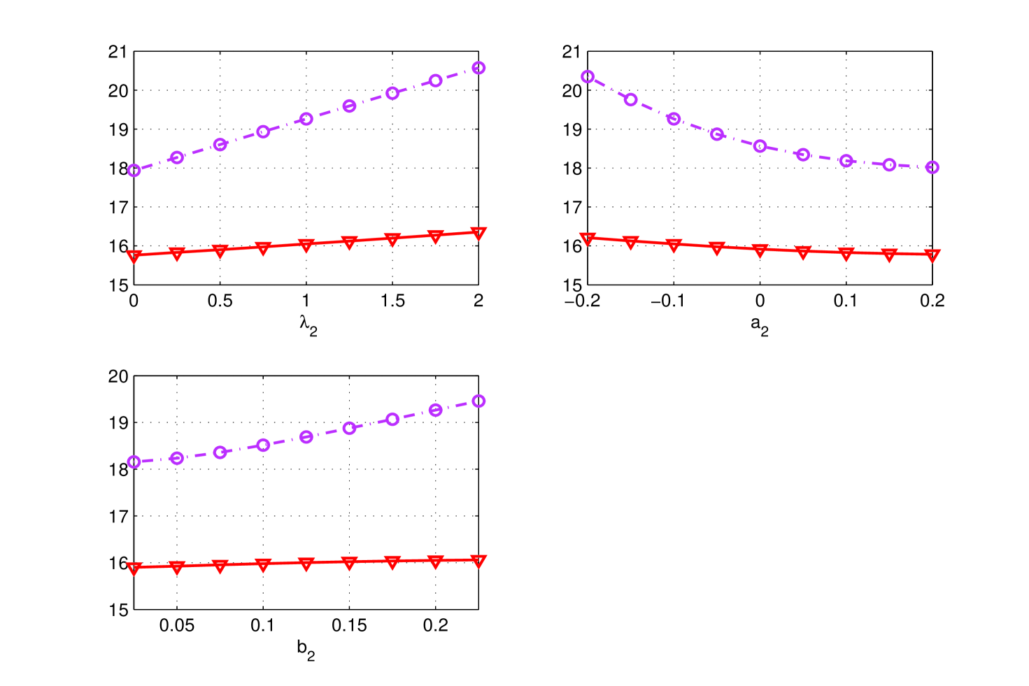
Numerical tests are reported in Figs (5), (6) for a two-state model. In order to single out the effects of the switching parameters, we firstly consider the RSGMB model, thus discarding the jump component () - Fig (5); then we fix the diffusive dynamic (, ) and vary the jump parameters according to the switching model - Fig (6).
Heston Stochastic volatility model.
Heston model [12] is certainly one of the most famous stochastic volatility dynamic for an asset price: it is defined as
| (22) | |||||
| (23) |
where , is the rate of return and , the volatility process, satisfies a CIR mean reverting dynamic with parameters (the mean reversion speed), (the long term volatility) and (the vol-vol). Furthermore, the two process are -correlated, with . The Feller condition ensures the strict positivity of . The (generalized) characteristic function of the log-price is
where
and
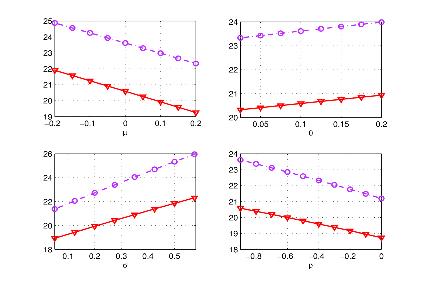
For the numerical implementation, we used the procedure outlined in [15]. The corresponding results are plotted in Fig. (7).
5 Conclusions
In this paper we consider the problem of efficiently computing CVaR and VaR of an arbitrary loss function, characterized by having a computable generalized characteristic function. We compare different numerical procedures to compute the risk measures based on the integral representation of the distribution function and the stop/loss expectation of the target loss random variable. In particular we exploit the characterization of CVaR and VaR as solution of an univariate minimization problem, as obtained by Rockafellar and Uryasev in [23]. The function to be minimized admits an integral representation as an inverse Fourier transform, under some hypothesis on the finiteness of the exponential moments of the loss distribution. Fast and reliable numerical procedures can be designed to compute the quantities of interest based on the fast Fourier transform algorithm. We finally notice that the basic characterization by Rockafellar and Uryasev is more general, since decision variables can be considered in the minimization problem: our procedure can therefore be included as part of more general optimization problem, like portfolio risk management, where the computation of VaR and CVaR plays a central role as objective functionals and/or constraints to be satisfied.
References
- [1] C. Acerbi and D. Tasche (2002), On the coherence of expected shortfall, Journal of Banking and Finance, vol. 26, pp. 1487 - 1503.
- [2] P. Artzner, F. Delbaen, J. Eber, and D. Heath, (1999). Coherent Measures of Risk, Mathematical Finance, 9(3), pp. 203-228.
- [3] T. Bjork, (2004). Arbitrage theory in continuous time, Oxford University Press, USA.
- [4] G. Bormetti, V. Cazzola, G. Livan, G. Montagna and O. Nicrosini (2010), A generalized Fourier transform approach to risk measures, Journal of Statistical Mechanics: Theory and Experiments, P01005, Online at stacks.iop.org/JSTAT/2010/P01005.
- [5] P. Carr and D. B. Madan (1999), Option valuation using the Fast Fourier Transform, Journal of Computational Finance, 2 pp. 61–73.
- [6] R. Cont and P. Tankov, Financial modelling with Jump Processes, Chapman & Hall, CRC Press, (2003).
- [7] K. Chourdakis (2004), Non-Affine option pricing, The Journal of derivatives, pp. 10-25.
- [8] K. Chourdakis (2005), Option pricing using fractional FFT, Journal of Computational Finance 8(2), pp. 1-18.
- [9] D. Duffie and J. Pan (2001), Analytical Value-at-Risk with jumps and credit risk, Finance and Stochastics, vol. 5 (2), pp. 155-180.
- [10] D. Dufresne, J. Garrido and M. Morales (2009), Fourier inversion formulas in option pricing and insurance,Methodology and Computing in Applied Probabability, 11 359–383.
- [11] H. Föllmer and A. Schied (2011), Stochastic Finance: An Introduction in Discrete Time, Walter deGruyter, Berlin.
- [12] S. Heston (1993), Closed-Form Solution for Options with Stochastic Volatility with Applications to Bond and Currency Options”, Rev. Fin. Studies, vol. 6, pp. 327-343.
- [13] N. J. Higham (2009), The scaling and Squaring Method for the Matrix Exponential Revisited, SIAM Review, 51, pp. 747–764.
- [14] W. Hürlimann (2002) Conditional value-at-risk bounds for compound Poisson risks and a normal approximation, Journal of Applied Mathematics, 3(3), pp. 141 - 154.
- [15] C. Kahl and P.Jäckel (2005), Not-so-complex logarithms in the Heston model, Wilmott, September 2005, pp. 94-103.
- [16] Y. S. Kim, S. T. Rachev, M. L. Bianchi, and F. J. Fabozzi (2010), Computing VaR and AVaR In Infinitely Divisible Distributions, Probability and Mathematical Statistics, 30 (2), 223-245.
- [17] O. Le Courtois and C. P. Walter, (2009), A Study on Value-at-Risk and Lévy Processes, available at SSRN: http://ssrn.com/abstract=1598360 or http://dx.doi.org/10.2139/ssrn.1598360.
- [18] R. W. Lee (2004), Option pricing by transform methods: extensions, unifications and error control, Journal of Computational Finance, 7, pp. 51–86.
- [19] D. B. Madan and E. Seneta (1990). The variance gamma (VG) model for share market retums. Journal of Business, 63:511-24.
- [20] V. Naik (1993), Option valuation and hedging strategies with jumps in the volatility of asset returns, Journal of Finance 48, pp. 1969-1984.
- [21] A. Ramponi (2012), On Fourier Transform Methods for Regime-Switching Jump-Diffusions and the pricing of Forward Starting Options, International Journal of Theoretical and Appplied Finance, Vol. 15, n.05.
- [22] R. T. Rockafellar and S. Uryasev (2000), Optimization of conditional value-at-risk, The Journal of Risk, 2, no. 3, pp. 21 - 41.
- [23] R. T. Rockafellar, S. Uryasev (2002), Conditional value-at-risk for general loss distributions, Journal of Banking and Finance 26, pp. 1443 - 1471.
- [24] M. Scherer, S. T. Rachev, Y. S. Kim, F. J. Fabozzi (2009), A FFT-based approximation of tempered stable and tempered infinitely divisible distributions. Preprint.