On backward smoothing algorithms
Abstract.
In the context of state-space models, skeleton-based smoothing algorithms rely on a backward sampling step which by default has a complexity (where is the number of particles). Existing improvements in the literature are unsatisfactory: a popular rejection sampling– based approach, as we shall show, might lead to badly behaved execution time; another rejection sampler with stopping lacks complexity analysis; yet another MCMC-inspired algorithm comes with no stability guarantee. We provide several results that close these gaps. In particular, we prove a novel non-asymptotic stability theorem, thus enabling smoothing with truly linear complexity and adequate theoretical justification. We propose a general framework which unites most skeleton-based smoothing algorithms in the literature and allows to simultaneously prove their convergence and stability, both in online and offline contexts. Furthermore, we derive, as a special case of that framework, a new coupling-based smoothing algorithm applicable to models with intractable transition densities. We elaborate practical recommendations and confirm those with numerical experiments.
1. Introduction
1.1. Background
A state-space model is composed of an unobserved Markov process and observed data . Given , the data are independent and generated through some specified emission distribution . These models have wide-ranging applications (e.g. in biology, economics and engineering). Two important inference tasks related to state-space models are filtering (computing the distribution of given ) and smoothing (computing the distribution of the whole trajectory , again given all data until time ). Filtering is usually carried out through a particle filter, that is, a sequential Monte Carlo algorithm that propagates weighted particles (realisations) through Markov and importance sampling steps; see Chopin and Papaspiliopoulos, (2020) for a general introduction to state-space models (Chapter 2) and particle filters (Chapter 10).
This paper is concerned with skeleton-based smoothing algorithms, i.e. algorithms that approximate the smoothing distributions with empirical distributions based on the output of a particle filter (i.e. the locations and weights of the particles at each time step). A simple example is genealogy tracking (empirically proposed in Kitagawa,, 1996 and theoretically analysed in Del Moral and Miclo,, 2001) which keeps track of the ancestry (past states) of each particles. This smoother suffers from degeneracy: for large enough, all the particles have the same ancestor at time .
The forward filtering backward smoothing (FFBS) algorithm (Godsill et al.,, 2004) has been proposed as a solution to this problem. Starting from the filtering approximation at time , the algorithm samples successively particles at times , , etc. using backward kernels. Its theoretical properties, in particular the stability as , have been studied by Del Moral et al., (2010); Douc et al., (2011).
In many applications, one is mainly interested in approximating smoothing expectations of additive functions of the form
for some functions . Such expectations can be approximated in an online fashion by a procedure described in Del Moral et al., (2010). Inspired by this, the particle-based, rapid incremental smoother (PaRIS) algorithm of Olsson and Westerborn, (2017) replaces some of the calculations with an additional layer of Monte Carlo approximation.
The backward sampling operation is central to both the FFBS and the PaRIS algorithms. The naive implementation has an cost. There have been numerous attempts at alleviating this problem in the literature, but, to our knowledge, they all lack formal support in terms of either computation complexity or stability as .
In the following five paragraphs, we elaborate on this limitation for each of the three major contenders, and we point out two related challenges with current backward sampling algorithms that we try to resolve in this article.
1.2. State of the art
First, Douc et al., (2011) proposed to use rejection sampling for the generation of backward indices in FFBS, and Olsson and Westerborn, (2017) extended this technique to PaRIS. If the model has upper-and-lower bounded transition densities, this sampler has an expected execution time (Douc et al., 2011, Proposition 2 and Olsson and Westerborn, 2017, Theorem 10). Unfortunately, most practical state space models (including linear Gaussian ones) violate this assumption, and the behaviour of the algorithm in this case is unclear. Empirically, it has been observed (Taghavi et al., 2013; Bunch and Godsill, 2013; Olsson and Westerborn, 2017, Section 4.3) that in real examples, FFBS-reject and PaRIS-reject frequently suffer from low acceptance rates, in contrary to what users would expect from an algorithm with linear complexity. To cite Bunch and Godsill, (2013), “[a]lthough theoretically elegant, the […] algorithm has been found to suffer from such high rejection rates as to render it consistently slower than direct sampling implementation on problems with more than one state dimension”. To the best of our knowledge, no theoretical result has been put forward to formalise or quantify this bad behaviour.
Second, Taghavi et al., (2013) and Olsson and Westerborn, (2017, Section 4.3) suggest putting a threshold on the number of rejection sampling trials to get more stable execution times. The thresholds are either chosen adaptively using a Kalman filter in Taghavi et al., (2013) or fixed at in Olsson and Westerborn, (2017, Section 4.3). Although improvements are empirically observed, to the best of our knowledge, no theoretical analysis of the complexity of the resulting algorithm or formal justification of the proposed threshold is available.
Third, Bunch and Godsill, (2013) use MCMC moves starting from the filtering ancestor instead of a full backward sampling step. Empirically, this algorithm seems to prevent the degeneracy associated with the genealogy tracking smoother using a very small number of MCMC steps (e.g. less than five). Unfortunately, as far as we know, this stability property is not proved anywhere in the literature, which deters the adoption of the algorithm. Using MCMC moves provides a procedure with truly linear and deterministic run time, and a stability result is the only missing piece of the puzzle to completely resolve the problem. We believe one reason for the current state of affair is that the stability proof techniques employed by Douc et al., (2011) and Olsson and Westerborn, (2017) are difficult to extend to the MCMC case.
Fourth, and this is related to the third point, the stability of the PaRIS algorithm has only been proved in the asymptotic regime. More specifically, Olsson and Westerborn, (2017) established a central limit theorem as in Corollary 5, then showed that the corresponding asymptotic error remains controlled as in Theorem 8 and Theorem 9. While non-asymptotic stability bounds for the FFBS algorithm are already available in Del Moral et al., (2010); Douc et al., (2011); Dubarry and Le Corff, (2013), we do not think that they can be extended straightforwardly to PaRIS and we are not aware of any such attempt in the literature.
Fifth, all backward samplers mentioned thus far require access to the transition density. Many models have dynamics that can be simulated from but transition densities that are not explicitly calculable. Enabling backward sampling in this scenario is challenging and will certainly require some kind of problem-specific knowledge to extract information from the transition densities, despite not being able to evaluate them exactly.
1.3. Structure and contribution
Section 2 presents a general framework which admits as particular cases a wide variety of existing algorithms (e.g. FFBS, forward-additive smoothing, PaRIS) as well as the novel ones considered later in the paper. It allows to simultaneously prove the consistency as and the stability as for all of them. The main ingredient is the discrete backward kernels, which are essentially random matrices employed differently in the offline and the online settings. On the technical side, the stability result is proved using a new technique, yielding a non-asymptotic bound that addresses the fourth point in subsection 1.2.
Next, we closely look at the use of rejection sampling and realise that in many models, the resulting execution time may be significantly heavy-tailed; see Section 3. For instance, the run time of PaRIS may have infinite expectation, whereas the run time of FFBS may have infinite variance. (Since it is technically more involved, the material for the FFBS algorithm is delegated to Supplement B.) These results address the first point in subsection 1.2 and we discuss their severe practical implications.
We then derive and analyse hybrid rejection sampling schemes (i.e. schemes that use rejection sampling only up to a certain number of attempts, and then switch to the standard method). We show that they lead to a nearly algorithm (up to some factor) in Gaussian models; again see Section 3. This stems from the subtle interaction between the tail of Gaussian densities and the finite Feynman-Kac approximation. Outside this class of model, the hybrid algorithm can still escape the complexity, although it might not reach the ideal linear run time target. These results shed some light on the second issue mentioned in subsection 1.2.
In Section 4, we look at backward kernels that are more efficient to simulate than the FFBS and the PaRIS ones. Section 4.1 describes backward kernels based on MCMC (Markov chain Monte Carlo) following Bunch and Godsill, (2013) and extends them to the online scenario. We cast this family of algorithms as a particular case of the general framework developed in Section 2, which allows convergence and stability to follow immediately. This solves the long-standing problem described in the third point of subsection 1.2.
MCMC methods require evaluation of the likelihood and thus cannot be applied to models with intractable transition densities. In Section 4.2, we show how the use of forward coupling can replace the role of backward MCMC steps in these scenarios. This makes it possible to obtain stable performance in both on-line and off-line scenarios (with intractable transition densities) and provides a possible solution to the fifth challenge describe in subsection 1.2.
Section 5 illustrates the aforementioned algorithms in both on-line and off-line uses. We highlight how hybrid and MCMC samplers lead to a more user-friendly (i.e. smaller, less random and less model-dependent) execution time than the pure rejection sampler. We also apply our smoother for intractable densities to a continuous-time diffusion process with discretization. We observe that our procedure can indeed prevent degeneracy as , provided that some care is taken to build couplings with good performance. Section 6 concludes the paper with final practical recommendations and further research directions. Table 1 gives an overview of existing and novel algorithms as well as our contributions for each.
1.4. Related work
Proposition 1 of Douc et al., (2011) states that under certain assumptions, the FFBS-reject algorithm has an asymptotic complexity. This does not contradict our results, which point out the undesirable properties of the non-asymptotic execution time. Clearly, non-asymptotic behaviours are what users really observe in practice. From a technical point of view, the proof of Douc et al., (2011, Prop. 1) is a simple application of Theorem 5 of the same paper. In contrast, non-asymptotic results such as Theorem B.1 and Theorem B.2 require more delicate finite sample analyses.
Figure 1 of Olsson and Westerborn, (2017) and the accompanying discussion provide an excellent intuition on the stability of smoothing algorithms based on the support size of the backward kernels. We formalise this support size condition for the first time by the inequality (13) and construct a novel non-asymptotic stability result based on it. In contrast, Olsson and Westerborn, (2017) depart from their initial intuition and use an entirely different technique to establish stability. Their result is asymptotic in nature.
Gloaguen et al., (2022) briefly mention the use of MCMC in PaRIS algorithm, but their algorithm is fundamentally different to and less efficient than Bunch and Godsill, (2013). Indeed, they do not start the MCMC chains at the ancestors previously obtained during the filtering step. They are thus obliged to perform a large number of MCMC iterations for decorrelation, whereas the algorithms described in our Proposition 4, built upon the ideas of Bunch and Godsill, (2013), only require a single MCMC step to guarantee stability. However, we would like to stress again that Bunch and Godsill, (2013) did not prove this important fact.
Another way to reduce the computation time is to perform the expensive backward sampling steps at certain times only. For other values of , the naive genealogy tracking smoother is used instead. This idea has been recently proposed by Mastrototaro et al., (2021), who also provided a practical recipe for deciding at which values of the backward sampling should take place and derived corresponding theoretical results.
Smoothing in models with intractable transition densities is very challenging. If these densities can be estimated accurately, the algorithms proposed by Gloaguen et al., (2022) permit to attack this problem. A case of particular interest is diffusion models, where unbiased transition density estimators are provided in Beskos et al., (2006); Fearnhead et al., (2008). More recently, Yonekura and Beskos, (2022) use a special bridge path-space construction to overcome the unavailability of transition densities when the diffusion (possibly with jumps) must be discretised.
Our smoother for intractable models are based on a general coupling principle that is not specific to diffusions. We only require users to be able to simulate their dynamics (e.g. using discretisation in the case of diffusions) and to manipulate random numbers in their simulations so that dynamics starting from two different points can meet with some probability. Our method does not directly provide an estimator for the gradient of the transition density with respect to model parameters and thus cannot be used in its current form to perform maximum likelihood estimation (MLE) in intractable models; whereas the aforementioned work have been able to do so in the case of diffusions. However, the main advantage of our approach lies in its generality beyond the diffusion case. Furthermore, modifications allowing to perform MLE are possible and might be explored in further work specifically dedicated to the parameter estimation problem.
The idea of coupling has been incorporated in the smoothing problem in a different manner by Jacob et al., (2019). There, the goal is to provide offline unbiased estimates of the expectation under the smoothing distribution. Coupling and more generally ideas based on correlated random numbers are also useful in the context of partially observed diffusions via the multilevel approach (Jasra et al.,, 2017).
In this work, we consider smoothing algorithms that are based on a unique pass of the particle filter. Offline smoothing can be done using repeated iterations of the conditional particle filter (Andrieu et al.,, 2010). Full trajectories can also be constructed in an online manner if one is willing to accept some lag approximations (Duffield and Singh,, 2022). Another approach to smoothing consists of using an additional information filter (Fearnhead et al.,, 2010), but it is limited to functions depending on one state only. Each of these algorithmic families has their own advantages and disadvantages, of which a detailed discussion is out of the scope of this article (see however Nordh and Antonsson,, 2015).
2. General structure of smoothing algorithms
In this section, we decompose each smoothing algorithm into two separate parts: the backward kernel (which determines its theoretical properties such as the convergence and the stability) and the execution mode (which is either online or offline and determines its implementation). This has two advantages: first, it induces an easy-to-navigate categorization of algorithms (see Table 1); and second, it allows to prove the convergence and the stability for each of them by verifying sufficient conditions on the backward kernel component only.
| Mode \ Kernel | FFBS kernel | PaRIS kernel | MCMC kernels | Intract. | |||||
| Offline |
|
|
(**) | ||||||
| Online | (*) Forward-additive |
|
(**) | (**) |
2.1. Notations
Measure-kernel-function notations. Let and be two measurable spaces with respective -algebras and . The following definitions involve integrals and only make sense when they are well-defined. For a measure on and a function , the notations and refer to . A kernel (resp. Markov kernel) is a mapping from to (resp. ) such that, for fixed, is a measurable function on ; and for fixed, is a measure (resp. probability measure) on . For a real-valued function defined on , let be the function . We sometimes write for the same expression. The product of the measure on and the kernel is a measure on , defined by . Other notations. • The notation is a shorthand for • We denote by the multinomial distribution supported on . The respective probabilities are . If they do not sum to , we implicitly refer to the normalised version obtained by multiplication of the weights with the appropriate constant • The symbol means convergence in probability and means convergence in distribution • The geometric distribution with parameter is supported on , has probability mass function and is noted by • Let and be two measurable spaces. Let and be two probability measures on and respectively. The o-times product measure is defined via for bounded functions . If and , we sometimes note by .
2.2. Feynman-Kac formalism and the bootstrap particle filter
Let be a sequence of measurable spaces and be a sequence of Markov kernels such that is a kernel from to . Let be an unobserved inhomogeneous Markov chain with starting distribution and Markov kernels ; i.e. for . We aim to study the distribution of given observed data . Conditioned on , the data are independent and for a certain emission distribution . Assume that there exists dominating measures not depending on such that
The distribution of is then given by
| (1) |
where and is the normalising constant. Moreover, and by convention. Equation (1) defines a Feynman-Kac model (Del Moral,, 2004). It does not require to admit a transition density, although herein we only consider models where this assumption holds. Let be a dominating measure on in the sense that there exists a function (not necessarily tractable) such that
| (2) |
A special case of the current framework are linear Gaussian state space models. They will serve as a running example for the article, and some of the results will be specifically demonstrated for models of this class. The rationale is that many real-world dynamics are partly, or close to, Gaussian. The notations for linear Gaussian models are given in Supplement A.1 and we will refer to them whenever this model class is discussed.
Particle filters are algorithms that sample from in an on-line manner. In this article, we only consider the bootstrap particle filter (Gordon et al.,, 1993) and we detail its notations in Algorithm 1. Many results in the following do apply to the auxiliary filter (Pitt and Shephard,, 1999) as well, and we shall as a rule indicate explicitly when it is not the case.
We end this subsection with the definition of two sigma-algebras that will be referred to throughout the paper. Using the notations of Algorithm 1, let
| (3) |
2.3. Backward kernels and off-line smoothing
In this subsection, we first describe three examples of backward kernels, in which we emphasise both the random measure and the random matrix viewpoints. We then formalise their use by stating a generic off-line smoothing algorithm.
Example 1 (FFBS algorithm, Godsill et al.,, 2004).
Once Algorithm 1 has been run, the FFBS procedure generates a trajectory approximating the smoothing distribution in a backward manner. More precisely, it starts by simulating index at time . Then, recursively for , given indices , it generates with probability proportional to . The smoothing trajectory is returned as . Formally, given , the indices are generated according to the distribution
where the (random) backward kernels are defined by
| (4) |
More simply, we can also look at these random kernels as random matrices of which entries are given by
| (5) |
Example 2 (Genealogy tracking, Kitagawa,, 1996; Del Moral and Miclo,, 2001).
It is well known that Algorithm 1 already gives as a by-product an approximation of the smoothing distribution. This information can be extracted from the genealogy, by first simulating index at time , then successively appending ancestors until time (i.e. setting sequentially ). The smoothed trajectory is returned as . More formally, conditioned on , we simulate the indices according to
where GT stands for “genealogy tracking” and the kernels are simply
| (6) |
Again, it may be more intuitive to view this random kernel as a random matrix, the elements of which are given by
Example 3 (MCMC backward samplers, Bunch and Godsill,, 2013).
In Example 2, the backward variable is simply set to . On the contrary, in Example 1, we need to launch a simulator for the discrete measure . Interestingly, the current value of is not taken into account in that simulator. Therefore, a natural idea to combine the two previous examples is to apply one (or several) MCMC steps to and assign the result to . The MCMC algorithm operates on the space and targets the invariant measure . If only one independent Metropolis-Hastings (MH) step is used and the proposal is , the corresponding random matrix has values
if , and
This third example shows that some elements of the matrix might be expensive to calculate. If several MCMC steps are performed, all elements of will have non-trivial expressions. Still, simulating from is easy as it amounts to running a standard MCMC algorithm. MCMC backward samples are studied in more details in Section 4.1.
We formalise how off-line smoothing can be done given random matrices ; see Algorithm 2. Note that in the above examples, our matrices are -measurable (i.e. they depend on particles and indices up to time ), but this is not necessarily the case in general (i.e. they may also depend on additional random variables, see Section 2.5). Furthermore, Algorithm 2 describes how to perform smoothing using the matrices , but does not say where they come from. At this point, it is useful to keep in mind the above three examples. In Section 2.4, we will give a general recipe for constructing valid matrices (i.e. those that give a consistent algorithm).
Algorithm 2 simulates, given and , i.i.d. index sequences , each distributed according to
Once the indices are simulated, the smoothed trajectories are returned as . Given and , they are thus conditionally i.i.d. and their conditional distribution is described by the component of the joint distribution
| (7) |
Throughout the paper, the symbol will refer to this joint distribution, while the symbol will refer to the -marginal of only. This allows the notation to make sense, where is a real-valued function defined on the hidden states.
2.4. Validity and convergence
The kernels and are both valid backward kernels to generate convergent approximation of the smoothing distribution (Del Moral,, 2004; Douc et al.,, 2011). This subsection shows that they are not the only ones and gives a sufficient condition for a backward kernel to be valid. It will prove a necessary tool to build more efficient later in the paper.
Recall that Algorithm 1 outputs particles , weights and ancestor variables . Imagine that the were discarded after filtering has been done and we wish to simulate them back. We note that, since the are given, the variables are conditionally i.i.d. We can thus simulate them back from
This is precisely the distribution of . It turns out that any other invariant kernel that can be used for simulating back the discarded will lead to a convergent algorithm as well. For instance, (Example 2) simply returns back the old , unlike which creates a new version. The kernel (Example 3) is somewhat an intermediate between the two. We formalise these intuitions in the following theorem. It is stated for the bootstrap particle filter, but as a matter of fact, the proof can be extended straightforwardly to auxiliary particle filters as well.
Assumption 1.
For all , and .
Theorem 2.1.
We use the same notations as in Algorithms 1 and 2 (in particular, denotes the transition matrix that corresponds to the considered kernel ). Assume that for any , the random matrix satisfies the following conditions:
-
•
given and , the variables for are i.i.d. and their distribution only depends on , where is the -th row of matrix ;
-
•
if is a random variable such that
, then has the same distribution as given .
A typical relation between variables defined in the statement of the theorem is illustrated by a graphical model in Figure 1. (See Bishop, 2006, Chapter 8 for the formal definition of graphical models and how to use them.) By “typical”, we mean that Theorem 2.1 technically allows for more complicated relations, but the aforementioned figure captures the most essential cases.
Theorem 2.1 is a generalisation of Douc et al., (2011, Theorem 5). Its proof thus follows the same lines (Supplement E.1). However, in our case the measure is no longer Markovian. This is because the backward kernel does not depend on alone, but also possibly on its ancestor and extra random variables. This small difference has a big consequence: compared to Douc et al., (2011, Theorem 5), Theorem 2.1 has a much broader applicability and encompasses, for instance, the MCMC-based algorithms presented in Section 4.1 and novel kernels presented in Section 4.2 for intractable densities.
As we have seen in (7), is fundamentally a discrete measure of which the support contains elements. As such, cannot be computed exactly in general and must be approximated using trajectories simulated via Algorithm 2. Theorem 2.1 is thus completed by the following corollary, which is an immediate consequence of Hoeffding inequality (Supplement E.13).
Corollary 1.
Under the same setting as Theorem 2.1, we have
2.5. Generic on-line smoother
As we have seen in Section 2.3 and Section 2.4, in general, the expectation , for a real-valued function of the hidden states, cannot be computed exactly due to the large support ( elements) of . Moreover, in certain settings we are interested in the quantities for different functions . They cannot be approximated in an on-line manner without more assumptions on the connection between and . If the family is additive, i.e. there exists functions such that
| (9) |
then we can calculate both exactly and on-line. The procedure was first described in Del Moral et al., (2010) for the kernel (i.e. the measure defined by (7) and the random kernels ), but we will use the idea for other kernels as well. In this subsection, we first explain the principle of the method, then discuss its computational complexity and the link to the PaRIS algorithm (Olsson and Westerborn,, 2017).
Principle
For simplicity, we start with the special case . Equation (7) and the matrix viewpoint of Markov kernels then give
This naturally suggests the following recursion formula to compute :
with and
| (10) |
In the general case where functions are given by (9), simple calculations (Supplement E.2) show that (10) is replaced by
| (11) |
where the matrix is defined by
and the operator extracts the diagonal of a matrix. This is exactly what is done in Algorithm 3.
Computational complexity and the PaRIS algorithm
Equations (10) and (11) involve a matrix-vector multiplication and thus require, in general, operations to be evaluated. When , Algorithm 3 becomes the on-line smoothing algorithm of Del Moral et al., (2010). The complexity can however be lowered to if the matrices are sparse. This is the idea behind the PaRIS algorithm (Olsson and Westerborn,, 2017), where the full matrix is unbiasedly estimated by a sparse matrix . More specifically, for any integer , for any , let be conditionally i.i.d. random variables simulated from . The random matrix is then defined as
and the corresponding random kernel is
| (12) |
The following straightforward proposition establishes the validity of the kernel. Together with Theorem 2.1, it can be thought of as a reformulation of the consistency of the PaRIS algorithm (Olsson and Westerborn,, 2017, Corollary 2) in the language of our framework.
Proposition 1.
The matrix has only non-zero elements out of . It is an unbiased estimate of in the sense that
Moreover, the sequence of matrices satisfies the two conditions of Theorem 2.1.
The proposition also justifies the complexity of (10) and (11), as long as is fixed as . But it is important to remark that the preceding complexity does not include the cost of generating the matrices themselves, i.e., the operations required to simulate the indices . In Olsson and Westerborn, (2017) it is argued that such simulations have an cost using the rejection sampling method whenever the transition density is both upper and lower bounded. Section 3 investigates the claim when this hypothesis is violated.
2.6. Stability
When , Algorithms 2 and 3 reduce to the genealogy tracking smoother (Kitagawa,, 1996). The matrix is indeed sparse, leading to the well-known complexity of this on-line procedure. As per Theorem 2.1, smoothing via genealogy tracking is convergent at rate if is fixed. When however, all particles will eventually share the same ancestor at time (or any fixed time ). Mathematically, this phenomenon is manifested in two ways: (a) for fixed and function , the error of estimating grows linearly with ; and (b) the error of estimating grows quadratically with . These correspond respectively to the degeneracy for the fixed marginal smoothing and the additive smoothing problems; see also the introductory section of Olsson and Westerborn, (2017) for a discussion. The random matrices are therefore said to be unstable as , which is not the case for or . This subsection gives sufficient conditions to ensure the stability of a general .
The essential point behind smoothing stability is simple: the support of or for contains more than one element, contrary to that of . This property is formalised by (13). To explain the intuitions, we use the notations of Algorithm 2 and consider the estimate
of when . The variance of the quantity above is a sum of terms. It can therefore be understood by looking at a pair of trajectories simulated using Algorithm 2.
At final time , and both follow the distribution. Under regularity conditions (e.g. no extreme weights), they are likely to be different, i.e., . This property can be propagated backward: as long as , the two variables and are also likely to be different, with however a small chance of being equal. Moreover, as long as the two trajectories have not met, they can be simulated independently given (the sigma algebra defined in (3)). In mathematical terms, under the two hypotheses of Theorem 2.1, given and , it can be proved that the two variables and are independent if (Lemma E.1, Supplement E.3).
Since there is an chance of meeting at each time step, if , it is likely that the two paths will meet at some point . When , the two indices and are both simulated according to . In the genealogy tracking algorithm, is a Dirac measure, leading to almost surely. This spreads until time , so is almost if .
Other kernels like or do not suffer from the same problem. For these, the support size of is greater than one and thus there is some real chance that . If that does happen, we are again back to the regime where the next states of the two paths can be simulated independently. Note also that the support of does not need to be large and can contain as few as elements. Even if might still be equal to with some probability, the two paths will have new chances to diverge at times , and so on. Overall, this makes quite small (Lemma E.3, Supplement E.3).
We formalise these arguments in the following theorem, whose proof (Supplement E.3) follows them very closely. The price for proof intuitiveness is that the theorem is specific to the bootstrap filter, although numerical evidence (Section 5) suggests that other filters are stable as well.
Assumption 2.
The transition densities are upper and lower bounded:
for constants .
Assumption 3.
The potential functions are upper and lower bounded:
for constants .
Remark. Since Assumption 2 implies that the ’s are compact, Assumption 1 automatically implies Assumption 3 as soon as the ’s’ are continuous functions.
Theorem 2.2.
We use the notations of Algorithms 1 and 2. Suppose that Assumptions 2 and 3 hold and the random kernels satisfy the conditions of Theorem 2.1. If, in addition, for the pair of random variables whose distribution given , and is defined by , we have
| (13) |
for some and all , ; then there exists a constant not depending on such that:
-
•
fixed marginal smoothing is stable, i.e. for and a real-valued function of the hidden state , we have
(14) -
•
additive smoothing is stable, i.e. for and the function defined in (9), we have
(15)
In particular, when is the PaRIS kernel with , Theorem 2.2 implies a novel non-asymptotic bound for the PaRIS algorithm. Olsson and Westerborn, (2017) first established a central limit theorem as and fixed, then showed that the asymptotic variance is controlled as . In contrast, we follow an original approach (whose intuition is explained at the beginning of this subsection) in order to derive a finite sample size bound.
The main technical difficulty is to prove the fast mixing of the Markov kernel product in terms of . For the original FFBS kernel, the stability proof by Douc et al., (2011) relies on the uniform Doeblin property of each of the term (page 2136, towards the end of their proof of Lemma 10) and from there, deduces the exponentially fast mixing of the product. When is approximated by a sparse matrix (which is the case for PaRIS, but also for certain MCMC-based and coupling-based smoothers that we shall see later), the aforementioned property no longer holds for each individual term . Interestingly however, the good mixing of is still conserved in the product . In Lemma E.3, we show that two trajectories generated via the latter kernel have such a small correlation that they are virtually indistinguishable from two independent trajectories generated via the former one.
Theorem 2.2 is stated under strong assumptions (similar to those used in Chopin and Papaspiliopoulos, 2020, Chapter 11.4, and slightly stronger than Douc et al., 2011, Assumption 4). On the other hand, it applies to a large class of backward kernels (rather than only FFBS), including the new ones introduced in the forthcoming sections.
In the proof of this theorem, we proceed in two steps: first, we apply existing bounds (Dubarry and Le Corff,, 2013, Theorem 3.1 and Del Moral,, 2013, Chapter 17) for the error between the -induced distribution and the true target; and second, we use our own techniques to control the error when is replaced by any other kernel satisfying (13). The term in (15) comes from the first part and we do not know whether it can be dropped. However, it does not affect the scaling of the algorithm. Indeed, with or without it, the inequality implies that in order to have a constant error in the additive smoothing problem, one only has to take (instead of without backward sampling). Moreover, from an asymptotic point of view, we always have regardless of the presence of the term, where .
3. Sampling from the FFBS Backward Kernels
Sampling from the FFBS backward kernel lies at the heart of both the FFBS algorithm (Example 1) and the PaRIS one (Section 2.5). Indeed, at time , they require generating random variables distributed according to for running from to . Since sampling from a discrete measure on elements requires operations (e.g. via CDF inversion), the total computational cost becomes . To reduce this, we start by considering the subclass of models satisfying the following assumption, which is much weaker than Assumption 2.
Assumption 4.
The transition density is strictly positive and upper bounded, i.e. there exists such that .
The motivation for the first condition will be clear after Assumption 5 is defined. For now, we see that it is possible to sample from using rejection sampling via the proposal distribution . After an -cost initialisation, new draws can be simulated from the proposal in amortised time; see Chopin and Papaspiliopoulos, (2020, Python Corner, Chapter 9), see also Douc et al., (2011, Appendix B.1) for an alternative algorithm with an cost per draw. The resulting procedure is summarised in Algorithm 4. Compared to traditional FFBS or PaRIS implementations, these rejection–based variants have a random execution time that is more difficult to analyse. Under Assumption 2, Douc et al., (2011) and Olsson and Westerborn, (2017) derive an expected complexity. However, the general picture, where the state space is not compact and only Assumption 4 holds, is less clear.
The present subsection intends to fill this gap. Our main focus is the PaRIS algorithm of which the presentation is simpler. Results for the FFBS algorithm can be found in Supplement B. We restrict ourselves to the case where , although extensions to other non compact state spaces are possible. Only the bootstrap particle filter is considered, and results from this section do not extend trivially to other filtering algorithms. In Section 5, we shall employ different types of particle filters and see that the performance could change from one type to another, which is an additional weak point of rejection-based algorithms.
Assumption 5.
The hidden state is defined on the space . The measure with respect to which the transition density is defined (cf. (2)) is the Lebesgue measure on .
This assumption together with the condition of Assumption 4 ensures that the state space model is “truly non-compact”. Indeed, if is zero whenever or , where and are respectively two compact subsets of and , then we are basically reduced to a state space model where and .
3.1. Complexity of PaRIS algorithm with pure rejection sampling
We consider the PaRIS algorithm (i.e. Algorithm 3 using the kernels). Algorithm 5 provides a concrete description of the resulting procedure, using the bootstrap particle filter. At each time , let be the number of rejection trials required to sample from . We then have
| (16) |
with defined in Assumption 4.
By exchangeability of particles, the expected cost of the PaRIS algorithm at step is proportional to , where is a fixed user-chosen parameter. Occasionally, falls into an unlikely region of and the acceptance rate becomes low. In other words, is a mixture of geometric distribution, some components of which might have a large expectation. Unfortunately, these inefficiencies add up and produce an unbounded execution time in expectation, as shown in the following proposition.
Proposition 2.
Proof.
We have
∎
In highly parallel computing architectures, each processor only handles one or a small number of particles. As such, the heavy-tailed nature of the execution time means that a few machines might prevent the whole system from moving forward. In all computing architectures, an execution time without expectation is essentially unpredictable. A common practice to estimate execution time is to run a certain algorithm with a small number of particles, then “extrapolate” to the of the definitive run. However, as is infinite for any , it is unclear what kind of information we might get from preliminary runs. In Supplement B, besides studying the execution time of rejection-based implementations of the FFBS algorithm, we will delve deeper into the difference between the non-parallel and parallel settings.
From the proof of Proposition 2, it is clear that the quantity will play a key role in the upcoming developments. We thus define it formally.
Definition 1.
The true predictive density function and its approximation are defined as
where the first equation is understood in the sense of the Radon-Nikodym derivative and the density is defined with respect to the dominating measure on (cf. (2)).
3.2. Hybrid rejection sampling
To solve the aforementioned issues of the pure rejection sampling procedure, we propose a hybrid rejection sampling scheme. The basic observation is that, for a single , direct simulation (e.g. via CDF inversion) of costs . Thus, once rejection sampling trials have been attempted, one should instead switch to a direct simulation method. In other words, it does not make sense (at least asymptotically) to switch to direct sampling after trials if or . The validity of this method is established in the following proposition, where we actually allow to depend on trials drawn so far. The proof, which is not an immediate consequence of the validity of ordinary rejection sampling, is given in Supplement E.4.
Proposition 3.
Let and be two probability densities defined on some measurable space with respect to a dominating measure . Suppose that there exists such that . Let be a sequence of i.i.d. random variables distributed according to and let be independent of that sequence. Put
and let be any stopping time with respect to the natural filtration associated with the sequence . Let be defined as if and otherwise. Then is -distributed.
Proposition 3 thus allows users to pick , where might be chosen somehow adaptively from earlier trials. In the following, we only consider the simple rule , which does not induce any loss of generality in terms of the asymptotic behaviour and is easy to implement. The resulting iteration is described in Algorithm 6.
When applied in the context of Algorithm 5, Algorithm 6 gives a smoother of expected complexity proportional to
at time , where is defined in (16)). This quantity is no longer infinite, but its growth when might depend on the model. Still, in all cases, it remains strictly larger than and strictly smaller than . Perhaps more surprisingly, in linear Gaussian models (see Supplement A.1 for detailed notations), the smoother is of near-linear complexity (up to log factors). The following two theorems formalise these claims.
Assumption 6.
The predictive density of given and the potential function are continuous functions on . The transition density is a continuous function on .
Theorem 3.1.
Theorem 3.2.
While Proposition 2 shows that has infinite expectation, Theorem 3.2 implies that its -thresholded version only displays a slowly increasing mean. To give a very rough intuition on the phenomenon, consider . Then
whereas
| (17) |
using the bound for . The main technical difficulty of the proof of Theorem 3.2 (see Supplement E.6) is to perform this kind of argument under the error induced by the finite sample size particle approximation. In the language of this oversimplified example, we want (17) to hold when does not follow any more, but only an -dependent approximation of it.
4. Efficient backward kernels
4.1. MCMC Backward Kernels
This subsection analyses and extends the MCMC backward kernel defined in Example 3. As we remarked there, the matrix is not sparse and even has some expensive-to-evaluate entries. We thus reserve it for use in the off-line smoother (Algorithm 2) whereas in the on-line scenario (Algorithm 3), we use its PaRIS-like counterpart
| (18) |
where is an independent Metropolis-Hastings chain started at , targeting the measure and using the proposal distribution . Thus, the parameter signifies that MCMC steps are applied to , and we shall use the same convention for the kernel . In both cases, the complexity of the corresponding algorithms are which is equivalent to as long as remains fixed when .
The validity and the stability of and are established in the following proposition (proved in Supplement E.9). For simplicity, only the case is examined, but as a matter of fact, the proposition remains true for .
Proposition 4.
From a theoretical viewpoint, Proposition 4 is the first result establishing the stability for the use of MCMC moves inside backward sampling. It relies on technical innovations that we have explained in Section 2.6, in particular after the statement of Theorem 2.2.
From a practical viewpoint, the advantages of independent Metropolis-Hastings MCMC kernels compared to the rejection samplers of Section 3 are the dispensability of specifying an explicit and the deterministic nature of the execution time. In practice, we observe that the MCMC smoothers are usually 10-20 times faster than the rejection sampling–based counterparts (see e.g. Figure 4) while producing essentially the same sample quality. Finally, it is not hard to imagine situations where some proposal smarter than would be beneficial. However, we only consider that one here, mainly because it already performs satisfactorily in our numerical examples.
4.2. Dealing with intractable transition densities
4.2.1. Intuition and formulation
The purpose of backward sampling is to re-generate, for each particle, a new ancestor that is different from that of the filtering step. However, backward sampling is infeasible if the transition density cannot be calculated. To get around this, we modify the particle filter so that each particle might, in some sense, have two ancestors right from the forward pass.
Consider the standard PF (Algorithm 1). Among the resampled particles , let us track two of them, say and for simplicity. The move step of Algorithm 1 will push them through using independent noises, resulting in and (that is, given and , we have and such that and are independent). Thus, for e.g. linear Gaussian models, we have . However, if the two simulations and are done with specifically correlated noises, it can happen that . The joint distribution given is called a coupling of and ; the event is called the meeting event and we say that the coupling is successful when it occurs. In that case, the particle automatically has two ancestors and at time without needing any backward sampling.
The precise formulation of the modified forward pass is detailed in Algorithm 7. It consists of building in an on-line manner the backward kernels (where ITR stands for “intractable”). The main interest of this algorithm lies in the fact that while the function may prove impossible to evaluate, it is usually possible to make and meet by correlating somehow the random numbers used in their simulations. One typical example which this article focuses on is the coupling of continuous-time processes, but it is useful to keep in mind that Algorithm 7 is conceptually more general than that.
4.2.2. Validity and stability
The consistency of Algorithm 7 follows straightforwardly from Theorem 2.1. To produce a stable routine however, some conditions must be imposed on the couplings and . We want to be different from as frequently as possible. On the contrary, we aim for a coupling of the two distributions and with high success rate so as to maximise the probability that .
Assumption 7.
There exists an such that
Assumption 8.
There exists an such that
The letters A and D in and stand for “ancestors” and “dynamics”. Assumption 8 means that the user-chosen coupling of and must be at least as times as efficient as their maximal couplings. For details on this interpretation, see Proposition 10 in the Supplement. In Lemma E.12, we also show that in spite of its appearance, Assumption 8 is actually symmetric with regards to and .
We are now ready to state the main theorem of this subsection (see Supplement E.11 for a proof).
Theorem 4.1.
The kernels generated by Algorithm 7 satisfy the hypotheses of Theorem 2.1. Thus, under Assumption 1, Algorithm 7 provides a consistent smoothing estimate. If, in addition, the Feynman-Kac model (1) satisfies Assumptions 2 and 3 and the user-chosen couplings satisfy Assumptions 7 and 8, the kernels also fulfil (13) and the smoothing estimates generated by Algorithm 7 are stable.
4.2.3. Good ancestor couplings
It is notable that Assumption 7 only considers the event , which is a pure index condition that does not take into account the underlying particles and . Indeed, if smoothing algorithms prevent degeneracy by creating multiple ancestors for a particle, we would expect that their separation (i.e. that they are far away in the state space , e.g. ) is critical to the performance. Surprisingly, it is unnecessary: two very close particles (in ) at time may have ancestors far away at time thanks to the mixing of the model.
We advise choosing an ancestor coupling such that the distance between and is small. It will then be easier to design a dynamic coupling of and with a high success rate. Furthermore, simulating the dynamic coupling with two close rather than far away starting points can also take less time when, for instance, the dynamic involves multiple intermediate steps, but the two processes couple early. One way to achieve an ancestor coupling with the aforementioned property is to first simulate , then move through an MCMC algorithm which keeps invariant and set the result to . It suffices to use a proposal looking at indices whose underlying particles are close (in ) to . Finding nearby particles are efficient if they are first sorted using the Hilbert curve, hashed using locality-sensitive hashing or put in a KD-tree (see Samet,, 2006, for a comprehensive review). In the context of particle filters, such techniques have been studied for different purposes in Gerber and Chopin, (2015), Jacob et al., (2019) and Sen et al., (2018).
4.2.4. Conditionally-correlated version
In Algorithm 7, the ancestor pairs are conditionally independent given and the same holds for the particles . These conditional independences allow easier theoretical analysis, in particular, the casting of Algorithm 7 in the framework of Theorems 2.1 and 2.2. However, they are not optimal for performance in two important ways: (a) they do not allow keeping both and when the two are not equal, and (b) the set of ancestor variables is multinomially resampled from with weights . We know that multinomial resampling is not the ideal scheme, see Supplement C.1 for discussion.
Consequently, in practice, we shall allow ourselves to break free from conditional independence. The resulting procedure is described in Algorithm 9 (Supplement C). Despite a lack of rigorous theoretical support, this is the algorithm that we will use in Section 5 since it enjoys better performance and it constitutes a fair comparison with practical implementations of the standard particle filter, which are mostly based on alternative resampling schemes.
5. Numerical experiments
5.1. Linear Gaussian state-space models
Linear Gaussian models constitute a particular class of state space models. They are characterised by Markov dynamics that are Gaussian and observations that are projection of hidden states plus some Gaussian noises. Supplement A.1 defines, for different components of these models, the notations that we shall use here. In this section, we consider an instance described in Guarniero et al., (2017), where the matrix satisfies for some . We consider the problem with and the observations are noisy versions of the hidden states with being times the identity matrix of size . Unless otherwise specified, we take and .
In this section, we focus on the performance of different online smoothers based on either genealogy tracking, pure/hybrid rejection sampling or MCMC. Rejection-based online smoothing amounts to the PaRIS algorithm, for which we use for the kernel. We take and simulate the data from the model. The benchmark additive function is simply where is the first coordinate of the vector . For a study of offline smoothers (including FFBS), see Supplement D.1. In all programs here and there, we choose and use systematic resampling for the forward particle filters (see section C.1). Regarding MCMC smoothers, we employ the kernels or consisting of only one MCMC step. All results are based on independent runs.
Although our theoretical results are only proved for the bootstrap filter, we stress throughout that some of them extend to other filters as well. Therefore, we will also consider guided particle filters in the simulations. An introduction to this topic can be found in Chopin and Papaspiliopoulos, (2020, Chapter 10.3.2), where the expression for the optimal proposal is also provided. In linear Gaussian models, this proposal is fully tractable and is the one we use.
To present efficiently the combination of two different filters (bootstrap and guided) and four different algorithms (naive genealogy tracking, pure/hybrid rejection and MCMC) we use the following abbreviations: “B” for bootstrap, “G” for guided, “N” for naive genealogy tracking, “P” for pure rejection, “H” for hybrid rejection and “M” for MCMC. For instance, the algorithm referred to as “BM” uses the bootstrap filter for the forward pass and the MCMC backward kernels to perform smoothing. Furthermore, the letter “R” will refer to the rejection kernel whenever the distinction between pure rejection and hybrid rejection is not necessary. (Recall that the two rejection methods produce estimators with the same distribution.)
Figure 2 shows the squared interquartile range for the online smoothing estimates with respect to . It verifies the rates of Theorem 2.2, although linear Gaussian models are not strongly mixing in the sense of Assumptions 2 and 3: the grid lines hint at a variance growth rate of for the MCMC and reject-based smoothers and of for the genealogy tracking ones. Unsurprisingly guided filters have better performance than bootstrap.
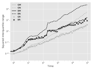
Figure 3 show box-plots of the execution time (divided by ) for different algorithms over runs. By execution time, we mean the number of Markov kernel transition density evaluations. We see that the bootstrap particle filter coupled with pure rejection sampling has a very heavy-tailed execution time. This behaviour is expected as per Proposition 2. Using the guided particle filter seems to fare better, but Figure 4 (for the same model but with ) makes it clear that this cannot be relied on either. Overall, these results highlight two fundamental problems with pure rejection sampling: the computational time has heavy tails and depends on the type of forward particle filter being used.
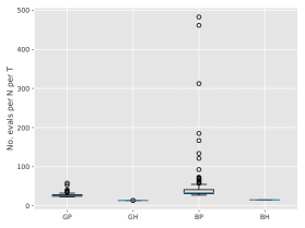
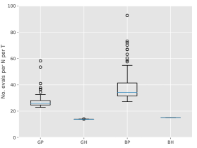
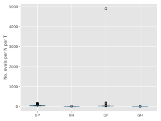
On the other hand, hybrid rejection sampling, despite having random execution time in principle, displays a very consistent number of transition density evaluations over different independent runs. Thus it is safe to say that the algorithm has a virtually deterministic execution time. The catch is that the average computational load (which is around in Figure 3) cannot be easily calculated beforehand. In any case, it is much larger than the value of MCMC smoothers (since only MCMC step is performed in the kernel ); whereas the performance (Figure 2) is comparable.
The bottom line is that MCMC smoothers should be the default option, and one MCMC step seems to be enough. If for some reason one would like to use rejection-based methods, using hybrid rejection is a must.
5.2. Lotka-Volterra SDE
Lotka-Voleterra models (originated in Lotka,, 1925 and Volterra,, 1928) describe the population fluctuation of species due to natural birth and death as well as the consumption of one species by others. The emblematic case of two species is also known as the predator-prey model. In this subsection, we study the stochastic differential equation (SDE) version that appears in Hening and Nguyen, (2018). Let represent respectively the populations of the prey and the predator at time and let us consider the dynamics
| (19) |
where with being the standard Brownian motion in and being some matrix. The parameters and are the natural birth rate of the prey and death rate of the predator. The predator interacts with (eats) the prey at rate . The quantity encodes intra-species competition in the prey population. The in its parametrisation is to line up with the Lotka Volterra jump process in where the population sizes are integers and the interaction term becomes .
The state space model is comprised of the process and its noisy observations recorded at integer times. The Markov dynamics cannot be simulated exactly, but can be approximated through (Euler) discretisation. Nevertheless, the Euler transition density remains intractable (unless the step size is exactly ). Thus, the algorithms presented in Subsection 4.2 are useful. The missing bit is a method to efficiently couple and , which we carefully describe in Supplement D.2.1.
We consider the model with , , and . The matrix is such that the covariance matrix of is . The observations are recorded on the log scale with Gaussian error of covariance matrix . The distribution of is two-dimensional normal with mean and covariance matrix . This choice is motivated by the fact that the preceding parameters give the stationary population vector . According to Hening and Nguyen, (2018), they also guarantee that neither animal goes extinct almost surely as .
By discretising (19) with time step , one can get some very rough intuition on the dynamics. For instance, per second there are about preys born. Approximately the same number die (to maintain equilibrium), of which die due to internal competition and are eaten by the predator. The duration between two recorded observations corresponds more or less to one-third generation of the prey and one-fourth generation of the predator. The standard deviation of the variation due to environmental noise is about individuals per observation period, for each animal.
Again, these intuitions are highly approximate. For readers wishing to get more familiar with the model, Supplement D.2.2 contains real plots of the states and the observations; as well as data on the performance of different smoothing algorithms for moderate values of . We now showcase the results obtained in a large scale problem where and the data is simulated from the model.
We consider the additive function . Figure 5 represents using box plots the distributions of the estimators for using either the genealogy tracking smoother (with systematic resampling; see Supplement C.1) or Algorithm 9. Our proposed smoother greatly reduces the variance, at a computational cost which is empirically to times greater than the naive method. Since we used Hilbert curve to design good ancestor couplings (see Section 4.2.3), coupling of the dynamics succeeds of the time. As discussed in the aforementioned section, starting two diffusion dynamics from nearby points make them couple earlier, which reduces the computational load afterwards.
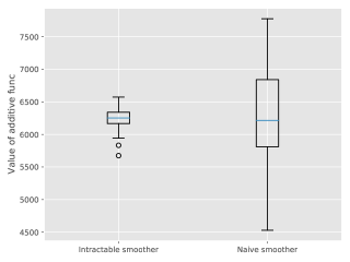
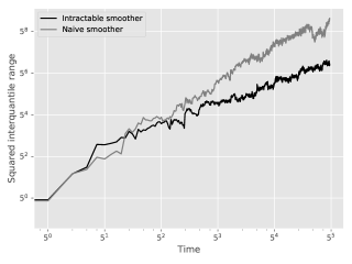
Figure 6 plots with respect to the squared interquartile range of the two methods for the estimation of . Grid lines hint at a quadratic growth for the genealogy tracking smoother (as analysed in Olsson and Westerborn,, 2017, Sect. 1) and a linear growth for the kernel (as described in Theorem 2.2).
Finally, Figure 20 (Supplement D.2.2) shows properties of the effective sample size (ESS) ratio for this model. In a nutshell, while being globally stable (between and ), it has a tendency to drift towards near from time to time due to unusual data points. At these moments, resampling kills most of the particles and aggravates the degeneracy problem for the naive smoother. As we have seen in the above figures, systematic resampling is not enough to mitigate this in the long run.
6. Conclusion
6.1. Practical recommendations
Our first recommendation does not concern the smoothing algorithm per se. It is of paramount importance that the particle filter used in in the preliminary filtering step performs reasonably well, since its output defines the support of the approximations generated by the subsequent smoothing algorithm. (Standard recommendations to obtain good performance from a particle filter are to increase , or to use better proposal distributions, or both.)
When the transition density is tractable, we recommend the MCMC smoother by default (rather than even the standard, approach). It has a deterministic, complexity, it does not require the transition density to be bounded, and it seems to perform well even with one or two MCMC steps. If one still wants to use the rejection smoother instead, it is safe to say that there is no reason not to use the hybrid method.
Although the assumptions under which we prove the stability of the smoothing estimates are strong, the general message still holds. The Markov kernel and the potential functions must make the model forget its past in some ways. Otherwise, we get an unstable model for which no smoothing methods can work. The rejection sampling – based smoothing algorithms can therefore serve as the ultimate test. Since they simulate exactly independent trajectories given the skeleton, there is no hope to perform better, unless one switches to another family of smoothing algorithms.
For intractable models, the key issue is to design couplings with high meeting probability. Fortunately, the inherent chaos of the model makes it possible to choose two very close starting points for the dynamics and thus easy to obtain a reasonable meeting probability. If further difficulties persist, there is a practical (and very heuristic) recipe to test whether one coupling of and is close to optimal. It consists in approximating and by Gaussian distributions and deduce the optimal coupling rate from their total variation distance. There is no closed formula for the total variation distance between two Gaussian distributions in high dimensions. However, it can be reliably estimated using the geometric interpretation of the total variation distance being one minus the area of the intersection created by the corresponding density graphs. In this way, one can get a very rough idea of to what extent a certain coupling realises the meeting potential that the two distributions have. If the coupling seems good and the trajectories still look degenerate, it can very well be that the model is unstable.
6.2. Further directions
The major limitation of our work is the exclusive theoretical analysis under the bootstrap particle filter. Moreover, we require that the new particles generated at step are conditionally independent given previous particles at time . This excludes practical optimisations like systematic resampling and Algorithm 9. Finally, the backward sampling step is also used in other algorithms (in particular Particle Markov Chain Monte Carlo, see Andrieu et al.,, 2010) and it would be interesting to see to what extent our techniques can be applied there.
6.3. Data and code
The code used to run numerical experiments is available at
https://github.com/hai-dang-dau/backward-samplers-code. Some of the algorithms
are already available in an experimental branch of the particles Python
package at https://github.com/nchopin/particles.
Acknowledgements
The first author acknowledges a CREST PhD scholarship via AMX funding, and wish to thank the members of his PhD defense jury (Stéphanie Allassonière, Randal Douc, Arnaud Doucet, Anthony Lee, Pierre del Moral, Christian Robert) for helpful comments on the corresponding chapter in his thesis.
We also thank Adrien Corenflos, Samuel Duffield, the associate editor, and the referees for their comments on a preliminary version of the paper.
References
- Andrieu et al., (2010) Andrieu, C., Doucet, A., and Holenstein, R. (2010). Particle Markov chain Monte Carlo methods. J. R. Stat. Soc. Ser. B Stat. Methodol., 72(3):269–342.
- Beskos et al., (2006) Beskos, A., Papaspiliopoulos, O., Roberts, G. O., and Fearnhead, P. (2006). Exact and computationally efficient likelihood-based estimation for discretely observed diffusion processes. J. R. Stat. Soc. Ser. B Stat. Methodol., 68(3):333–382. With discussions and a reply by the authors.
- Bishop, (2006) Bishop, C. M. (2006). Pattern recognition and machine learning. Information Science and Statistics. Springer, New York.
- Bou-Rabee et al., (2020) Bou-Rabee, N., Eberle, A., and Zimmer, R. (2020). Coupling and convergence for Hamiltonian Monte Carlo. The Annals of Applied Probability, 30(3):1209 – 1250.
- Bunch and Godsill, (2013) Bunch, P. and Godsill, S. (2013). Improved particle approximations to the joint smoothing distribution using Markov chain Monte Carlo. IEEE Transactions on Signal Processing, 61(4):956–963.
- Carpenter et al., (1999) Carpenter, J., Clifford, P., and Fearnhead, P. (1999). Improved particle filter for nonlinear problems. IEE Proc. Radar, Sonar Navigation, 146(1):2–7.
- Chopin, (2004) Chopin, N. (2004). Central limit theorem for sequential Monte Carlo methods and its application to Bayesian inference. Ann. Statist., 32(6):2385–2411.
- Chopin and Papaspiliopoulos, (2020) Chopin, N. and Papaspiliopoulos, O. (2020). An Introduction to Sequential Monte Carlo. Springer Series in Statistics. Springer.
- Corenflos and Särkkä, (2022) Corenflos, A. and Särkkä, S. (2022). The Coupled Rejection Sampler. arXiv preprint arXiv:2201.09585.
- Del Moral, (2004) Del Moral, P. (2004). Feynman-Kac formulae. Genealogical and interacting particle systems with applications. Probability and its Applications. Springer Verlag, New York.
- Del Moral, (2013) Del Moral, P. (2013). Mean field simulation for Monte Carlo integration, volume 126 of Monographs on Statistics and Applied Probability. CRC Press, Boca Raton, FL.
- Del Moral et al., (2010) Del Moral, P., Doucet, A., and Singh, S. S. (2010). A backward particle interpretation of Feynman-Kac formulae. M2AN Math. Model. Numer. Anal., 44(5):947–975.
- Del Moral and Miclo, (2001) Del Moral, P. and Miclo, L. (2001). Genealogies and increasing propagation of chaos for Feynman-Kac and genetic models. Ann. Appl. Probab., 11(4):1166–1198.
- Douc et al., (2005) Douc, R., Cappé, O., and Moulines, E. (2005). Comparison of resampling schemes for particle filtering. In ISPA 2005. Proceedings of the 4th International Symposium on Image and Signal Processing and Analysis, pages 64–69. IEEE.
- Douc et al., (2011) Douc, R., Garivier, A., Moulines, E., and Olsson, J. (2011). Sequential Monte Carlo smoothing for general state space hidden Markov models. Ann. Appl. Probab., 21(6):2109–2145.
- Douc et al., (2018) Douc, R., Moulines, E., Priouret, P., and Soulier, P. (2018). Markov chains. Springer Series in Operations Research and Financial Engineering. Springer, Cham.
- Dubarry and Le Corff, (2013) Dubarry, C. and Le Corff, S. (2013). Non-asymptotic deviation inequalities for smoothed additive functionals in nonlinear state-space models. Bernoulli, 19(5B):2222–2249.
- Duffield and Singh, (2022) Duffield, S. and Singh, S. S. (2022). Online particle smoothing with application to map-matching. IEEE Trans. Signal Process., 70:497–508.
- Fearnhead et al., (2008) Fearnhead, P., Papaspiliopoulos, O., and Roberts, G. O. (2008). Particle filters for partially observed diffusions. J. R. Stat. Soc. Ser. B Stat. Methodol., 70(4):755–777.
- Fearnhead et al., (2010) Fearnhead, P., Wyncoll, D., and Tawn, J. (2010). A sequential smoothing algorithm with linear computational cost. Biometrika, 97(2):447–464.
- Gerber and Chopin, (2015) Gerber, M. and Chopin, N. (2015). Sequential quasi Monte Carlo. J. R. Stat. Soc. Ser. B. Stat. Methodol., 77(3):509–579.
- Gerber et al., (2019) Gerber, M., Chopin, N., and Whiteley, N. (2019). Negative association, ordering and convergence of resampling methods. Ann. Statist., 47(4):2236–2260.
- Gloaguen et al., (2022) Gloaguen, P., Le Corff, S., and Olsson, J. (2022). A pseudo-marginal sequential Monte Carlo online smoothing algorithm. Bernoulli, 28(4):2606–2633.
- Godsill et al., (2004) Godsill, S. J., Doucet, A., and West, M. (2004). Monte Carlo smoothing for nonlinear times series. J. Amer. Statist. Assoc., 99(465):156–168.
- Gordon et al., (1993) Gordon, N. J., Salmond, D. J., and Smith, A. F. M. (1993). Novel approach to nonlinear/non-Gaussian Bayesian state estimation. IEE Proc. F, Comm., Radar, Signal Proc., 140(2):107–113.
- Guarniero et al., (2017) Guarniero, P., Johansen, A. M., and Lee, A. (2017). The iterated auxiliary particle filter. J. Amer. Statist. Assoc., 112(520):1636–1647.
- Hening and Nguyen, (2018) Hening, A. and Nguyen, D. H. (2018). Stochastic Lotka-Volterra food chains. J. Math. Biol., 77(1):135–163.
- Jacob et al., (2019) Jacob, P. E., Lindsten, F., and Schön, T. B. (2019). Smoothing with couplings of conditional particle filters. Journal of the American Statistical Association.
- Jacob et al., (2020) Jacob, P. E., O’Leary, J., and Atchadé, Y. F. (2020). Unbiased Markov chain Monte Carlo methods with couplings. J. R. Stat. Soc. Ser. B. Stat. Methodol., 82(3):543–600.
- Janson, (2011) Janson, S. (2011). Probability asymptotics: notes on notation. arXiv preprint arXiv:1108.3924.
- Jasra et al., (2017) Jasra, A., Kamatani, K., Law, K. J., and Zhou, Y. (2017). Multilevel particle filters. SIAM Journal on Numerical Analysis, 55(6):3068–3096.
- Kalman, (1960) Kalman, R. E. (1960). A new approach to linear filtering and prediction problems. Transactions of the ASME–Journal of Basic Engineering, 82(Series D):35–45.
- Kalman and Bucy, (1961) Kalman, R. E. and Bucy, R. S. (1961). New results in linear filtering and prediction theory. Trans. ASME Ser. D. J. Basic Engrg., 83:95–108.
- Kitagawa, (1996) Kitagawa, G. (1996). Monte Carlo filter and smoother for non-Gaussian nonlinear state space models. J. Comput. Graph. Statist., 5(1):1–25.
- Lévy, (1940) Lévy, P. (1940). Sur certains processus stochastiques homogènes. Compositio mathematica, 7:283–339.
- Lindvall and Rogers, (1986) Lindvall, T. and Rogers, L. C. G. (1986). Coupling of multidimensional diffusions by reflection. Ann. Probab., 14(3):860–872.
- Lotka, (1925) Lotka, A. J. (1925). Elements of physical biology. Williams & Wilkins.
- Mastrototaro et al., (2021) Mastrototaro, A., Olsson, J., and Alenlöv, J. (2021). Fast and numerically stable particle-based online additive smoothing: the adasmooth algorithm. arXiv preprint arXiv:2108.00432.
- Mörters and Peres, (2010) Mörters, P. and Peres, Y. (2010). Brownian motion, volume 30. Cambridge University Press.
- Nordh and Antonsson, (2015) Nordh, J. and Antonsson, J. (2015). A Quantitative Evaluation of Monte Carlo Smoothers. Technical report.
- Olsson and Westerborn, (2017) Olsson, J. and Westerborn, J. (2017). Efficient particle-based online smoothing in general hidden Markov models: the PaRIS algorithm. Bernoulli, 23(3):1951–1996.
- Olver et al., (2010) Olver, F. W. J., Lozier, D. W., Boisvert, R. F., and Clark, C. W., editors (2010). NIST handbook of mathematical functions. U.S. Department of Commerce, National Institute of Standards and Technology, Washington, DC; Cambridge University Press, Cambridge. With 1 CD-ROM (Windows, Macintosh and UNIX).
- Pitt and Shephard, (1999) Pitt, M. K. and Shephard, N. (1999). Filtering via simulation: auxiliary particle filters. J. Amer. Statist. Assoc., 94(446):590–599.
- Robert and Casella, (2004) Robert, C. P. and Casella, G. (2004). Monte Carlo Statistical Methods, 2nd ed. Springer-Verlag, New York.
- Roberts and Rosenthal, (2004) Roberts, G. O. and Rosenthal, J. S. (2004). General state space Markov chains and MCMC algorithms. Probab. Surv., 1:20–71.
- Samet, (2006) Samet, H. (2006). Foundations of multidimensional and metric data structures. Morgan Kaufmann.
- Sen et al., (2018) Sen, D., Thiery, A. H., and Jasra, A. (2018). On coupling particle filter trajectories. Statistics and Computing, 28(2):461–475.
- Taghavi et al., (2013) Taghavi, E., Lindsten, F., Svensson, L., and Schön, T. B. (2013). Adaptive stopping for fast particle smoothing. In 2013 IEEE International Conference on Acoustics, Speech and Signal Processing, pages 6293–6297.
- Vershynin, (2018) Vershynin, R. (2018). High-Dimensional Probability: An Introduction with Applications in Data Science. Cambridge Series in Statistical and Probabilistic Mathematics. Cambridge University Press.
- Volterra, (1928) Volterra, V. (1928). Variations and fluctuations of the number of individuals in animal species living together. ICES Journal of Marine Science, 3(1):3–51.
- Wang et al., (2021) Wang, G., O’Leary, J., and Jacob, P. (2021). Maximal couplings of the Metropolis-Hastings algorithm. In International Conference on Artificial Intelligence and Statistics, pages 1225–1233. PMLR.
- Yonekura and Beskos, (2022) Yonekura, S. and Beskos, A. (2022). Online smoothing for diffusion processes observed with noise. Journal of Computational and Graphical Statistics, 0(0):1–17.
Supplement A Additional notations
This section defines new notations that do not appear in the main text (except notations for linear Gaussian models) but are used in the Supplement.
A.1. Linear Gaussian models
Let and be two strictly positive integers and and be two full-rank matrices of sizes and respectively. Let and be two symmetric positive definite matrices of respective sizes and . A linear Gaussian state space model has the underlying Markov process defined by
where also follows a Gaussian distribution; and admits the observation process
The predictive ( given ), filtering ( given ) and smoothing ( given ) distributions are all Gaussian and their parameters can be explicitly calculated via recurrence formulas (Kalman,, 1960; Kalman and Bucy,, 1961). We shall denote their respective mean vectors and covariance matrices by , and . In particular, the starting distribution is .
A.2. Total variation distance
Let and be two probability measures on . The total variation distance between and , sometimes also denoted , is defined as . The definition remains valid if is restricted to the class of indicator functions on measurable subsets of . It implies in particular that .
Next, we state a lemma summarising basic properties of the total variation distance and defining coupling-related notions (see, e.g. Proposition 3 and formula (13) of Roberts and Rosenthal, (2004)). While the last property (covariance bound) is not in the aforementioned reference and does not seem popular in the literature, its proof is straightforward and therefore omitted.
Lemma A.1.
The total variation distance has the following properties:
-
•
(Alternative expressions.) If and admit densities and respectively with reference to a dominating measure , we have
-
•
(Coupling inequality & maximal coupling.) For any pair of random variables such that and , we have
There exist pairs for which equality holds. They are called maximal couplings of and .
-
•
(Contraction property.) Let be a Markov chain with invariant measure . Then
-
•
(Covariance bound.) For any pair of random variables such that and and real-valued functions and , we have
A.3. Cost-to-go function
A.4. The projection kernel
Let and be two measurable spaces. The projection kernel is defined by
In particular, for any function and measure defined on , we have
where the second identity shows the marginalising action of on . In the context of state space models, we define the shorthand
A.5. Other notations
For a real number , let be the largest integer not exceeding . The mapping is called the floor function • The Gamma function is defined for and is given by • Let and be two measurable spaces. Let be a (not necessarily probability) kernel from to . The norm of is defined by . In particular, for any function , we have • Let be a sequence of random variables. We say that if for any , there exists and , both depending on , such that for all . For a strictly positive deterministic sequence , we say that if . See Janson, (2011) for discussions • We use the notation to refer to the value at of the density function of the normal distribution • Let be a function from some space to another space . Let be a subset of . The restriction of to S, written , is the function from to defined by , .
Supplement B FFBS complexity for different rejection schemes
B.1. Framework and notations
The FFBS algorithm is a particular instance of Algorithm 2 where kernels are used. If backward simulation is done using pure rejection sampling (Algorithm 4), the computational cost to simulate the -th index of the -th trajectory has conditional distribution
| (21) |
At this point, it would be useful to compare this formula with (16) of the PaRIS algorithm. The difference is subtle but will drive interesting changes to the way rejection-based FFBS behaves.
If hybrid rejection sampling (Algorithm 6) is to be used instead, we are interested in the distribution of , for reasons discussed in Subsection 3.2. In a highly parallel setting, it is preferable that the distribution of individual execution times, i.e. or , are not heavy-tailed. In contrast, for non-parallel hardware, only cumulative execution times, i.e. or , matter. Even though the individual times might behave badly, the cumulative times could be much more regular thanks to effect of the central limit theorem, whenever applicable. Nevertheless, studying the finiteness of the -th order moment of is still a good way to get information about both types of execution times, since it automatically implies -th order moment (in)finiteness for both of them.
B.2. Execution time for pure rejection sampling
We show that under certain circumstances, the execution time of the pure rejection procedure has infinite expectation. Proposition 1 in Douc et al., (2011) hints that the cost per trajectory for FFBS-reject might tend to infinity when . In contrast, we show that infinite expectation might very well happen for finite sample sizes. We first give the statement for general state space models, then focus on their implications for Gaussian ones. In particular, while infinite expectations occur only under certain configurations, infinite higher moments happen in all linear Gaussian models with non-degenerate dynamics.
Theorem B.1.
Theorem B.2.
The proofs of the two assertions are given in Supplement E.7. We now look at how they are manifested in concrete examples. The first remark is that for technical reasons, Theorem B.2 gives no information on the finiteness of for (since is already greater than or equal to by definition). To study the finiteness of , we thus turn to Theorem B.1.
Example 4.
In linear Gaussian models, the integral of Theorem B.1 is equal to
where the notation refers to the density of the normal distribution. The integrand is proportional to for some quadratic form and linear form . The integral is finite if and only if is positive definite. In our case, this means that there is no non-trivial root for the equation , which is equivalent to
Put another way, is infinite whenever the intersection
contains other things than the zero vector. A common and particularly troublesome situation is when for some (but can be arbitrary) and the dimension of the states () is greater than that of the observations (). Then the above intersection remains non-trivial no matter how big is. Thus, has no expectation for any . In general, the problem is less severe as successive intersections will shrink the space quickly to . Consequently, Theorem B.1 only points out infiniteness of for close to . The bad news however will come from higher moments, as seen in the below example.
We will now focus on a simple but particularly striking example. Our purpose here is to illustrate the concepts as well as to show that their implications are relevant even in small, familiar settings. More advanced scenarios are presented in Section 5 devoted to numerical experiments.
Example 5.
We consider two one-dimensional Gaussian state-space models: they both have , , and . The only difference between them is that one has and another has . We are interested in the execution times at time (i.e. the rejection-based simulation of indices at time ). Theorem B.2 then gives for and for . The first implication is that in both cases, is a heavy-tailed random variable and therefore FFBS-reject is not a viable option in a highly parallel setting. But an interesting phenomenon happens in the sequential hardware scenario where one is rather interested in the cumulative execution time, i.e. , or equivalently, the mean number of trials per particle. In the case, non-existence of second moment prevents the cumulative regularisation effect of the central limit theorem. This is not the case for , in which the cumulative execution time actually behaves nicely (Figures 7 and 8). However, the most valuable message from this example is perhaps that the performance of FFBS-reject depends in a non-trivial (hard to predict) way on the model parameters.
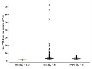
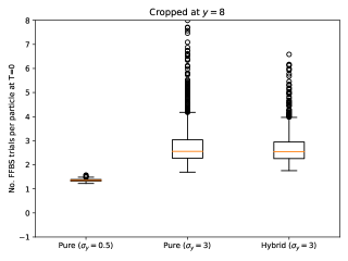
B.3. Execution time for hybrid rejection sampling
Formula (21) suggests defining the limit distribution as
where and given in Definition 1. These quantities provide the following characterisation of the cumulative execution time for the hybrid FFBS algorithm (proved in Section E.8).
Theorem B.3.
This theorem admits the following corollary for linear Gaussian models (also proved in Section E.8).
Corollary 2.
For linear Gaussian models (Supplement A.1), if smoothing is performed using the hybrid rejection version of the FFBS algorithm, the mean execution time per particle at time step is where is the dimension of .
The bound is actually quite conservative. For instance, with either or , the model considered in Example 5 admits . (Gaussian dynamics can be handled using exact analytic calculations and enables to verify the claim straightforwardly.) Theorem B.3 then gives an execution time per particle of order for hybrid FFBS, which is better than the predicted by Corollary 2. Yet another unsatisfactory point of the result is its failure to make sense of the spectacular improvement brought by hybrid rejection sampling over the ordinary procedure in the case (see Figure 7). As explained in Example 5, this is connected to the variance of and not merely the expectation; so a study of second order properties of would be desirable.
Supplement C Conditionally-correlated versions of particle algorithms
C.1. Alternative resampling schemes
In Algorithm 1, the indices are drawn conditionally i.i.d. from the multinomial distribution . They satisfy
for any . There are other ways to generate from that still verify this identity. We call them unbiased resampling schemes, and the natural one used in Algorithm 1 multinomial resampling.
The main motivation for alternative resampling schemes is performance. We refer to Chopin, (2004); Douc et al., (2005); Gerber et al., (2019) for more details, but would like to mention that the theoretical studies of particle algorithms using other resampling schemes are more complicated since are no longer i.i.d. given . We use systematic resampling (Carpenter et al.,, 1999) in our experiments. See Algorithm 8 for a succinct description and Chopin and Papaspiliopoulos, (2020, Chapter 9) for efficient implementations in running time.
C.2. Conditionally-correlated version of Algorithm 7
In this part, we present an alternative version of Algorithm 7 that does not create conditionally i.i.d. particles at each time step. The procedure is detailed in Algorithm 9. It creates on the fly backward kernels (for “intractable, conditionally correlated”). It involves a resampling step which can be done in principle using any unbiased resampling scheme. Following the intuitions of Subsection 4.2.3 and the notations of Algorithm 9, we want a scheme such that in most cases, but the Euclidean distance between and is small. Algorithm 10 proposes such a method (which we name the Adjacent Resampler). It can run in time using a suitably implemented linked list.
Supplement D Additional information on numerical experiments
D.1. Offline smoothing in linear Gaussian models
In this section, we study offline smoothing for the linear Gaussian model specified in Section 5.1. Since offline processing requires storing particles at all times in the memory, we use here instead of . Apart from that, the algorithmic and benchmark settings remain the same.
Figure 9 plots the squared interquartile range of the estimators with respect to , for different algorithms. For small , the function only looks at states close to time , whereas for bigger , recent states less affected by degeneracy are also taken into account. In all cases though, we see that MCMC and rejection-based smoothers have superior performance.
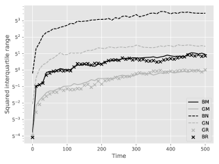
Figure 10 shows box plots of the averaged execution times (per particle per time ) based on runs. The observations are comparable to those in Section 5.1. We see a performance difference between the rejection-based smoothers using the bootstrap and the guided filters. Both have an execution time that is much more variable than hybrid rejection algorithms. The latter still need around times more CPU load than MCMC smoothers, for essentially the same precision.
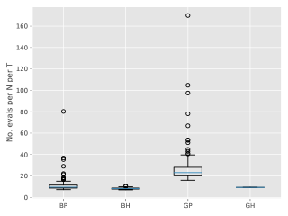
We now take a closer look at the reason behind the performance difference between the bootstrap filter and the guided one when pure rejection sampling is used. Figure 11 shows the effective sample size (ESS) of both filters as a function of time. We can see that there is an outlier in the data around time . Figure 12 box-plots the execution times divided by at for the pure rejection sampling algorithm, whereas Figures 13 and 14 do the same for and . The root of the problem is now clear: at most times there is very few difference between the execution times of the bootstrap and the guided filters. However, if an outlier is present in the data, the guided filter suddenly requires a very high number of transition density evaluation in the rejection sampler. This gives yet another reason to avoid using pure rejection sampling.

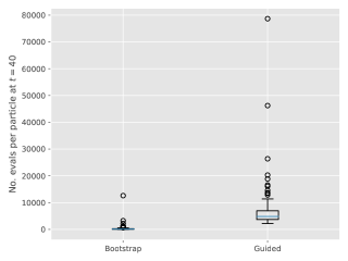
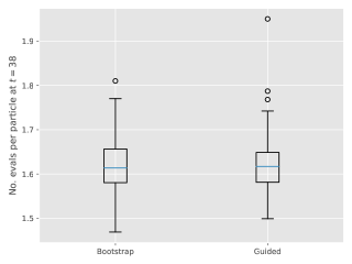
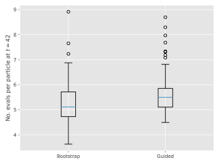
D.2. Lotka-Volterra SDE
D.2.1. Coupling of Euler discretisations
Consider the SDE
| (22) |
and two starting points and in . We wish to simulate and such that the transitions from to and to both follow the Euler-discretised version of the equation, but and are correlated in a way that increases, as much as we can, the probability that they are equal. Algorithm 11 makes it clear that it all boils down to the coupling of two Gaussian distributions.
Lindvall and Rogers, (1986) propose the following construction: if two diffusions and both follow the dynamics of (22), that is,
and the two Brownian motions are correlated via
| (23) |
where is the identity matrix and the vector is defined by
then under some regularity conditions, the two diffusions meet almost surely. (Note two special features of (23): it is valid because the term in the square bracket is an orthogonal matrix; and it ceases to be well-defined once the two trajectories have met.) Simulating the meeting time turns out to be very challenging. The Euler discretisation (Algorithm 11 + Algorithm 12) has a fixed step size , and there is zero probability that is of the form for some integer . Since the coupling transform is deterministic, the two Euler-simulated trajectories will never meet. Figure 15 depicts this difficulty in the special case of two Brownian motions in dimension (i.e. and ). Under this setting, (23) means that the two Brownian increments are symmetric with respect to the midpoint of the segment connecting their initial states. Note that the two dashed lines do cross at two points, but using them as meeting points is invalid: since they are not part of the discretisation but the result of some heuristic “linear interpolation”, it would change the distribution of the trajectories.
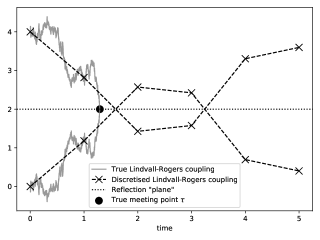
We therefore need some coupling that has a non-zero meeting probability at each -step. This can be achieved by the rejection maximal coupling (Algorithm 13, see also, e.g. Roberts and Rosenthal,, 2004) as well as the recently proposed coupled rejection sampler (Corenflos and Särkkä,, 2022). However, they all make use of rejection sampling in one way or another, which renders the execution time random. We wish to avoid this if possible. The reflection-maximal coupling (Bou-Rabee et al.,, 2020; Jacob et al.,, 2020) has deterministic cost and optimal meeting probability, but is only applicable for two Gaussian distributions of the same covariance matrix, which is not our case.
As suggested by Figure 15, the discretised Lindvall-Rogers coupling (Algorithm 12) is actually great for bringing together two faraway trajectories. Only when they start getting closer that it misses out. At that moment, the two distributions corresponding to the next -step have non-negligible overlap and would preferably be coupled in the style of Algorithm 13. We propose a modified coupling scheme that acts like Algorithm 12 when the two trajectories are at a large distance and behaves as Algorithm 13 otherwise.
The idea is to preliminarily generate a uniform draw in the “overlapping zone” of the two distributions (if they are close enough to make that easy). Next, we perform Algorithm 12 and then, any of the two simulations belonging to the overlapping zone will be replaced by the aforementioned preliminary draw (if it is available). The precise mathematical formulation is given in Algorithm 14 and the proof in Supplement E.12.
Algorithm 14 has a deterministic execution time, but it does not attain the optimal coupling rate. Yet, as , we see empirically that it still recovers the oracle coupling time defined by (23) (although we did not try to prove this formally). In Figure 16, we couple two standard Brownian motions starting from and using Algorithm 14 with different values of . It is known, by a simple application of the reflection principle (Lévy,, 1940; see also Chapter 2.2 of Mörters and Peres,, 2010), that the reflection coupling (23) succeeds after a -distributed time. We therefore have to deal with a heavy-tailed distribution and restrict ourselves to the interval . We see that the law of the meeting time is stable and convergent as . Thus, at least empirically, Algorithm 14 does not suffer from the instability problem as , contrary to a naive path space augmentation approach (see Yonekura and Beskos,, 2022 for a discussion).
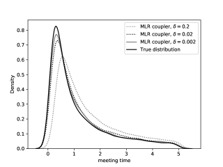
D.2.2. Supplementary figures
Figure 17 plots a realisation of the states and data with parameters given in Subsection 5.2, for a relatively small scale dataset (). While the periodic trait seen in classical deterministic Lotka-Volterra equations is still visible (with a period of around ), it is clear that here random perturbations have added considerable chaos to the system. Figures 18 and 19 show respectively the performances of the naive genealogy tracking smoother and ours (Algorithm 9) on the dataset of Figure 17. Our smoother has successfully prevented the degeneracy phenomenon, particularly for times close to . Figure 20 shows, in two different ways, the properties of effective sample sizes (ESS) in the scenario (see Section 5.2).
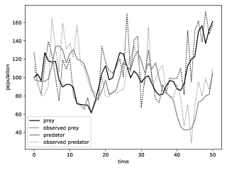
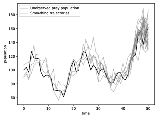
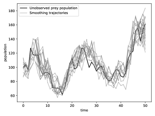
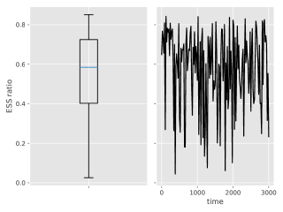
Supplement E Proofs
E.1. Proof of Theorem 2.1 (general convergence theorem)
In line with (7), we define the distribution for as the marginal of the joint distribution
| (24) |
The proof builds up on an inductive argument which links with through new innovations at time . More precisely, we have the following fundamental proposition, where is defined as the smallest -algebra containing and .
Proposition 5.
is a mixture distribution that admits the representation
| (25) |
where is defined in Algorithm 1 and is a certain probability measure satisfying
| (26) |
In other words, for any (possibly random) function such that is -measurable, we have
Moreover, , for are i.i.d. given .
The proof is postponed until the end of this subsection. This proposition gives the expression (25) for , which is easier to manipulate than (24) and which highlights, through (26), its connection to . To further simplify the notations, let us define, following Douc et al., (2011), the kernel , for , as
| (27) |
In other words, for real-valued functions , we have
The usefulness of these kernels will come from the simple remark . We also see that
which gives , where the norm of a kernel is defined in Subsection A. We are now in a position to state an importance sampling-like representation of .
Corollary 3.
Let be a (possibly random) function such that is -measurable. Suppose that is either uniformly non-negative (i.e. almost surely) or uniformly bounded (i.e. there exists a deterministic such that almost surely). Then
where is a certain random kernel such that
-
•
;
-
•
;
-
•
are i.i.d. given ;
-
•
almost surely, if is uniformly bounded and if is uniformly non-negative.
These statements are valid for under the convention and being the trivial -algebra.
Proof.
Put where is defined in Proposition 5. Then
Since is a probability measure, applying this identity twice yields
The remaining points are simple consequences of the definition of and . ∎
The corollary hints at a natural induction proof for Theorem 2.1.
Proof of Theorem 2.1.
The following calculations are valid for all , under the convention defined at the end of Corollary 3. They will prove (8) for and, at the same time, prove it for any under the hypothesis that it already holds true for . Let be a real-valued function on . Write
| (28) |
where the rewriting of is a consequence of . We will bound this difference by Hoeffding’s inequalities for ratios (see Supplement E.13 for notations, including the definition of sub-Gaussian variables that we shall use below). We have
-
•
that is -sub-Gaussian conditioned on because of Theorem E.15 (and thus unconditionally, by the law of total expectation);
-
•
and that is sub-Gaussian with parameters
if by induction hypothesis. The quantity is equal to if .
This permits to apply Lemma E.16, which results in the sub-Gaussian properties of
-
•
the quantity , with parameters , for a certain constant ;
-
•
and the quantity , which is a special case of the former one, with parameters .
Finally, we invoke Proposition 11 and deduce the sub-Gaussian property of (28) with parameters
which finishes the proof. ∎
Proof of Proposition 5.
From (24), we have
since has a term. In fact, the identity
follows directly from the backward recursive nature of Algorithm 2, and thus
| (29) |
The term is -measurable. We shall calculate the expectation of given . The following arguments are necessary for formal verification, but the result (30) is natural in light of the ancestor regeneration intuition explained in Section 2.4.
Let be a (possibly random) function such that is -measurable. Let be a random variable such that given , and , is -distributed. This automatically makes satisfy the second hypothesis of Theorem 2.1. Additionally, by virtue of its first hypothesis, the distribution of is the same given either or (see also Figure 1). We can now write
This equality means that
| (30) |
Now, put
which finishes the proof. ∎
E.2. Proof of Equation (11) (online smoothing recursion)
E.3. Proof of Theorem 2.2 (general stability theorem)
The following lemma describes the simultaneous backward construction of two trajectories and given .
Lemma E.1.
We use the same notations as in Algorithms 1 and 2. Suppose that the hypotheses of Theorem 2.1 are satisfied. Then, given , and ,
-
•
if , the two variables and are conditionally independent and their marginal distributions are respectively and ;
-
•
if , under the aforementioned conditioning, the two variables and are both marginally distributed according to . Moreover, if (13) holds, we have
(31)
In particular, the sequence of variables is a Markov chain given .
Proof.
To simplify the notations, let denote the vector . The relation between variables generated by Algorithm 2 is depicted as a graphical model in Figure 21. We consider
| (32) |
The distribution of given and is thus the -marginal of
| (33) |
which is exactly the distribution of where the ’s are defined in the statement of Theorem 2.1. By the second hypothesis of that theorem, the aforementioned distribution is equal to , which is in turn no other than . Moreover, if , (32) straightforwardly implies the conditional independence of and . When , the distribution of given and is the -marginal of
Thus, we can apply (13) for , where here plays the role of there. Equation (31) is now proved. ∎
As Lemma E.1 describes the distribution of two trajectories, it immediately gives the distribution of a single trajectory.
Corollary 4.
Under the same settings as in Lemma E.1, given , the distribution of is
Note that the corollary applies even if the backward kernel used in Algorithm 2 is not the FFBS one. This is due to the conditioning on and the second hypothesis of Theorem 2.1.
Proof of Theorem 2.2.
First of all, we remark that as per Algorithm 2, using index variables adds a level of Monte Carlo approximation to . Therefore
| (34) | ||||
where the ultimate inequality is justified by the law of total expectation and Corollary 4. (Note that are identically distributed but not necessarily independent given .) Using Lemma E.3 (stated and proved below) and putting , we have
| (35) | ||||
We now look at the first term of (34). In the fixed marginal smoothing case, for any , and any function , Douc et al., (2011) proved that
for and constants and not depending on . Using , the inequality implies
| (36) |
for . In the additive smoothing case, Dubarry and Le Corff, (2013) proved that, for ,
| (37) |
The following lemma quantifies the backward mixing property induced by Assumption 2.
Lemma E.2.
Proof.
We have
∎
Lemma E.3.
Proof.
We first handle the case . Without loss of generality, assume that , and . The covariance bound of Lemma A.1 yields
| (39) |
We shall bound this total variation distance via the coupling inequality of Lemma A.1 (Supplement A.2). The idea is to construct, in addition to and , two trajectories and i.i.d. given such that each of them is conditionally distributed according to (cf. Corollary 4). To make the coupling inequality efficient, it is desirable to make and as similar as possible (same thing for and ).
The detailed construction of the four trajectories , , and given is described in Algorithm 15. In particular, we ensure that , we have . For , if , it is guaranteed that holds . The rationale for different coupling behaviours between the times and will become clear in the proof: the former aim to control the correlation between two different trajectories and and result in the term of (38); the latter are for bounding the correlation between two times and and result in the term of the same equation.
The correctness of Algorithm 15 is asserted by Lemma E.1. Step is valid because that lemma states that the distribution of given , and is . Furthermore, we note that where
is a Markov chain given .
From (39), applying the coupling inequality of Lemma A.1 gives
| (40) |
where the last equality results from the construction of Algorithm 15. The sub-case following directly from Lemma E.4, we now focus on the sub-case . For all ,
| (41) | ||||
| by construction of Algorithm 15 | ||||
| by the law of total expectation | ||||
Thus
which, combined with (40) finishes the proof for the current sub-case . It remains to show (38) when . The proof follows the same lines as in the case , although we shall briefly outline some arguments to show how the factor disappeared. The case being trivial, suppose that and without loss of generality that . To use the coupling tools of Lemma A.1, we construct trajectories , and via Algorithm 16 and write, in the spirit of (40):
| (42) |
where the last equality follows from the construction of Algorithm 16 and the hypothesis . For all , the inequality
| (43) |
can be proved using the same techniques as those used to prove (41): applying Lemma E.2 given then invoking the law of total expectation. Repeatedly instantiating (43) gives
which, when plugged into (42), finishes the proof. ∎
Lemma E.4.
Proof.
Define , and and recall that . The sequence is a Markov chain given , but this is not necessarily the case for the sequence of Bernoulli random variables. Nevertheless, Lemma E.5 below shows that one can get bounds on two-step “transition probabilities” for , i.e. the probabilities under that given and . This motivates our following construction of actual Markov chains approximating the dynamic of . Let and be two independent Bernoulli random variables given such that
| (44) | ||||
Let and be two homogeneous Markov chains given with the same transition kernel defined by
| (45) | ||||||||
where for two events , , the notation is the ratio between and . We shall now prove by backward induction the following statement:
| (46) |
Firstly, (46) holds for and . Now suppose that it holds for some and we wish to justify it for . By Lemma E.5,
Applying the law of total expectation gives
and (46) is now proved. To finish the proof of the lemma, it is necessary to lower bound its right hand side. We start by controlling the distribution for and . We have
| (47) | ||||
and
| (48) | ||||
| by the law of total expectation | ||||
The contraction property of Lemma A.1 makes it possible to relate the intermediate distributions to the end point ones and . More specifically, (45) and Lemma A.1 lead to
| (49) |
where is the invariant distribution of a Markov chain with transition matrix , namely
| (50) |
Furthermore, an alternative expression of the total variation distance given in Lemma A.1 implies that the total variation distance between two Bernoulli distributions of parameters and is . Combining this with (49), the triangle inequality and the rough estimate , we get
where . The last inequality is straightforwardly derived by plugging respectively (50), (47) and (48) into the three terms of the preceding sum. This combined with (46) finishes the proof. ∎
Lemma E.5.
Proof.
We start by showing the following three inequalities for all and sufficiently large:
| (51) | ||||
| (52) | ||||
| (53) |
For (51), we have
| (54) |
by Lemma E.1. Next,
| (55) | ||||
Combining (54) and (55) yields (51) for large enough. To prove (52), we write
| (56) | ||||
We analyse the second term in the above expression. We have
| (57) | ||||
| by construction of Algorithm 15 | ||||
Plugging (55) and (57) into (56) yields
and thus (52) follows if is large enough. The inequality (53) is justified by combining (55), the simple decomposition and the fact that Algorithm 15 guarantees if .
We can now deduce the two inequalities in the statement of the Lemma. The first one is a straightforward double application of (53):
| by the law of total expectation | ||
Finally, we have
| using law of total expectation and the Markov property as above | ||
and the second inequality is proved. ∎
E.4. Proof of Proposition 3 (hybrid rejection validity)
Proof.
Put . Then is uniformly distributed on
The proof would be done if one could show that, given , the variable is uniformly distributed on
Note that is, by definition, the first time index where the sequence touches . Let be any subset of . We have
| (58) | ||||
By considering the special case , we see that the constant of proportionality between the first and the last terms of (58) must be , from which the proof follows. ∎
E.5. Proof of Theorem 3.1 (hybrid algorithm’s intermediate complexity)
From (16), one may have the correct intuition that as , tends in distribution to that of the variable defined as
| (59) |
where is distributed according to the predictive distribution of given and is the density of with respect to the Lebesgue measure (cf. Definition 1). The following proposition formalises the connection between and .
Proposition 6.
We have as .
Proof.
From (16) and Definition 1 one has
| (60) |
In light of (59), it suffices to establish that
| (61) |
Indeed, this would mean that for any continuous bounded function , we have
where is the geometric Markov kernel that sends each to the geometric distribution of parameter , i.e. . To this end, write
| (62) |
We study the mean squared error of the numerator:
where we have again used the exchangeability induced by step of Algorithm 5. The first term obviously tends to as by Assumptions 4 and 1. The second term also vanishes asymptotically thanks to Lemma E.6 below and Assumption 6. Assumption 1 also implies that the denominator of (62) converges in probability to some constant, via the consistency of particle approximations, see e.g. Del Moral, (2004) or Chopin and Papaspiliopoulos, (2020). Thus, by Slutsky’s theorem. Moreover, by the continuity of and the consistency of particle approximations. Using again Slutsky’s theorem yields (61). ∎
The following lemma is needed to complete the proof of Proposition 6 and is related to the propagation of chaos property, see Del Moral, (2004, Chapter 8).
Lemma E.6.
We have .
Proof.
For vectors , , and , we have, by the symmetry of the distribution of particles:
Note that
and
The dominated convergence theorem, applicable since for , finishes the proof. ∎
E.6. Proof of Theorem 3.2 (hybrid PaRIS near-linear complexity)
The following proposition shows that the real execution time for the hybrid algorithm is asymptotically at most of the same order as the “oracle” hybrid execution time.
Proposition 7.
We have
Proof.
Put
| (65) |
One can quickly verify (using the memorylessness of the geometric distribution for example) that . It will be useful to keep in mind the elementary estimate . We can now write
from which the proposition is immediate. ∎
Lemma E.7.
In addition to notations of Algorithm 1, let the function be defined as in (65) and the functions and be defined as in Definition 1. Let be a bounded non-negative deterministic function. Then, under Assumptions 1 and 4, there exist constants and depending only on the model such that
where for brevity, we shortened the integration notation (e.g. dropping , dropping from , etc.) whenever there is no ambiguity.
Proof.
We have
| (66) |
using Fubini’s theorem and the concavity of on . By a well-known result on the bias of a particle filter (which is in fact the propagation of chaos in the special case of particle), we have:
for some constant . We next show that such a bias does not change the asymptotic behavior of . More precisely,
| (67) | ||||
if is such that . In contrast, if , then provided that , we have
| (68) |
Putting together (67) and (68), we have, for ,
and so, by (66),
Again, using the result on the bias of a particle filter,
which, together with the previous inequality, implies the desired result. ∎
Proposition 8.
In linear Gaussian state space models, we have
Proof.
Let and be such that . Then
where is some constant and
We have
using the bound . The first term is of order by elementary calculus, while the second term is of order using asymptotic properties of the incomplete Gamma function, see Olver et al., (2010, Section 8.11). ∎
E.7. Proof of Theorems B.1 and B.2 (pure rejection FFBS complexity)
We start with a useful remark linking the projection kernels and the cost-to-go functions defined in Supplement A with the L-kernels formulated in (27). The proof is simple and therefore omitted.
Lemma E.8.
We have for all . Moreover, for any function , we have
Proposition 9.
We use the notations of Algorithm 2. Let be defined as in (24), where the kernels can be or any other kernels satisfying the hypotheses of Theorem 2.1. Suppose that Assumption 1 holds. Let be a (possibly random) function such that is -measurable. Then the following assertions are true:
-
(a)
Suppose that , where and are defined in Definition 1. Then
-
(b)
Suppose that . Then
Proof.
Part (a). We shall prove by induction the statement
For , it follows from part (a)’s hypothesis and Lemma E.8. Indeed,
For , we have
| by Corollary 3 and law of total expectation | |||
Part (b). Similar to part (a), we shall prove by induction the statement
Again, by Corollary 3, this quantity is equal to
and the expectation of the numerator given is , which tends to in probability by induction hypothesis. Lemma E.11 (see below at the end of the section), the classical result and Stutsky’s theorem concludes the proof. ∎
Proof of Theorem B.1.
Proof of Theorem B.2.
We use notations from Definition 1 and Supplement A.1. We note the density of the specified normal distribution at point . Using Lemma E.9, Proposition 9 and (21), we have
The theorem then follows from elementary arguments, by noting that is a mixture of Gaussian distributions with covariance matrix . ∎
Lemma E.9.
Let be a -valued random variable. Suppose is another random variable such that . Then for any real number ,
Proof.
By the definition of , we have
A natural idea is then to approximate the sum by the integral , from which one easily extracts the factor. This is however technically laborious, since the function is not monotone on the whole real line. It is only so starting from a certain which itself depends on . We would therefore rather write
with the natural interpretation of expressions when . Using as a shorthand for “ and are either both finite or both infinite”, we have
∎
The following lemma is elementary. Its proof is therefore omitted.
Lemma E.10.
Let be a -valued random variable and let and be two continuous functions from to . Suppose that and are both finite. Then is finite if and only if is so.
Lemma E.11.
Let be non-negative random variables. Suppose that there exist -algebras such that . Then .
Proof.
Fix . By Markov’s inequality, . Therefore, the bounded random variable tends to in probability, hence also in expectation. The law of total expectation then gives , which, by varying , establishes the convergence of to in probability. ∎
E.8. Proof of Theorem B.3 and Corollary 2 (hybrid FFBS complexity)
Proof of Theorem B.3.
E.9. Proof of Proposition 4 (MCMC kernel properties)
Proof.
Let be such that . Moreover, let be such that
Given , and , the kernel applies to one or more several MCMC steps keeping invariant . Since , it follows that too. On the other hand, and share the same distribution given , and . Hence they also do, given and only. This implies that , which is the same as . Thus have the same distribution as given , as required by Theorem 2.1. The arguments for the kernel are similar.
To show that a certain kernel satisfies (13), we look at two conditionally i.i.d. simulations and from and lower bound the probability that they are different. For the kernel , the variables and both result from one step of MH applied to . Let and be the corresponding MH proposals. A sufficient condition for is that and the two proposals are both accepted. The acceptance rate is at least by Assumption 2 and the probability that is
by Assumption 3. Thus (13) is satisfied for for large enough. Similarly, the probability that for the kernel with can be lower-bounded via the probability that (where and are defined in (18)). Thus using the same arguments, (13) is satisfied here for . ∎
E.10. Conditional probability of maximal couplings
In general, there exist multiple maximal couplings of two random distributions (i.e. couplings that maximise the probability of equality of the two variables). However, they all satisfy a certain conditional probability property stated in the following lemma. It is closely related to results on the coupling density on the diagonal (see e.g. Wang et al.,, 2021, Lemma 2 or Douc et al.,, 2018, Theorem 19.1.6). Its statement, which we were unable to find in the literature in the exact form we need, is obvious in the discrete case but requires lengthier arguments in the continuous one.
Proposition 10.
Let and be two random variables with densities and with respect to some dominating measure defined on a space . Then, the following inequality holds almost surely:
| (69) |
Moreover, the equality occurs almost surely if and only if and form a maximal coupling.
Proof.
The following lemma establishes the symmetry of Assumption 8. Again, its statement is obvious in the discrete case, though some work is needed to rigorously justify the continuous one.
Lemma E.12.
Let and be two random variables of densities and w.r.t. some dominating measure defined on some space . Suppose that almost-surely
for some . Then almost-surely,
Proof.
We introduce a non-negative test function and write
which implies the desired result. ∎
E.11. Proof of Theorem 4.1 (intractable kernel properties)
Proof.
Proof.
We write (and define new notations along the way):
Thus
by the boundedness of the function between and . From this, we get the desired result by virtue of Assumption 7. ∎
E.12. Validity of Algorithm 14 (modified Lindvall-Rogers coupler)
Recall that generating a random variable is equivalent to uniformly simulating under the graph of its density (see e.g. Robert and Casella,, 2004, The Fundamental Theorem of Simulation, chapter 2.3.1). Algorithm 14’s correctness is thus a direct corollary of the following intuitive lemma.
Lemma E.14.
Let and be two subsets of with finite Lebesgue measures. Let and be two not necessarily independent random variables distributed according to and respectively. Denote by the intersection of and ; and by a certain -distributed random variable that is independent from . Define and as
and
Then and .
Proof.
Given , the two variables and have the same distribution (which is ). Thus, the definition of implies that and have the same (unconditional) distribution. The same argument applies to and notwithstanding the asymmetry in the definition of . ∎
E.13. Hoeffding inequalities
This section proves a Hoeffding inequality for ratios, which helps us to bound (28). It is essentially a reformulation of Douc et al., (2011, Lemma 4) in a slightly more general manner.
Definition 2.
A real-valued random variable is called -sub-Gaussian if
This definition is close to other sub-Gaussian definitions in the literature, see e.g. Vershynin, (2018, Chapter 2.5). It basically means that the tails of decreases at least as fast as the tails of the distribution, which is itself -sub-Gaussian. The following result is classic.
Theorem E.15 (Hoeffding’s inequality).
Let be i.i.d. random variables with mean and almost surely contained between and . Then is -sub-Gaussian.
The following lemma is elementary from Definition 2. The proof is omitted.
Lemma E.16.
Let and be two (not necessarily independent) random variables. If is -sub-Gaussian and is -sub-Gaussian, then is -sub-Gaussian.
We are ready to state the main result of this section.
Proposition 11 (Hoeffding’s inequality for ratios).
Let , , , be random variables such that is -sub-Gaussian and is -sub-Gaussian. Then is sub-Gaussian with parameters where
The terms with inf-norm can be infinite if the corresponding random variables are unbounded.