On best constants in $L^{2}$ approximation

In this paper we consider the following $n$-width problem: determine the smallest constant $d_{n}$ for which there exists an $n$-dimensional subspace $X_{n}$ of $L^{2}(a,b)$ such that for all $u\in H^{r}(a,b)$, $r\geq 1$,

$$\min_{v\in X_{n}}\|u-v\|\leq d_{n}\|u^{(r)}\|.$$

(1)

This problem was originally studied in the first half of the previous century by Kolmogorov [14], who showed that $d_{n}$, for $n\geq r$, corresponds to the $(n+1)$-st eigenvalue of a certain differential operator. In fact, for $r=1$ he showed that $d_{n}=(b-a)/(n\pi)$.

The related problem of finding a subspace $X_{n}$ that achieves the smallest constant $d_{n}$ in (1), a so-called optimal subspace for $H^{r}(a,b)$, was also studied by Kolmogorov. He showed that an optimal subspace for $H^{r}(a,b)$ is the span of the first $n$ eigenfunctions of the mentioned eigenvalue problem. Further optimal subspaces were later found by Melkman and Micchelli [17] and by Floater and Sande [8]. The $n$-width problem was a major topic in the 70s and 80s [11, 12, 24, 13, 18, 17, 15, 23, 22] and there has been recent activity in the context of Isogeometric Analysis (IGA) [7, 8, 10, 9, 21, 4].

In [14] Kolmogorov further claimed that for $(a,b)=(0,1)$,

$$d_{n}=\Big{(}\frac{1}{\pi n}\Big{)}^{r}+O\Big{(}\frac{1}{n}\Big{)}^{r+1},$$

(2)

as $n\to\infty$. In [20, Chapter VII] Pinkus gives a proof that $d_{n}=O(n^{-r})$ as $n\to\infty$. As far as we know, no further asymptotic results concerning $d_{n}$ are known.

Our first result is to provide the following bounds for $d_{n}$.

Note that in the case $(a,b)=(0,1)$ this theorem gives a proof of (2).

Isogeometric Galerkin methods have been previously used to approximate $n$-widths [7]. Our tests suggest that these methods are adequate for small values of $r$ and $n$, e.g. up to $r,n\approx 5$. The second contribution in this paper is to propose a simple superconvergent collocation method that computes a good approximation of $d_{n}$ for $r$ and $n$ in the range of tens. A byproduct of the numerical method is the approximate computation of the internal knots of the first optimal spline space of Melkman and Micchelli [17]. These knots were recently used by Chan and Evans [4] in their numerical method for wave propagation based on IGA. By using the optimal knots of Melkman and Micchelli they were able to improve the approximation properties and the maximum stable timestep for their method. Numerical methods to approximate these knots are therefore highly desirable in the context of IGA.

The results of our numerical method lead us to the following conjecture:

In other words, it appears that $d_{n}^{-1/r}$ approaches the midpoint of the upper and lower bounds in Theorem 1.

First we prove the lower bound of $d_{n}$. Let

$$H^{r}_{1}=\{u\in H^{r}(a,b):u^{(k)}(a)=u^{(k)}(b)=0,\,1\leq k<r,\,k\text{ odd}\}.$$

As proved in [10, Theorem 1], the $n$-width of $H^{r}_{1}$ is $(b-a)^{r}/(\pi n)^{r}$, i.e., for each $n\geq 1$ there exists $X_{n}$ such that

$$\min_{v\in X_{n}}\|u-v\|\leq\Big{(}\frac{b-a}{\pi n}\Big{)}^{r}\|u^{(r)}\|,\qquad\forall u\in H^{r}_{1},$$

(3)

and for no $X_{n}$ the above inequality holds for with a smaller constant. Since $H^{r}_{1}$ is a subset of $H^{r}(a,b)$ we have

$$d_{n}\geq\Big{(}\frac{b-a}{\pi n}\Big{)}^{r}.$$

The upper bound for $d_{n}$ is obtained by making a specific choice of $X_{n}$. Let $S$ be the space of $C^{r-2}$ piecewise polynomials of degree $r-1$ on the uniform partition of $(a,b)$ in $m$ segments. Then for all $u\in H^{r}(a,b)$ we have by [3, Theorem 1] (or [21, Theorem 1]) that

$$\min_{v\in S}\|u-v\|\leq\Big{(}\frac{b-a}{\pi m}\Big{)}^{r}\|u^{(r)}\|.$$

(4)

Since $\dim S=m+r-1$, letting $n=\dim S\geq r$ we deduce that

$$d_{n}\leq\Big{(}\frac{b-a}{\pi(n-r+1)}\Big{)}^{r}.$$

This completes the proof of Theorem 1.

It follows from [14, 17, 20, 8] that $d_{n}^{-2}$ is equal to the $(n+1)$-th smallest eigenvalue (counting the $r$ multiplicities of zero) of the eigenvalue problem

$$\left\{\begin{aligned} &(-1)^{r}\psi^{(2r)}(x)=\mu\psi(x)&&&x\in(a,b),\\ &\psi^{(k)}(a)=\psi^{(k)}(b)=0&&&k=r,r+1,\dots,2r-1.\end{aligned}\right.$$

(5)

Moreover, the eigenfunctions corresponding to the $n$ smallest eigenvalues span an optimal space $X_{n}$. Note in particular, that $0$ is an eigenvalue of (5) with multiplicity $r$ and the null space is the space of polynomials of degree $r-1$. It is straightforward to see that in the case $r=1$ the eigenvalue problem (5) can be solved analytically, and in this case the eigenvalues are

$$0,\left(\frac{\pi}{b-a}\right)^{2},\left(\frac{2\pi}{b-a}\right)^{2},\left(\frac{3\pi}{b-a}\right)^{2}\ldots,$$

and the eigenfunctions are

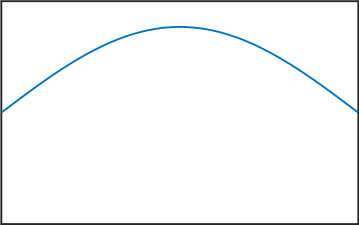
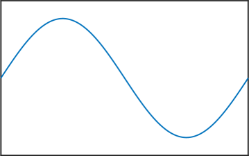
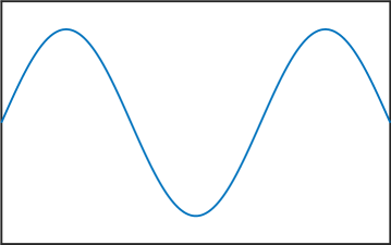
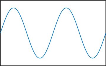
$$1,\cos\left(\pi\frac{x-a}{b-a}\right),\cos\left(2\pi\frac{x-a}{b-a}\right),\cos\left(3\pi\frac{x-a}{b-a}\right),\ldots.$$

It can further be shown that for any $r$ the eigenvalue problem in (5) has the same non-zero eigenvalues as the problem with Dirichlet boundary conditions [8]:

$$\left\{\begin{aligned} &(-1)^{r}\phi^{(2r)}(x)=\mu\phi(x)&&&x\in(a,b),\\ &\phi^{(k)}(a)=\phi^{(k)}(b)=0&&&k=0,1,\dots,r-1.\end{aligned}\right.$$

(6)

In particular, (6) has a trivial null space. Thus, for $n\geq r$, $d_{n}^{-2}$ is the $(n+1-r)$-th eigenvalue of (6). For $r=1$ the eigenvalues of (6) are

$$\left(\frac{\pi}{b-a}\right)^{2},\left(\frac{2\pi}{b-a}\right)^{2},\left(\frac{3\pi}{b-a}\right)^{2}\ldots,$$

and the eigenfunctions are

$$\sin\left(\pi\frac{x-a}{b-a}\right),\sin\left(2\pi\frac{x-a}{b-a}\right),\sin\left(3\pi\frac{x-a}{b-a}\right),\ldots.$$

Let $g$ be the Green’s function associated to (6). Since the differential operator in (6) is self-adjoint it follows that $g$ is symmetric, i.e., $g(x,y)=g(y,x)$. Moreover, it is the distributional solution of

$$\left\{\begin{aligned} &\partial^{2r}_{x}g(x,y)=(-1)^{r}\delta_{y},&&&x\in(a,b),\\ &\partial^{k}_{x}g(x,y)|_{x\in\{a,b\}}=0,&&&k=0,1,\ldots,r-1,\ y\in(a,b)\end{aligned}\right.$$

(7)

where $\delta_{y}$ is the Dirac’s delta at $y$, i.e., $\delta_{y}f=f(y)$.

For example, for $r=1$,

$$B[a,y,b](x)=\begin{cases}(x-a)/(y-a)&x\leq y,\cr(b-x)/(b-y)&x\geq y,\end{cases}$$

and so

$$g(x,y)=\begin{cases}(x-a)(b-y)/(b-a)&x\leq y,\cr(y-a)(b-x)/(b-a)&x\geq y.\end{cases}$$

For $r=2$,

$$B[a,a,y,b,b](x)=\frac{(x-a)^{2}}{(y-a)^{2}(b-a)^{2}}\big{(}(b-a)(y-x)+2(b-x)(y-a)\big{)},\quad x\leq y,$$

and so

$$g(x,y)=\frac{(x-a)^{2}(b-y)^{2}}{6(b-a)^{3}}\big{(}(b-a)(y-x)+2(b-x)(y-a)\big{)},\quad x\leq y.$$

By the symmetry of $g(x,y)$, we have

$$g(x,y)=g(y,x),\quad y\leq x.$$

For general $r$, we can evaluate $g(x,y)$ for $x\in[a,y]$ by first using the usual Cox-de Boor-Mansfield algorithm to evaluate the B-spline in (8) (after adding knots to both ends of the knot vector appropriately) and then multiplying by the scaling factor. For $x\in[y,b]$, we just set $g(x,y)=g(y,x)$.

In this section we describe a simple numerical method to approximate the eigenvalues and eigenfunctions of (6). We remind that for $r=1$ the eigenvalues and eigenfunctions are known analytically and so we only need to consider the case $r\geq 2$. Recalling that $g$ is the Green’s function to (6) we discretize the following equivalent formulation of (6)

$$\int_{a}^{b}g(x,y)\phi(y)\,dy=\lambda\phi(x),$$

(9)

where $\lambda=1/\mu$. We consider the uniform partition of $[a,b]$ in $m+1$ segments with nodes $\Xi=[\xi_{0},\dots,\xi_{m+1}]$

$$\xi_{k}=a+kh,\qquad h=(b-a)/(m+1).$$

By approximating the integral in (9) with the trapezoidal rule on each segment $[\xi_{i},\xi_{i+1}]$ and remembering $g(x,a)=g(x,b)=0$ we obtain the approximate equation

$$\lambda\phi(x)=\int_{a}^{b}g(x,y)\phi(y)\,dy\approx h\sum_{\ell=1}^{m}g(x,\xi_{\ell})\phi(\xi_{\ell}).$$

Discretizing $\phi$ with its values $\bm{v}_{\phi}$ at $\xi_{1},\dots,\xi_{m}$ we obtain the finite dimensional eigenproblem

$${\mathtt{G}}\bm{v}_{\phi}=\lambda\bm{v}_{\phi},\qquad{\mathtt{G}}:=[g(\xi_{k},\xi_{\ell})]_{k,\ell=1,\dots,m}.$$

(10)

The $k$-th eigenpair of (10) are then an approximation to the $k$-th eigenpair of (6) and (9). We remark that such approximations of the eigenvalues of integral operators have been studied before [1, 2, 5, 19]. Let $(\lambda_{k},\phi_{k})$ be the $k$-th eigenpair of (9) and $(\lambda_{k,h},\phi_{k,h})$ be the $k$-th eigenpair of (10) such that $\max_{x\in[a,b]}|\phi_{k}(x)|=\max_{x\in[a,b]}|\phi_{k,h}(x)|=1$. From [2] and [19] we then obtain the following error estimate for our eigenvalues and eigenfunctions: for all $r$ and $k$ there exists a constant $C>0$ such that for all $h<(k+1)^{-1}$ we have

	$\displaystyle|\lambda_{k}-\lambda_{k,h}|$	$\displaystyle\leq C\max_{x\in[a,b]}|E_{k}(x)|,$		(11)
	$\displaystyle\max_{x\in[a,b]}|\phi_{k}(x)-\phi_{k,h}(x)|$	$\displaystyle\leq C\max_{x\in[a,b]}|E_{k}(x)|,$

where $E_{k}(x)$ is the quadrature error of the trapezoidal rule

$$E_{k}(x):=\int_{a}^{b}f_{k}(x,y)\,dy-h\sum_{\ell=1}^{m}f_{k}(x,\xi_{\ell}),$$

and $f_{k}(x,y):=g(x,y)\phi_{k}(y)$. Since $f_{k}(x,\cdot)\in C^{2}([a,b])$ for all $r\geq 2$ we expect the error to be $O(h^{2})$ as $h\to 0$. However, for $r\geq 3$, the method is superconvergent as we prove by the following argument. The function $g(x,\cdot)\in C^{2r-2}([a,b])$ for each $x\in[a,b]$ and since the eigenfunction $\phi_{k}\in C^{\infty}([a,b])$ we have $f_{k}(x,\cdot)\in C^{2r-2}([a,b])$. Now for any $p\leq r-2$ we can use the Euler-Maclaurin expansion [6, Section 3.4.5] to obtain

	$\displaystyle E_{k}(x)=$	$\displaystyle-\sum_{j=1}^{p}\frac{B_{2j}}{(2j)!}h^{2j}(\partial_{y}^{2j-1}f_{k}(x,b)-\partial_{y}^{2j-1}f_{k}(x,a))$
		$\displaystyle-\frac{B_{2p+2}}{(2p+2)!}h^{2p+2}\partial_{y}^{2p+2}f_{k}(x,\eta_{x}),$

for some $\eta_{x}\in(a,b)$, and where $B_{j}$ is the $j$-th Bernoulli number. From the fact that $\partial_{y}^{j}g(x,y)|_{y=a,b}=\partial_{y}^{j}\phi_{k}(y)|_{y=a,b}=0$ for all $j=0,\ldots,r-1$, we deduce that $\partial_{y}^{j}f_{k}(x,y)|_{y=a,b}=0$ for all $j=0,\ldots,2r-1$. We now let $p=r-2$ and take the maximum over all the $\eta_{x}\in[a,b]$ to obtain

$$|\lambda_{k}-\lambda_{k,h}|+\max_{x\in[a,b]}|\phi_{k}(x)-\phi_{k,h}(x)|\leq Ch^{2r-2}\max_{x,y\in[a,b]}|\partial_{y}^{2r-2}f_{k}(x,y)|.$$

(12)

Recalling that $d_{n}=\lambda_{n+1-r}^{1/2}$ this implies that for some constant $C>0$, depending only on $r$ and $n$, we have

$$|d_{n}-\lambda_{n+1-r,h}^{1/2}|\leq Ch^{2r-2}.$$

Even faster convergence appears in our numerical tests, suggesting that the “real” order is $2r$; see Figs. 1–3. We also observe that the method seems to achieve machine precision for relatively small values of $m$.

The matrix ${\mathtt{G}}$ in (10) is totally positive and symmetric, consequently only its upper triangular part needs to be computed. As explained in the previous section, the coefficients of ${\mathtt{G}}$ can be efficiently computed using the usual B-spline recurrence relation. The numerical method allow us to compute $d_{n}$ for different values of $r$. Using a mesh of size $h=1/2048$ on $[0,1]$ we computed the first $6$ eigenvalues of ${\mathtt{G}}$ for $r=1,\dots,20$. These correspond to $d_{n}^{2}$ for $n=r,\dots,r+5$. In Table 1 we report the error between the computed and conjectured approximation of $d_{n}^{-1/r}$. The numbers in the table suggest Conjecture 1.

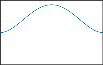
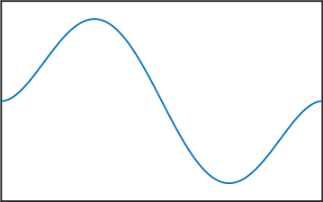
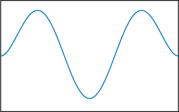
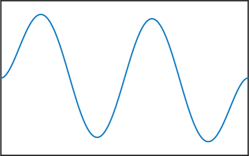
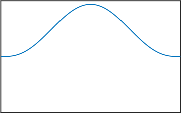
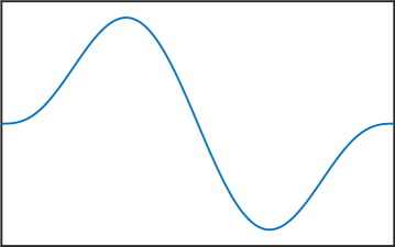
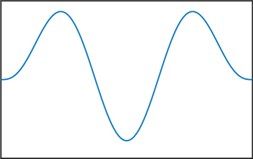
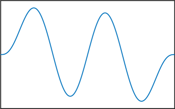
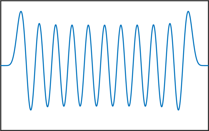
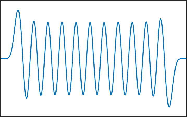
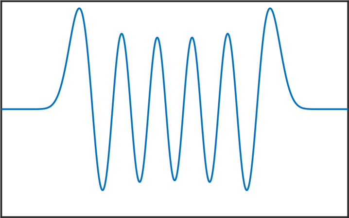
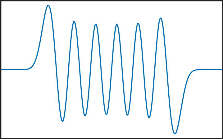
Melkman and Micchelli [17] proved that for all $r$ there exists an optimal space $X_{n}$ containing $C^{r-2}$ piecewise polynomials of degree $r-1$. The zeros of the eigenfunctions in (6) are exactly the internal knots of these spline spaces. Thus, the presented numerical method allows us to compute these knots, and as stated in the introduction, this can be very useful for Isogeometric Analysis [4]. See Figure 4 for various computed eigenfunctions in the case $m=500$.

Andrea Bressan was partially supported by the European Research Council through the FP7 Ideas Consolidator Grant HIGEOM n.616563, and by the Italian Ministry of Education, University and Research (MIUR) through the “Dipartimenti di Eccellenza Program (2018-2022) - Dept. of Mathematics, University of Pavia”. Espen Sande was supported by the Beyond Borders Programme of the University of Rome Tor Vergata through the project ASTRID (CUP E84I19002250005) and by the MIUR Excellence Department Project awarded to the Department of Mathematics, University of Rome Tor Vergata (CUP E83C18000100006). Andrea Bressan and Espen Sande are members of Gruppo Nazionale per il Calcolo Scientifico, Istituto Nazionale di Alta Matematica.

References

• [1] P. M. Anselone and J. W. Lee, Spectral properties of integral operators with nonnegative kernels, Linear Algebra and Appl. 9 (1974), 67–87.
• [2] K. Atkinson, Convergence rates for approximate eigenvalues of compact integral operators, SIAM J. Numer. Anal. 12 (1975), 213–222.
• [3] A. Bressan and E. Sande, Approximation in FEM, DG and IGA: a theoretical comparison, Numer. Math. 143 (2019), 923–942.
• [4] J. Chan and J. A. Evans, Multi-patch discontinuous Galerkin isogeometric analysis for wave propagation: explicit time-stepping and efficient mass matrix inversion, Comput. Methods Appl. Mech. Engrg. 333 (2018), 22–54.
• [5] F. Chatelin, The spectral approximation of linear operators with applications to the computation of eigenelements of differential and integral operators, SIAM review 23 (1981), 495–522.
• [6] G. Dahlquist and Å. Björck, Numerical methods in scientific computing: Volume 1, Society for Industrial and Applied Mathematics, 2008.
• [7] J. A. Evans, Y. Bazilevs, I. Babuska, and T. J. R. Hughes, n-Widths, sup-infs, and optimality ratios for the k-version of the isogeometric finite element method, Comput. Methods Appl. Mech. Engrg. 198 (2009), 1726–1741.
• [8] M. S. Floater and E. Sande, Optimal spline spaces of higher degree for L2L^{2} nn-widths, J. Approx. Theory 216 (2017), 1–15.
• [9]   , On periodic L2L^{2} nn-widths, J. Comput. Appl. Math. 349 (2019), 403–409.
• [10]   , Optimal spline spaces for L2L^{2} nn-width problems with boundary conditions, Constr. Approx. 50 (2019), 1–18.
• [11] A. Ioffe and V. M. Tihomirov, Duality of convex functions and extremum problems, Russian Math. Surveys 23 (1968), 53–124.
• [12] S. Karlin, Total positivity, Vol. I, Stanford University Press, Stanford, California, 1968.
• [13] L. A. Karlovitz, Remarks on variational characterizations of eigenvalues and n-width problems, J. Math. Anal. Appl. 53 (1976), 99–110.
• [14] A. Kolmogorov, Über die beste Annäherung von Funktionen einer gegebenen Funktionenklasse, Ann. of Math. 37 (1936), 107–110.
• [15] N. P. Korneichuk, Exact constants in approximation theory, Cambridge University press, Cambridge, 1991.
• [16] Tom Lyche and Knut Morken, Spline methods draft, 2011.
• [17] A. A. Melkman and C. A. Micchelli, Spline spaces are optimal for L2L^{2} nn-widths, Illinois J. Math. 22 (1978), 541–564.
• [18] C. A. Micchelli and A. Pinkus, On n-widths in L-infinity, Trans. Amer. Math. Soc. 234 (1977), 139–174.
• [19] J. E. Osborn, Spectral approximation for compact operators, Math. Comp. 29 (1975), 712–725.
• [20] A. Pinkus, n-Widths in approximation theory, Springer-Verlag, Berlin, 1985.
• [21] E. Sande, C. Manni, and H. Speleers, Sharp error estimates for spline approximation: Explicit constants, nn-widths, and eigenfunction convergence, Math. Models Methods Appl. Sci. 29 (2019), 1175–1205.
• [22] M. H. Schultz, Error bounds for polynomial spline interpolation, Math. Comp. 24 (1970), 507–515.
• [23] A. Yu. Shadrin, Inequalities of Kolmogorov type and estimates of spline interpolation on periodic classes W2mW^{m}_{2}, Mat. Zametki 48 (1990), 132–139.
• [24] V. M. Tikhomirov, Approximation theory, Analysis II: Convex Analysis and Approximation Theory (R. V. Gamkrelidze, ed.), Springer Berlin Heidelberg, 1990, pp. 93–243.