On evolution kernels of twist-two operators
Abstract
The evolution kernels that govern the scale dependence of the generalized parton distributions are invariant under transformations of the collinear subgroup of the conformal group. Beyond one loop the symmetry generators, due to quantum effects, differ from the canonical ones. We construct the transformation which brings the full symmetry generators back to their canonical form and show that the eigenvalues (anomalous dimensions) of the new, canonically invariant, evolution kernel coincide with the so-called parity respecting anomalous dimensions. We develop an efficient method that allows one to restore an invariant kernel from the corresponding anomalous dimensions. As an example, the explicit expressions for NNLO invariant kernels for the twist two flavor-nonsinglet operators in QCD and for the planar part of the universal anomalous dimension in SYM are presented.
I Introduction
The study of deeply-virtual Compton scattering (DVCS) gives one access to the generalized parton distributions [1, 2, 3] (GPDs) that encode the information on the transverse position of quarks and gluons in the proton in dependence on their longitudinal momentum. In order to extract the GPDs from experimental data one has to know, among other things, their scale dependence. The latter is governed by the renormalization group equations (RGEs) or, equivalently, evolution equations for the corresponding twist two operators. Essentially the same equations govern the scale dependence of the ordinary parton distribution functions (PDFs) in the Deep Inelastic Scattering (DIS) process. In DIS one is interested in the scale dependence of forward matrix elements of the local twist-2 operators and therefore can neglect the operator mixing problem between local operators from the operator product expansion (OPE). In the nonsinglet sector, there is only one operator for a given spin/dimension. The anomalous dimensions of such operators are known currently with the three-loop accuracy [4, 5] and first results at four loops are becoming available [6, 7]. In contrast, the DVCS process corresponds to non-zero momentum transfer from the initial to the final state and, as a consequence, the total derivatives of the local twist-two operators have to be taken into consideration. All these operators mix under renormalization and the RGE has a matrix form. The DIS anomalous dimensions appear as the diagonal entries of the anomalous dimensions matrix which, in general, has a triangular form for the latter.
It was shown by Dieter Müller [8, 9] that the off-diagonal part of the anomalous dimension matrix is completely determined by a special object, the so-called conformal anomaly. Moreover, in order to determine the off-diagonal part of the anomalous dimension matrix with -loop accuracy it is enough to calculate the conformal anomaly at one loop less. This technique was used to reconstruct all relevant evolution kernels/anomalous dimension matrices in QCD at two loops [10, 11, 12].
A similar approach, but based on the analysis of QCD at the critical point in non-integer dimensions, was developed in refs. [13, 14, 15]. It was shown that the evolution kernels in in the -like renormalization scheme inherit the symmetries of the critical theory in dimensions. As expected, the symmetry generators deviate from their canonical form. Corrections to the generators have a rather simple form if they are written in terms of the evolution kernel and the conformal anomaly. It was shown in ref. [16] that by changing a renormalization scheme one can get rid of the conformal anomaly term in the generators bringing them into the so-called “minimal” form. Beyond computing the evolution kernels, the conformal approach has also been employed to calculate the NNLO coefficient (hard) functions of vector and axial-vector contributions in DVCS [17, 18], the latter in agreement with a direct Feynman diagram calculation [19]. Moreover, the conformal technique is also applicable to computing kinematic higher-power corrections in two-photon processes as was recently shown in refs. [20, 21].
In this paper we construct a similarity transformation that brings the full quantum generators back to the canonical form. Correspondingly, the transformed evolution kernel is invariant under the canonical transformation. Moreover, we will show that the eigenvalues of this kernel are given by the so-called parity respecting anomalous dimension, [22, 23] which is related to the PDF anomalous dimension spectrum as
| (1) |
where with being the QCD beta function. The strong coupling is normalized as . We develop an effective approach to restore the canonically invariant kernel from its eigenvalues . As an example, we present explicit expressions for three-loop invariant kernels in QCD and supersymmetric Yang-Mills (SYM) theory. The answers are given by linear combinations of harmonic polylogarithms [24], up to weight four in QCD and up to weight three in SYM. We also compare our exact result with the approximate expression for the three-loop kernels in QCD given in ref. [16].
The paper is organized as follows: in section II we describe the general structure of the evolution kernels of twist-two operators. In section III we explain how to effectively recover the evolution kernel from the known anomalous dimensions and present our results for the invariant kernels in QCD and SYM. Sect. IV contains the concluding remarks. Some technical details are given in the Appendices.
II Kernels & symmetries
We are interested in the scale dependence of the twist-two light-ray flavor nonsinglet operator [25]
| (2) |
where is an auxiliary light-like vector, , are real numbers, and stands for the Wilson line ensuring gauge invariance, and the subscript denotes the renormalization scheme. This operator can be viewed as the generating function for local operators, that are symmetric and traceless in all Lorentz indices .
The renormalized light-ray operator (2) satisfies the RGE
| (3) |
where is -dimensional beta function
| (4) |
, etc., and is an integral operators in .
It follows from the invariance of the classical QCD Lagrangian under conformal transformations that the one-loop kernel commutes with the canonical generators of the collinear conformal subgroup, ,
| (5) |
This symmetry is preserved beyond one loop albeit two of the generators, receive quantum corrections, . The explicit form of these corrections can be found in ref. [15].
It is quite useful to bring the generators to the following form using the similarity transformation [16],
| (6) |
where is an integral operator known up to terms of [11, 16]. This transformation can be thought of as a change in a renormalization scheme.
The shift operator is not modified and hence identical to in Eq. (II), and the quantum corrections to and come only through the evolution kernel
| (7a) | ||||
| (7b) | ||||
where is the beta function in four dimensions, cf. Eq. (1). The form of the generator is completely fixed by the scale invariance of the theory, while Eq. (7b) is the “minimal” ansatz consistent with the commutation relation . Since the operator commutes with the generators, its form is completely determined by its spectrum (anomalous dimensions). However, since the generators do not have the simple form as in Eq. (II), it is yet necessary to find a way to recover the operator from its spectrum.
To this end we construct a transformation which brings the generators to the canonical form , Eq. (II). Let us define an operator :
| (8) |
where , . Recall that are real variables, so for it is necessary to choose a specific branch of the logarithm function. Although this choice is irrelevant for further analysis we chose the recipe for concreteness, i.e., . It can be shown that the operator intertwines the symmetry generators and the canonical generators, . Namely,
| (9) |
see Appendix A for details. Let us also define a new kernel as
| (10) |
It follows from Eqs. (9), (10) that the operator commutes with the canonical generators in Eq. (II)
| (11) |
The problem of restoring a canonically invariant operator from its spectrum is much easier than that for the operator and will be discussed in the next section. It can be shown that the inverse of takes the form
| (12) |
see Appendix A. Further, it follows from Eq. (10) that
| (13) |
The operators are defined by recursion
| (14) |
with the boundary condition . The -th term in the sum in Eq. (II) is of order so that one can easily work out an approximation for with arbitrary precision, e.g.,
| (15) |
It can be checked that this expression coincides with that obtained in ref. [16, Eq. (3.9)] ***The notations adopted here and in ref. [16] differ slightly. To facilitate a comparison we note that the operators defined here satisfy the equation ..
The evolution kernel can be realized as an integral operator. It acts on a function of two real variables as follows
| (16) |
where is a constant, , , and
| (17) |
is called conformal ratio. The weight function in Eq. (16) only depends on this particular combination of the variables as a consequence of invariance properties of , Eq. (11).
III Anomalous dimensions vs kernels
First of all let us establish a connection between the eigenvalues of the operators and . Since both of them are integral operators of the functional form in Eqs. (16), (18), both operators are diagonalized by functions of the form , where is an arbitrary complex number. One may worry that the continuation of the function for negative is not unique and requires special care. But it does not matter for our analysis. Indeed, with , therefore the operators do not mix the regions . For definiteness let us suppose that
| (19) |
Let be eigenvalues (anomalous dimensions) of the operators , corresponding to the function , respectively,
| (20) | ||||
| (21) |
The anomalous dimensions are analytic functions of in the right complex half-plane, . For integer even (odd) , gives the anomalous dimensions of the local (axial)vector operators †††As usual one has to consider the operators of certain parity, , then the functions give the anomalous dimensions of local operators, for even and odd respectively..
Now let us note that the operator acts on as follows
| (22) |
Thus, it follows from Eq. (II) that the anomalous dimensions and satisfy the relation (cf. also Eq. (1))
| (23) |
This relation appeared first in refs. [23, 22] as an generalization of the Gribov-Lipatov reciprocity relation [26, 27]. It was shown that the asymptotic expansion of the function for large is invariant under the reflection , see e.g., refs. [22, 28, 29, 30]. This property strongly restricts harmonics sums which can appear in the perturbative expansion of the anomalous dimension [29]. Explicit expressions for are known at four loops in QCD [6] and at seven loops in the SYM, see refs. [31, 29, 32, 33, 34].
III.1 Kernels from anomalous dimensions
For large the anomalous dimension grows as . This term enters with a coefficient where is the so-called cusp anomalous dimension [35, 36] whose complete form is known to the four-loop order in QCD [37, 38] and in SYM [37]. In the planar limit of SYM, the cusp anomalous dimension is known beyond the four-loop order (e.g., as a special case of results in [33, 34]), and in fact, to any loop order from ref. [39]. Thus, we write in the following form
| (24) |
where is the harmonic sum responsible for the behavior at large , and is a constant term. The remaining term, , vanishes at least as at large . The constant is exactly the same which appears in Eq. (16). The first term in Eq. (24) comes from a special invariant kernel
| (25) |
which in momentum space gives rise to the so-called plus-distribution. The eigenvalues of this kernel are (). It corresponds to a singular contribution of the form to the invariant kernel , see ref. [16, Eq. (2.19)] for detail. Thus the evolution kernel can be generally written as
| (26) |
Here is an integral operator,
| (27) |
where the weight function is a regular function of . The eigenvalues of are equal to and are given by the following integral
| (28) |
The inverse transformation takes the form [14]
| (29) |
where are the Legendre polynomials. The integration path goes along the line parallel to the imaginary axis, , such that all poles of lie to the left of this line. Some details of the derivation can be found in Appendix B.
One can hardly hope to evaluate the integral (29) in a closed form for an arbitrary function . However, as was mentioned before, the anomalous dimensions in quantum field theory are rather special functions. Most of the terms in the perturbative expansion of have the following form
| (30) |
where , and the functions are the parity respecting harmonic sums [29], ( for ). We will assume that the sums are “subtracted”, i.e. at . The second structure occurs only for , since grows as for large .
Since all invariant operators share the same eigenfunctions, the product of two invariant operators and , with eigenvalues and respectively, has eigenvalues . One can use this property to reconstruct an operator with the eigenvalue (30).
First, we remark that the operator with the eigenvalues , (we denote it as ), has (as follows from Eq. (28)) a very simple weight function, . This can also be derived from Eq. (29). Since the integral in Eq. (29) vanishes for the integration path due to antisymmetry of the integrand. Therefore, the integral (29) can be evaluated by the residue theorem ‡‡‡This trick allows one to calculate the integral (29) for any function with exact symmetry under reflection.
| (31) |
Let us consider the product , where is an integral operator with the weight function . Then the weight function of the operator is given by the following integral
| (32) |
see Appendix B for details. Thus the contribution to the anomalous dimension of type (30) can be evaluated with the help of this formula if the weight function corresponding to the harmonic sums is known.
We also give an expression for another product of the operators: ,
| (33) |
which appears to be useful in the calculations as well.
III.2 Recurrence procedure
Let us consider the integral (29) with ,
| (34) |
where . Using a recurrence relation for the Legendre functions
| (35) |
we obtain
| (36) |
where
| (37) |
It is easy to see that the function has the negative parity under transformation and can be represented in the form
| (38) |
where are rational functions of . The harmonic sums in Eq. (38) can be either of positive or negative parity. Therefore the coefficient accompanying the positive parity function has the form , where is some polynomial, while for the harmonic sums of negative parity. The free term has the form . Together, they make with negative parity. For example, for the harmonic sum (see appendix C for a definition), one gets
| (39) |
while for the harmonic sum
| (40) |
Note the reappearance of the common factor in the first case, (39). This implies that, up to the derivative , the integral (36) has the form (29). Hence, if the kernel corresponding to the underlined terms in Eq. (39) is known, the kernel corresponding to can be easily obtained. Thus the problem of finding the invariant kernel with the eigenvalues is reduced to the problem of finding the kernel with the eigenvalues .
However, as it seen from our second example, not all parity preserving harmonic sums share this property. Indeed, the underlined term on the right hand side (rhs) of Eq. (40) does not have the factor . Hence, all these transformations do not help to solve the problem for .
It is easy to see that the above recurrence procedure works only if all the harmonic sums appearing in Eq. (38) are of positive parity. It was proven in ref. [29, Theorem 2] that any harmonic sum, , with all indices positive odd or negative even has positive parity (see Appendix C for explicit examples of the harmonic sums satisfying these conditions). Therefore, the rhs of Eq. (38) only contains harmonic sums of the same type. Thus the invariant kernels corresponding to the harmonic sums of positive parity can always be calculated recursively, using Eqs. (36), (38) and (32), (33). Crucially, only such harmonic sums appear in the anomalous dimensions in QCD and SYM. All convolution integrals (32) and (33) can in turn be systematically calculated with the packages HyperInt [40] or PolyLogTools [41].
The explicit expressions for the kernels corresponding to the lowest harmonic sums are given in Appendix C for references.
III.3 Invariant kernels: QCD
Below we give an explicit expression for the invariant kernel of twist-two flavor nonsinglet operator in QCD. We will not split the operator into positive (negative) parity operators. The evolution operator still takes the form (26), with given by the following integral
| (41) |
where is a permutation operator, §§§ In order to avoid possible misunderstandings we write down it explicitly, .. For (anti)symmetric functions the operator (41) takes a simpler form (27) with the kernel .
Our expression for the constant term agrees with the constant term given in ref. [16, Eq. (5.5)], . For completeness, we provide explicit expressions for the constant ,
| (42) |
where is the quadratic Casimir in the fundamental representation of and we take . Note that we are adopting a different color basis compared to ref. [16].
The explicit expressions for the cusp anomalous dimensions up to three loops are provided in Eq. (D). Finally we give answers for the kernels . Explicit one- and two-loop expressions are known [14, 16] but for completeness we give them here
| (43) |
and
| (44) |
where are the harmonic polylogarithms (HPLs) [24]. The three-loop expression¶¶¶A file with our main results can be obtained from the preprint server http://arXiv.org by downloading the source. Furthermore, they are available from the authors upon request. is more involved
| (45) | ||||
| and | ||||
| (46) | ||||
The kernels are smooth functions of except for the endpoints and . For the three-loop kernel functions behave as . For small – which determines the large asymptotic of the anomalous dimensions – the kernels (for each color structure) have the form . We note here that the reciprocity property of the anomalous dimension is equivalent to the statement that the small expansion of the kernels does not involve non-integer powers of , namely .
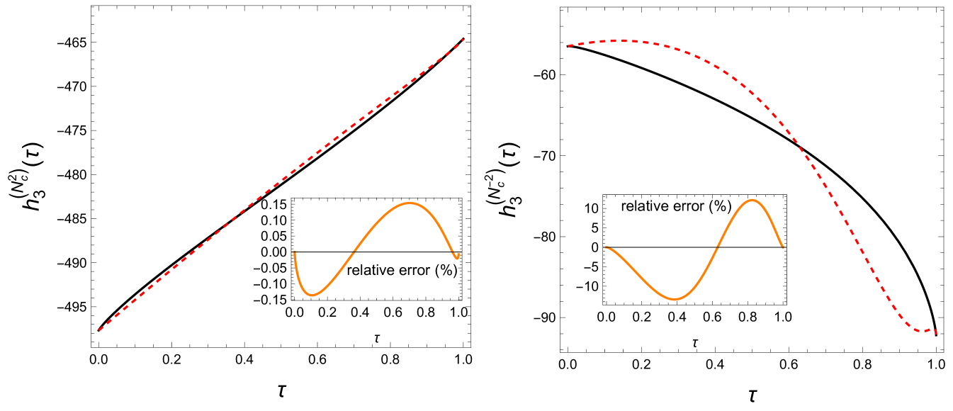
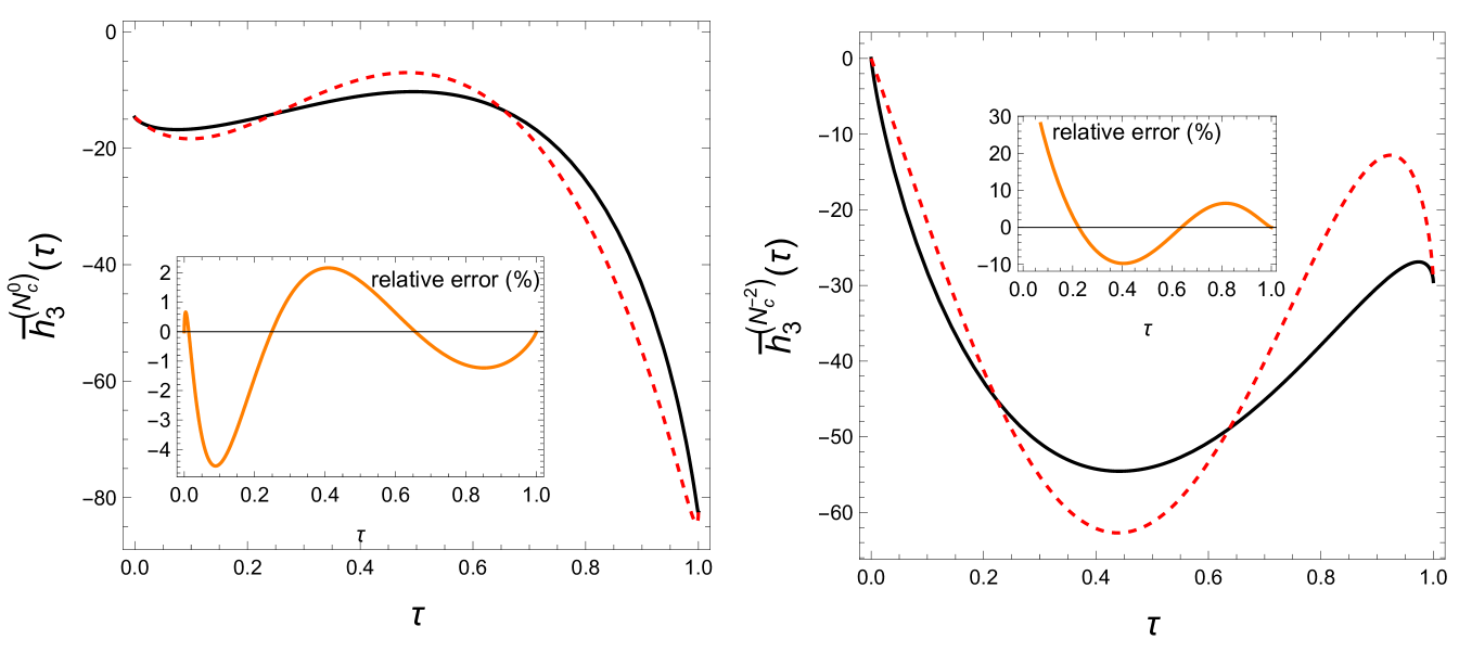
Below we compare our exact three-loop results with the approximate expressions constructed in ref. [16]. The approximate expressions reproduce the asymptotic behaviors of the exact kernels at both . We therefore subtract the logarithmically divergent pieces (see Eqs. (D) and (D) for explicit expressions) from both the exact and the approximated expressions to highlight their (small) deviations as shown in Figs. 1 and 2. For illustrative purposes, we plot the planar contribution ( and in and respectively) and the subsubplanar contribution (). The former is numerically dominant and generates the leading contribution in the large- limit whereas the latter shows the worst-case scenario for the previous approximation using a simple HPL function ansatz. The error of other color structures all fall between the planar and subsubplanar cases, hence are numerically small.
III.4 Invariant kernels: SYM
In this section we present the invariant kernels for the universal anomalous dimensions of the planar SYM, see e.g., refs. [42, 31] for expressions up to NNLO. They are rather short so that we quote them here. We use the parametrization (24), where can be found in ref. [37] and the constant term is
| (47) |
where , and
| (48) |
For the kernels we find ,
| (49) |
and
| (50) | ||||
These expressions are extremely simple in comparison with the expressions in QCD of the same order. Let us notice that the two-loop kernels contain only HPLs of weight one with the three-loop kernels involving HPLs of weight three, while in QCD the corresponding kernels require HPLs of weight two and four, respectively. Note also that the kernel is proportional to the factor and the kernel to the factor . It would be interesting to see if these properties persist in higher loops.
IV Summary
We have constructed a transformation that brings the evolution kernels of twist-two operators to the canonically conformal invariant form. The eigenvalues of these kernels are given by the parity respecting anomalous dimensions. We have developed a recurrence procedure that allows one to restore the weight functions of the corresponding kernels. It is applicable to a subset of the harmonic sums (with positive odd and negative even indices). It is interesting to note that exactly only such harmonic sums appear in the expressions for the reciprocity respecting anomalous dimensions.
We have calculated the three-loop invariant kernels in QCD and in SYM (in the planar limit). In QCD it was the last missing piece to obtain the three-loop evolution kernels for the flavor-nonsinglet twist-two operators in a fully analytic form, see ref. [16].
In the case of SYM the lowest order expressions for the kernels are rather simple and exhibit some regularities, , . It would be interesting to check if these properties survive at higher loops. We expect that at -loops the kernels will be given by linear combinations (up to common prefactors) of HPLs of weight with positive indices. Therefore going over to the invariant kernel can lead to a more compact representation of the anomalous dimensions than representing the anomalous dimension spectrum in terms of harmonic sums. The much smaller function basis in terms of HPLs ( and ) opens the possibility of extracting the analytical expressions of the higher-order evolution kernels from minimal numerical input through the PSLQ algorithm.
Acknowledgments
We are grateful to Vladimir M. Braun and Gregory P. Korchemsky for illuminating discussions and comments on the manuscript. This work is supported by Deutsche Forschungsgemeinschaft (DFG) through the Collaborative Research Center TRR110/2, grant 409651613 (Y.J.), and the Research Unit FOR 2926, project number 40824754 (S.M.).
Appendices
Appendix A
In this appendix, we describe in detail the derivations of some of the equations presented in section II. Let us start with Eq. (9). For the generator the statement is trivial. Next, making use of Eq. (8) for the operator and, taking into account that commutes with the generators , one can write the left hand side (lhs) of Eq. (9) in the form
| (A.51) |
where . Using the representation (7) for the generators and taking into account that and (we recall that ) one obtains
| (A.52) |
Substituting these expressions back into Eq. (A.51) one finds that the contributions of the last two terms on the rhs of Eq. (A) cancel each other. Hence Eq. (A.51) takes the form
| (A.53) |
that finally results in Eq. (9).
Let us now show that the inverse to has the form (12). The product can be written as
| (A.54) |
Moving to the left with help of the relation (10) and then using Eq. (8) for one gets ()
Finally, we consider the product of operators with a differently defined function . Namely, let us take , where so that . In order to calculate the product one proceeds as before: use expansion (8) for , move to the left and then expand it into a power series. It yields
| (A.55) |
where . Let one can get for the sum in Eq. (A.55)
where . Since one concludes that commutes with the canonical generators and hence .
Appendix B
Let us check that the kernel given by Eq. (29) has the eigenvalues . First, after some algebra, the integral in Eq. (28) can be brought to the following form
| (B.56) |
where is the Legendre function of the second kind [43]. Inserting in the form of Eq. (29) into Eq. (B.56) one gets
| (B.57) |
The -integral of the product of the two Legendre functions gives [43]
| (B.58) |
Then closing the integration contour in the right half-plane one evaluates the integral with the residue theorem at yielding the desired lhs of Eq. (B.56).
Appendix C
In this appendix, we collect the harmonic sums and the corresponding kernels which we have used. We split them into two parts: the first one includes the harmonic sums such that .
| (C.60) |
Here are the harmonic sums with argument . We define the sums of negative signature, , with an additional sign factor:
| (C.61) |
These combinations of harmonic sums are generated by the following kernels,
| (C.62) |
and
| (C.63) |
where all HPLs have argument . These functions serve as a basis and more complicated structures can be generated as products of .
Appendix D
Here we give the small () and large ( expansions of the invariant kernels . By () we denote the function which appears in the expression for () with the color factor . We will keep the logarithmically enhanced and constant terms in both limits. The former is subtracted from both the exact and approximated three-loop kernel to obtain the two figures in Eqs. 1 and 2. At one gets
| (D.64) |
and for one obtains
| (D.65) |
References
- Müller et al. [1994] D. Müller, D. Robaschik, B. Geyer, F. M. Dittes, and J. Hořejši, Wave functions, evolution equations and evolution kernels from light ray operators of QCD, Fortsch. Phys. 42, 101 (1994), arXiv:hep-ph/9812448 .
- Radyushkin [1996] A. V. Radyushkin, Scaling limit of deeply virtual Compton scattering, Phys. Lett. B380, 417 (1996), arXiv:hep-ph/9604317 [hep-ph] .
- Ji [1997] X.-D. Ji, Deeply virtual Compton scattering, Phys. Rev. D55, 7114 (1997), arXiv:hep-ph/9609381 [hep-ph] .
- Moch et al. [2004] S. Moch, J. A. M. Vermaseren, and A. Vogt, The Three loop splitting functions in QCD: The Nonsinglet case, Nucl. Phys. B 688, 101 (2004), arXiv:hep-ph/0403192 .
- Vogt et al. [2004] A. Vogt, S. Moch, and J. A. M. Vermaseren, The Three-loop splitting functions in QCD: The Singlet case, Nucl. Phys. B 691, 129 (2004), arXiv:hep-ph/0404111 .
- Moch et al. [2017] S. Moch, B. Ruijl, T. Ueda, J. A. M. Vermaseren, and A. Vogt, Four-Loop Non-Singlet Splitting Functions in the Planar Limit and Beyond, JHEP 10, 041, arXiv:1707.08315 [hep-ph] .
- Falcioni et al. [2023] G. Falcioni, F. Herzog, S. Moch, and A. Vogt, Four-loop splitting functions in QCD – The quark-quark case –, Phys. Lett. B 842, 137944 (2023), arXiv:2302.07593 [hep-ph] .
- Müller [1991] D. Müller, Constraints for anomalous dimensions of local light cone operators in in six-dimensions theory, Z. Phys. C 49, 293 (1991).
- Müller [1998] D. Müller, Restricted conformal invariance in QCD and its predictive power for virtual two photon processes, Phys. Rev. D 58, 054005 (1998), arXiv:hep-ph/9704406 .
- Belitsky and Müller [1998] A. V. Belitsky and D. Müller, Predictions from conformal algebra for the deeply virtual Compton scattering, Phys. Lett. B417, 129 (1998), arXiv:hep-ph/9709379 [hep-ph] .
- Belitsky and Müller [1999] A. V. Belitsky and D. Müller, Broken conformal invariance and spectrum of anomalous dimensions in QCD, Nucl. Phys. B 537, 397 (1999), arXiv:hep-ph/9804379 .
- Belitsky et al. [2000] A. V. Belitsky, A. Freund, and D. Müller, Evolution kernels of skewed parton distributions: Method and two loop results, Nucl. Phys. B 574, 347 (2000), arXiv:hep-ph/9912379 .
- Braun and Manashov [2013] V. M. Braun and A. N. Manashov, Evolution equations beyond one loop from conformal symmetry, Eur. Phys. J. C 73, 2544 (2013), arXiv:1306.5644 [hep-th] .
- Braun and Manashov [2014] V. M. Braun and A. N. Manashov, Two-loop evolution equations for light-ray operators, Phys. Lett. B 734, 137 (2014), arXiv:1404.0863 [hep-ph] .
- Braun et al. [2016] V. M. Braun, A. N. Manashov, S. Moch, and M. Strohmaier, Two-loop conformal generators for leading-twist operators in QCD, JHEP 03, 142, arXiv:1601.05937 [hep-ph] .
- Braun et al. [2017] V. M. Braun, A. N. Manashov, S. Moch, and M. Strohmaier, Three-loop evolution equation for flavor-nonsinglet operators in off-forward kinematics, JHEP 06, 037, arXiv:1703.09532 [hep-ph] .
- Braun et al. [2020] V. M. Braun, A. N. Manashov, S. Moch, and J. Schönleber, Two-loop coefficient function for DVCS: vector contributions, JHEP 09, 117, arXiv:2007.06348 [hep-ph] .
- Braun et al. [2021a] V. M. Braun, A. N. Manashov, S. Moch, and J. Schönleber, Axial-vector contributions in two-photon reactions: Pion transition form factor and deeply-virtual Compton scattering at NNLO in QCD, Phys. Rev. D 104, 094007 (2021a), arXiv:2106.01437 [hep-ph] .
- Gao et al. [2022] J. Gao, T. Huber, Y. Ji, and Y.-M. Wang, Next-to-Next-to-Leading-Order QCD Prediction for the Photon-Pion Form Factor, Phys. Rev. Lett. 128, 062003 (2022), arXiv:2106.01390 [hep-ph] .
- Braun et al. [2021b] V. M. Braun, Y. Ji, and A. N. Manashov, Two-photon processes in conformal QCD: resummation of the descendants of leading-twist operators, JHEP 03, 051, arXiv:2011.04533 [hep-ph] .
- Braun et al. [2023] V. M. Braun, Y. Ji, and A. N. Manashov, Next-to-leading-power kinematic corrections to DVCS: a scalar target, JHEP 01, 078, arXiv:2211.04902 [hep-ph] .
- Basso and Korchemsky [2007] B. Basso and G. P. Korchemsky, Anomalous dimensions of high-spin operators beyond the leading order, Nucl. Phys. B 775, 1 (2007), arXiv:hep-th/0612247 .
- Dokshitzer et al. [2006] Y. L. Dokshitzer, G. Marchesini, and G. P. Salam, Revisiting parton evolution and the large-x limit, Phys. Lett. B 634, 504 (2006), arXiv:hep-ph/0511302 .
- Remiddi and Vermaseren [2000] E. Remiddi and J. A. M. Vermaseren, Harmonic polylogarithms, Int. J. Mod. Phys. A 15, 725 (2000), arXiv:hep-ph/9905237 .
- Balitsky and Braun [1989] I. I. Balitsky and V. M. Braun, Evolution Equations for QCD String Operators, Nucl. Phys. B 311, 541 (1989).
- Gribov and Lipatov [1972a] V. N. Gribov and L. N. Lipatov, Deep inelastic e p scattering in perturbation theory, Sov. J. Nucl. Phys. 15, 438 (1972a).
- Gribov and Lipatov [1972b] V. N. Gribov and L. N. Lipatov, pair annihilation and deep inelastic scattering in perturbation theory, Sov. J. Nucl. Phys. 15, 675 (1972b).
- Dokshitzer and Marchesini [2007] Y. L. Dokshitzer and G. Marchesini, SUSY Yang-Mills: three loops made simple(r), Phys. Lett. B 646, 189 (2007), arXiv:hep-th/0612248 .
- Beccaria and Forini [2009] M. Beccaria and V. Forini, Four loop reciprocity of twist two operators in SYM, JHEP 03, 111, arXiv:0901.1256 [hep-th] .
- Alday et al. [2015] L. F. Alday, A. Bissi, and T. Lukowski, Large spin systematics in CFT, JHEP 11, 101, arXiv:1502.07707 [hep-th] .
- Kotikov et al. [2009] A. V. Kotikov, A. Rej, and S. Zieme, Analytic three-loop Solutions for SYM Twist Operators, Nucl. Phys. B 813, 460 (2009), arXiv:0810.0691 [hep-th] .
- Beccaria et al. [2009] M. Beccaria, V. Forini, T. Lukowski, and S. Zieme, Twist-three at five loops, Bethe Ansatz and wrapping, JHEP 03, 129, arXiv:0901.4864 [hep-th] .
- Marboe et al. [2015] C. Marboe, V. Velizhanin, and D. Volin, Six-loop anomalous dimension of twist-two operators in planar SYM theory, JHEP 07, 084, arXiv:1412.4762 [hep-th] .
- Marboe and Velizhanin [2016] C. Marboe and V. Velizhanin, Twist-2 at seven loops in planar SYM theory: full result and analytic properties, JHEP 11, 013, arXiv:1607.06047 [hep-th] .
- Polyakov [1980] A. M. Polyakov, Gauge Fields as Rings of Glue, Nucl. Phys. B 164, 171 (1980).
- Korchemsky and Radyushkin [1987] G. P. Korchemsky and A. V. Radyushkin, Renormalization of the Wilson Loops Beyond the Leading Order, Nucl. Phys. B 283, 342 (1987).
- Henn et al. [2020] J. M. Henn, G. P. Korchemsky, and B. Mistlberger, The full four-loop cusp anomalous dimension in super Yang-Mills and QCD, JHEP 04, 018, arXiv:1911.10174 [hep-th] .
- von Manteuffel et al. [2020] A. von Manteuffel, E. Panzer, and R. M. Schabinger, Cusp and collinear anomalous dimensions in four-loop QCD from form factors, Phys. Rev. Lett. 124, 162001 (2020), arXiv:2002.04617 [hep-ph] .
- Beisert et al. [2007] N. Beisert, B. Eden, and M. Staudacher, Transcendentality and Crossing, J. Stat. Mech. 0701, P01021 (2007), arXiv:hep-th/0610251 .
- Panzer [2015] E. Panzer, Algorithms for the symbolic integration of hyperlogarithms with applications to Feynman integrals, Comput. Phys. Commun. 188, 148 (2015), arXiv:1403.3385 [hep-th] .
- Duhr and Dulat [2019] C. Duhr and F. Dulat, PolyLogTools — polylogs for the masses, JHEP 08, 135, arXiv:1904.07279 [hep-th] .
- Kotikov et al. [2003] A. V. Kotikov, L. N. Lipatov, and V. N. Velizhanin, Anomalous dimensions of Wilson operators in SYM theory, Phys. Lett. B 557, 114 (2003), arXiv:hep-ph/0301021 .
- Gradshteyn and Ryzhik [1994] I. S. Gradshteyn and I. M. Ryzhik, Table of integrals, series, and products, russian ed. (Academic Press, Inc., Boston, MA, 1994) pp. xlviii+1204, translation edited and with a preface by Alan Jeffrey.