On finite type invariants of welded string links and ribbon tubes
Abstract.
Welded knotted objects are a combinatorial extension of knot theory, which can be used as a tool for studying ribbon surfaces in -space. A finite type invariant theory for ribbon knotted surfaces was developed by Kanenobu, Habiro and Shima, and this paper proposes a study of these invariants, using welded objects. Specifically, we study welded string links up to -equivalence, which is an equivalence relation introduced by Yasuhara and the second author in connection with finite type theory. In low degrees, we show that this relation characterizes the information contained by finite type invariants. We also study the algebraic structure of welded string links up to -equivalence. All results have direct corollaries for ribbon knotted surfaces.
Key words and phrases:
welded knotted objects, ribbon knotted surfaces in -space, finite type invariants1991 Mathematics Subject Classification:
57M27, 57M25, 57Q451. Introduction
In the study of knotted surfaces, i.e. smooth embeddings of -dimensional manifolds in -space, the class of ribbon surfaces has proved to be of particular interest. These are the analogue of ribbon knots in -space, as defined by Fox in the sixties, in the sense that such knotted surfaces bound immersed -manifolds with only one fixed topological type of so-called ribbon singularities. Ribbon knotted surfaces were extensively studied from the early days higher dimensional knot theory, notably through the work of Yajima [18, 19] and Yanagawa [21, 22, 20]. One nice feature of ribbon knotted surfaces is that they admit a natural notion of ’crossing change’. Indeed, one can always arrange such surfaces so that the only crossings occur along circles of double points: swapping the over/under information along such a circle then yields a new ribbon surface. Just like the usual crossing change can be used to define Vassiliev knot invariants, Kanenobu, Habiro and Shima used this local move to introduce a theory of finite type invariants for ribbon knotted surfaces [7, 8]. For ribbon -knots, Habiro and Shima further showed that finite type invariants are completely determined by the (normalized) Alexander polynomial.
This paper aims at characterizing, in a similar way, finite type invariants of ribbon tubes, which are ribbon knotted annuli in the -ball whose boundary is given by fixed copies of the unlink. These objects were introduced in [1], as a higher dimensional analogue of string links. For -component ribbon tubes, the situation is strictly the same as for ribbon -knots, in the sense that all finite type invariants come from the coefficients ) of the normalized Alexander polynomial [13]. For ribbon tubes of more components, a number of finite type invariants can be derived from this polynomial, as follows. Given a sequence of possibly overlined indices, there is a canonical procedure to connect the various components of a ribbon tube into a single annulus, and evaluating on the latter yields a degree finite type invariant of the initial ribbon tube, called a closure invariant, see Definition 2.16. Another family of finite type invariants of ribbon tubes is given by the higher-dimensional Milnor invariants defined in [1]. The first of these invariants is Milnor invariant , which in effect is the (nonsymmetric) linking number of component with component . The main result of this paper can be stated as follows.
Theorem 1.1.
Let and be two -component ribbon tubes. The following are equivalent for .
-
(1)
and are -equivalent.
-
(2)
For any finite type invariant of degree , we have .
-
(3)
and cannot be distinguished by the following invariants:
-
If : linking numbers , for all .
-
If : linking numbers for all , and closure invariants for all , , and for all , and for all pairwise distinct such that .
-
Here, the -equivalence is an equivalence relation introduced by Watanabe in [17] which, by the above, characterizes the information contained by finite type invariants of ribbon tubes of degree . This relation, discussed in Section 5, is an analogue in higher dimensions of Habiro’s -equivalence for usual knotted objects [6]. Watanabe showed that for ribbon –knots, the -equivalence characterizes the information contained by all finite type invariants of degree [17, Thm. 1.1].
Note that according to Theorem 1.1, any degree invariant of ribbon tubes can be expressed as a combination of linking numbers and closure invariants: we give such a formula for length Milnor invariants in Proposition 4.6. Note also that the case above was essentially already known by [2], see [13, § 7.2].
In Section 4.2, we investigate degree invariants in the -component case. The classification result is only given modulo a conjectured relation, but it appears already at this stage that closure invariants no longer suffice to generate all degree invariants, since the classification also involves length Milnor invariants. See Remark 4.15. An extensive study of degree invariants of ribbon tubes, and discussions on the perspectives that it opens, can be found in [3].
The results of this paper on ribbon knotted surfaces are all obtained as consequences of diagrammatic results. Another remarkable feature of ribbon surfaces is indeed that they can be described and studied using welded objects, which are a quotient of virtual knot theory, see Section 2.1. Early works of Yajima [18] highlighted the fact that all relations in the fundamental group of the complement of a ribbon –knot can be encoded using the usual diagrammatics of knot theory. This key observation was later completed and formalized by Satoh, as a surjective map from welded objects to ribbon knotted surfaces [16]. Hence the core of the present paper is a characterization of finite type invariants of welded string links. The theory of finite type invariants for welded objects is based on the virtualization move, which replaces a classical crossing by a virtual one, and the above-mentioned closure and Milnor invariants do have a strict analogue for welded string links, with the same finite type properties, see Section 2.3..
Our main tool will be the arrow calculus developed in [13], which is a welded analogue of Habiro’s clasper calculus [6]. In particular, a family of finer and finer equivalence relations on welded objects called -equivalence is defined in [13], which is closely related to finite type theory. It is indeed known that two -equivalent welded objects cannot be distinguished by any finite type invariant of degree . The converse implication also holds for welded (long) knots, thus fully characterizing the information contained by finite type invariants of these objects, and it is conjectured that such an equivalence also holds for welded string links (Conjecture 3.3). This is a natural analogue of the Goussarov-Habiro conjecture for finite type invariants of string links and homology cylinders [6] and, as a matter of fact, our results amount to verify this conjecture at low degree. Indeed, our main diagrammatical results are classifications of welded string links up to -equivalence for by finite type invariants (Corollary 4.4), which imply Theorem 1.1 as seen in Section 5. Several general results are also given on the set of -equivalence classes of welded string links, showing in particular that these form a finitely generated, non abelian group.
We conclude this introduction by mentioning the recent work of Colombari, who gave a complete classification of welded string links up to -concordance, for all , in [4]. This equivalence relation, generated by -equivalence and welded concordance, turns out to completely characterize welded string links (hence, classical string links) having the same Milnor invariants of length . This result also shows that all finite type concordance invariants of welded string links are given by Milnor invariants.
The rest of this paper is organized as follows. In Section 2.1, we review the notion of welded knotted objects and the basics of arrow calculus. Section 3 is devoted to the -equivalence; some algebraic properties of welded string links up to -equivalence are given in Section 3.3. Finite type invariants of welded string links are characterized at low degree in Section 4. The topological counterparts of our results, including the proof of Theorem 1.1, are given in the final Section 5.
2. Welded objects and arrow calculus
2.1. Welded knotted objects
Recall that a virtual diagram is a planar immersion of some -dimensional manifold; the singular set is a finite collection of transverse double points endowed with a decoration, either as a classical or as a virtual crossing. In figures, classical crossings are represented as in usual knot diagrams, while virtual crossings are simply drawn as double points (we do not follow the customary convention using circled double points).
Definition 2.1.
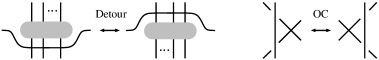
A welded knotted object is the equivalence class of a virtual diagram modulo the generalized Reidemeister moves and the OC move. Here the generalized Reidemeister moves consist of the three usual Reidemeister moves (involving classical crossings), and the Detour move shown in Figure 2.1. The OC move is shown on the right-hand side of the same figure.
Recall that usual (string) links inject into welded (string) links, in the sense that two diagrams without virtual crossings, that are related by a sequence of generalized Reidemeister and OC moves, represent isotopic objects, see [5, Thm 1.B]. Welded objects are also intimately related to ribbon knotted surfaces in -space, via Satoh’s Tube map [16], as further developed in Section 5.
Remark 2.2.
This paper will mainly deal with the following class
Definition 2.3.
An -component welded string link is the welded class of properly immersed copies of the unit interval into , endowed with fixed points on (), such that the th copy of the interval runs from the th fixed point in to the th fixed point in . A -component welded string link is also called a welded long knot.
We denote by the set of welded string links. The stacking product endows with a monoid structure, whose unit is given by the trivial diagram of intervals, with no crossing.
2.2. Arrow calculus
We now review the diagrammatic calculus for welded objects developed in [13], called arrow calculus. This is a welded analogue of Habiro’s clasper calculus for usual knotted objects [6] and, as such, it is intimately related to finite type invariants, see Section 2.3.3. Let be some welded knotted object.
Definition 2.4.
A -tree for is a connected unitrivalent tree , immersed into the plane so that
-
trivalent vertices are endowed with a cyclic order, are pairwise disjoint and disjoint from ;
-
univalent vertices are pairwise disjoint and lie in ;
-
edges are oriented, so that each trivalent vertex involves exactly one outgoing edge;
-
edges may contain virtual (but not classical) crossings, either with or with itself;
-
edges may contain decorations , called twists, which are subject to the involutive rule that two consecutive twists do cancel.
Moreover, for a union of Ðtrees for , we assume that vertices are pairwise disjoint, and that crossings among edges are all virtual.
We shall call tails and head the endpoints of a -tree, according to the orientation.
Definition 2.5.
The degree of a -tree is the number of tails. For , we call -tree a -tree of degree .
Now, a -tree is an instruction for modifying , according to a process which we abusively call surgery, defined as follows.
Definition 2.6.
Let be a -tree for the diagram . The surgery on along yields a new welded diagram according to the local rule:
If crosses (virtually) either or some other -tree, then the strands of likewise cross the same object virtually.
In general, if is a -tree for , then surgery along is defined as surgery along the union of -trees , called the expansion of and defined recursively by the rule:
Remark 2.7.
In the above figure, the dotted parts represent parallel subtrees, which are parallel copies of the non-depicted part ot the initial -tree, that always cross each other virtually – see [13, Conv. 5.1] for a detailed explanation.
A key point is that any welded object can be represented in this way as a union of some diagram with no classical crossing and some -trees, called an arrow presentation for . Since we shall be concerned with welded string links in this paper, let us define this notion more formally in this particular context.
Definition 2.8.
Let be an -component welded string link. An arrow presentation of consists of the trivial diagram , together with a union of -trees for such that . Two arrow presentations are equivalent if they represent equivalent welded diagrams.
By [13, Prop. 4.2], any element of admits an arrow presentation; moreover, a complete set of relations is known, that relates any two arrow presentations of a given diagram:
Theorem 2.9.
[13, Thm. 5.21] Two arrow presentations are equivalent if and only if they are related by a sequence of the following moves:
-
(1)
Any generalized Reidemeister move involving -trees and/or the diagram, and the following local moves:
![[Uncaptioned image]](https://cdn.awesomepapers.org/papers/1d239e04-fad5-4cba-9781-bfc99a549da9/x4.png)
-
(2)
Head and Tail reversal:
![[Uncaptioned image]](https://cdn.awesomepapers.org/papers/1d239e04-fad5-4cba-9781-bfc99a549da9/x5.png)
![[Uncaptioned image]](https://cdn.awesomepapers.org/papers/1d239e04-fad5-4cba-9781-bfc99a549da9/x6.png)
-
(3)
Tails exchange (tails may or may not belong to the same -tree):
![[Uncaptioned image]](https://cdn.awesomepapers.org/papers/1d239e04-fad5-4cba-9781-bfc99a549da9/x7.png)
-
(4)
Isolated arrow:
![[Uncaptioned image]](https://cdn.awesomepapers.org/papers/1d239e04-fad5-4cba-9781-bfc99a549da9/x8.png)
-
(5)
Inversion:
![[Uncaptioned image]](https://cdn.awesomepapers.org/papers/1d239e04-fad5-4cba-9781-bfc99a549da9/x9.png)
-
(6)
Slide:
![[Uncaptioned image]](https://cdn.awesomepapers.org/papers/1d239e04-fad5-4cba-9781-bfc99a549da9/x10.png)
Moreover, a collection of further operations on arrow presentations can be derived from these moves, as summarized below.
Proposition 2.10.
[13, Lemmas 5.14 to 5.18] The following local moves give equivalent arrow presentations.
-
(7)
Heads exchange:
![[Uncaptioned image]](https://cdn.awesomepapers.org/papers/1d239e04-fad5-4cba-9781-bfc99a549da9/x11.png)
-
(8)
Head/Tail exchange:
![[Uncaptioned image]](https://cdn.awesomepapers.org/papers/1d239e04-fad5-4cba-9781-bfc99a549da9/x12.png)
-
(9)
AS (Antisymmetry):
![[Uncaptioned image]](https://cdn.awesomepapers.org/papers/1d239e04-fad5-4cba-9781-bfc99a549da9/x13.png)
-
(10)
Fork:
![[Uncaptioned image]](https://cdn.awesomepapers.org/papers/1d239e04-fad5-4cba-9781-bfc99a549da9/x14.png)
Convention 2.11.
In what follows, we will blur the distinction between arrow presentations and the welded diagrams obtained by surgery. Moreover, we shall use the moves of the previous two results by only referring to their numbering (1)-(10).
2.3. Invariants of welded string links
Recall that given a welded string link , there is an associated welded group , which is abstractly generated by all arcs and with a conjugating relation associated with each classical crossing, see e.g. [13, § 6.1]. We stress that, if is a classical string link, then is the fundamental group of the complement.
2.3.1. Closure invariants
We now introduce a family of invariants of welded string links, defined by evaluating the normalized Alexander polynomial on some welded long knot built via a closure process.
Let be a welded long knot. The normalized Alexander polynomial of was first defined in [7]; see [13, § 6.2] for a review.
Definition 2.12.
The th normalized coefficient of the Alexander polynomial is the coefficient in the power series expansion of at :
We now proceed with defining the general closure process underlying closure invariants.
Definition 2.13.
Let . A list of length () is a sequence of pairwise distinct, possibly overlined integers in .
A list is an instruction for closing an -component welded string link into a welded long knot.
Definition 2.14.
Let be an -component welded string link, and let be a list of length . Then is the welded long knot obtained as follows:
-
•
delete a neighborhood of the boundary of , and fix the points () on the boundary of ;
-
•
delete all components whose index does not appear in ;
-
•
reverse the orientation of all components whose index is overlined in ;
-
•
build a welded long knot, starting at and ending at , by connecting these oriented strands endpoints following the order of the list and the orientation of each strand, with arbitrary arcs that cross virtually the rest of the diagram.
See Figure 2.2 for a couple examples. Observe that this process is well-defined thanks to the Detour move. Note also that the process extends naturally to arrow presentations, by closing the trivial diagram as instructed by the list .
Example 2.15.
Consider the arrow presentation for shown in the middle of Figure 2.2.

On the one hand, the closure is the welded long knot represented on the right-hand side of the figure. On the other hand, as shown in the same figure, the closure gives the welded long knot . Furthermore, we have that and . Finally, by the Fork move (10), is the trivial long knot for .
We can now define closure invariants of welded string links.
Definition 2.16.
Let be a list, and let be some integer. The closure invariant is the welded string link invariant defined by .
In particular, the closure invariant simply computes the normalized Alexander coefficient of the th component of a welded string link.
It is straightforwardly checked that closure invariants indeed are invariants of welded string links. This family of invariants should be compared to the closure invariants of classical string links of [11], and further developed in [12, § 5.1]; note however that in these latter works, the closure operations introduce classical crossings.
2.3.2. Welded linking numbers and Milnor invariants
Given an -component welded string link and two distinct indices , the welded linking number is given by
where the sum runs over the set of classical crossings where component passes over component , and where the sign of the crossing is given by the usual rule:
It is quite straightforward to verify that this indeed defines a welded invariant. If is a classical string link, then clearly we have that is the usual linking number.
These invariants were first introduced in [5], under the name of virtual linking numbers. Just like usual linking numbers were widely generalized into Milnor invariants in [14], there is a welded extension of Milnor invariants for any sequence of indices , which generalizes the welded linking numbers. This extension was first given in [1, Sec. 6] using a topological approach and the Tube map (see Section 5), and a purely diagrammatic version was later provided in [15].
2.3.3. Finite type invariants
We now recall the definition of finite type invariants of welded objects, and observe that the above invariants all fall into this category.
Recall that a virtualization move on a welded diagram is the replacement of a classical crossing by a virtual one. Given a welded diagram , and a subset of the set of classical crossings of , we denote by the welded diagram obtained by applying the virtualization move to all crossings in .
Definition 2.17.
Let be an invariant of welded string links, taking values in some abelian group. Then is a finite type invariant of degree if, for any and any set of classical crossings in , we have
This is a finite type invariant of degree if, moreover, it is not of degree .
This definition was first given in [5, Sec. 2.3] in the context of virtual knots and links. Actually, in that same paper, the authors further identified the first nontrivial invariants of the theory:
Lemma 2.18.
[5] For all , the welded linking number is a degree finite type invariant of welded string links.
There are finite type invariants in any degree. Indeed, we have the following.
Lemma 2.19.
[7] For all , is a degree finite type invariant of welded long knots.
As an immediate consequence, we have:
Corollary 2.20.
For all and all list , the closure invariant is a degree finite type invariant of welded string links.
3. -equivalence
In this section, we review the family of equivalence relations introduced in [13], called -equivalence, and recall how it can be used as a tool for studying finite type invariants. Although the definition can be made in the general context of welded objects, we shall restrict ourselves below to welded string links; in particular, we investigate the algebraic properties of the group of -equivalence classes of welded string links.
3.1. Definition and relation to finite type invariants
Let be a positive integer.
Definition 3.1.
Two welded string links are -equivalent, denoted by , if there exists a finite sequence of elements of such that , and for each , is obtained from either by surgery along a -tree for some or by a generalized Reidemeister or OC move.
Using the Expansion move (E), one sees that the -equivalence becomes finer as increases. This notion turns out to be closely related to finite type theory.
Proposition 3.2.
[13, Prop. 7.5] For , two welded (string) links that are -equivalent, share all finite type invariants of degree .
Furthermore, it is proved in [13] that the converse holds for welded knots and welded long knots. For welded string links, we are naturally led to the following, which was first discussed in [13, § 10.3].
Conjecture 3.3.
Two welded string links are -equivalents if and only if they cannot be distinguished by finite type invariants of degree .
3.2. Refined arrow calculus
When working up to -equivalence, the arrow calculus can be further refined: the point is that working up to -equivalence allows for operations ’up to higher order terms’. Indeed, in addition to the ten moves of Theorem 2.9 and Proposition 2.10, we have a number of extra operations at our disposal for manipulating arrow presentations.
Some of these operations are summarized in Lemma 3.4 below, whose proof can be found in [13, Sec. 7.4].
They are given in terms that are slightly stronger than -equivalence, as follows.
Given two arrow presentations and and some integer , we denote by
the fact that for some union of w-trees of degree . Note that implies that .
Lemma 3.4.
Let be integers.
-
(11)
Twist: If , for any -tree containing a twist we have
![[Uncaptioned image]](https://cdn.awesomepapers.org/papers/1d239e04-fad5-4cba-9781-bfc99a549da9/x16.png)
-
(12)
Generalized Head/Tail exchange: We have
![[Uncaptioned image]](https://cdn.awesomepapers.org/papers/1d239e04-fad5-4cba-9781-bfc99a549da9/x17.png)
where and are -trees of degree and , respectively, so that is a -tree.
-
(13)
IHX: If we have
![[Uncaptioned image]](https://cdn.awesomepapers.org/papers/1d239e04-fad5-4cba-9781-bfc99a549da9/x18.png)
where , and are three -trees as shown.
As with arrow moves (1)-(10), we shall use the relations of Lemma 3.4 by only referring to their numbering.
Remark 3.5.
Combining the Twist relation (11) with the with the reversal move (2) and the AS move (9), we have that the two welded long knots and of Example 2.15, are -equivalent:
Combining relation (12) with the previous exchange moves (3) and (7), we have the following.
Corollary 3.6.
[13, Cor. 7.13] Let and be -trees of degree and , respectively. One can freely exchange the relative position of two adjacent univalent vertices (head or tail) of and at the cost of extra -trees, all of degree .
This can be used to rearrange any arrow presentation of an element of into a product of elementary pieces, each obtained by surgery along a single -tree, as in [13, Lem. 7.15].
Another noteworthy consequence of Corollary 3.6 is the following additivity property for closure invariants.
Proposition 3.7.
Let and be two integers, and let be a list. Let and be unions of -trees for the trivial diagram , of degree and , respectively. For all , we have
3.3. The group of welded string links up to -equivalence
Let . We denote by the set of -equivalence classes of -component welded string links.
As already observed in [13, § 7.2], is the trivial group for all . It is also known that is a finitely generated abelian group for all [13, Cor. 8.8]. In the general case, we have the following results.
Theorem 3.8.
For , is a finitely generated group.
Proof.
Let us first prove the group structure. Let be a union of -trees of degree for (). Consider a union of -trees, which consists of a parallel copy of each -tree in , that only differs by a twist next to the head. By the Inversion move (5), we have that is equivalent to . Now, we can use Corollary 3.6 to move above a disk containing ; this introduces a union of -trees of degree , which may intersect . Next can in turn be moved above the disk using Corollary 3.6, and this introduces another union of -trees, each of degree . Iterating this process, we eventually obtain in this way that the trivial diagram is -equivalent to a product , where is a union of -trees, disjoint from . We have thus built the inverse of up to -equivalence. Now, it remains to observe that the group is finitely generated, since there are only finitely many -trees in each finite degree. ∎
Remark 3.9.
A consequence of this proof, in the case , is the following. If is a -tree for , then , where is obtained by inserting a twist near the head of .
Proposition 3.10.
The group is not abelian for and .
Proof.
Consider the -component welded string links and shown on the left-hand side of Figure 3.1.

On one hand, by the Reversal moves (2), the closure is the welded long knot shown on the right-hand side of the figure. On the other hand, by the Tails exchange and Isolated arrow moves (3) and (4), the welded long knot is trivial. It is easily checked that , thus proving that the closure invariant distinguishes and . By Proposition 2.19, this proves that and are not -equivalent, hence not -equivalent for any . ∎
4. Characterization of low degree invariants of welded string links
The main results of this paper follow from a complete description of the group for low values of .
4.1. Classification of welded string links up to -equivalence
For pairwise distinct indices , let , , and be the following welded string links:
Furthermore, for all pair of indices such that , let , , and be the following welded string links:
For each of the above elements of , we also denote by the welded string link obtained by inserting a twist near the head of the defining -tree. For , we also denote by the product of copies of .
We note the following, rather non-intuitive relation.
Proposition 4.1.
For all such that , we have
Proof.
Starting with the union of four -trees shown on the left-hand side below, the result follows from a sequence of Head/Tail exchange moves (8). In the figures, we indicate by an the place where each such move is performed. On one hand, we have the following sequence of equivalences:
Here, the first equivalence is given by the Head/Tail exchange move (8) on the th component of . The -tree created by this move is a copy of , by the Twist move (11), which can be isolated from the rest of the diagram using Corollary 3.6. The second equivalence above is given by the Head/Tail exchange move (8) on the th component. This introduces a -tree which is a copy of by the Head reversal move (2) and the Twist move (11), and which can also be isolated by Corollary 3.6. The third equivalence then follows directly from the Inversion move (5). On the other hand, starting with the same union of -trees, one can perform a similar sequence of Head/Tail exchange moves, but in the opposite order. This gives the following sequence of equivalences:
This shows the desired relation by Theorem 3.8. ∎
Notation 4.2.
For pairwise distinct indices , we set
-
(i).
;
-
(ii).
;
-
(iii).
;
-
(iv).
.
Theorem 4.3.
Let be an -component welded string link. We have
where with product taken according to the lexicographic order on , and
Corollary 4.4.
The following are equivalent.
-
(1)
Two welded string links and are -equivalent;
-
(2)
For any finite type invariant of degree at most , we have ;
-
(3)
and have same linking numbers , and same closure invariants for all , , and for all , and for all pairwise distinct such that .
Proof.
Remark 4.5.
Proof of Theorem 4.3.
We start with an arbitrary -tree presentation of . By Corollary 3.6, we have that is -equivalent to , where is a product of welded string links, each obtained from by surgery along a single -tree ().
By the involutivity of twists, the Reversal moves (2) and the Isolated arrow move (3), we can freely assume that each -tree in is a copy of either or . By Remark 3.9, we thus have
for some coefficients . Observe that the welded linking numbers are additive under stacking, and recall that they are -equivalence invariants by Lemma 2.18 and Proposition 3.2. Hence, applying (for some ) to this equivalence gives
An elementary computation gives that , hence for any pair of distinct integers.
We now focus on . Consider a -tree for , such that is a factor of . Let us first show that, up to -equivalence, can be assumed to be a copy of , , , or . Suppose first that all three endpoints of are on the same component, say component . Then by the Fork move (10), is nontrivial only if the head of is located between both tails of , and the Reversal moves (2), AS move (9) and Twist relation (11) ensure that is necessarily a copy of either or . In the case where is attached to exactly two components of , say and , then the same combinatorial arguments give that can be freely assumed to be a copy of , , or . Hence by Proposition 4.1, we can further assume that is either , or with . Finally, in the case where the three endpoints of lie on pairwise distinct components , then the same considerations show that is a copy of for pairwise distinct indices such that . Moreover by Corollary 3.6, any two factors obtained from by surgery along a -tree, commute up to -equivalence. Summarizing, we have proved that
| (4.1) |
for some , , , and in .
In what follows, for convenience we shall call basic factor any factor appearing in the product (4.1).
Consider the invariant , which is the normalized Alexander coefficient of the th component. By [13, Lem. 6.4], we have that and vanishes on any other basic factor.
Recall that is an invariant of -equivalence (Theorem 3.2). By the additivity property of Proposition 3.7, evaluating on thus gives us that .
Next we evaluate the closure invariants , and () on the following basic factors:
Moreover, these three closure invariants vanish on , and on all basic factors . By Theorem 3.2 and Proposition 3.7, evaluating these invariants on gives:
Consequently, we have
-
;
-
;
-
.
Finally, the closure invariant takes the following values on basic factors:
where stands for any other basic factor. Hence by Theorem 3.2 and Proposition 3.7, we have:
Here however, unlike in the preceding computation, does not vanish on . Indeed, the closure of the following diagram
yields the welded long knot of Figure 3.1, which satisfies . Based on this observation, a computation shows that (see [3, Lem. 2.3.18]):
It follows that
This gives the desired formula. ∎
A notable observation about Corollary 4.4 is that degree finite type invariants of welded string links are generated by closure invariants – while degree invariants are generated by the welded linking numbers. This means that any other degree invariant can be expressed as a linear combination of (products of) such invariants, and Theorem 4.3 can be used effectively to make this explicit. The next result gives such a formula for length welded Milnor invariants.
Proposition 4.6.
Let be pairwise distinct indices. We have
Proof.
It suffices to prove the result for , where is a -component welded string link. Since is a degree invariant, and using the additivity property of [13, Lem. 6.11], evaluating on the -equivalence class representative of Theorem 4.3 gives
A direct computation gives
and the desired formula then follows from the definition of the invariant . ∎
Remark 4.7.
The main result of this section, Corollary 4.4, should be seen as a welded analogue of [10, Thm. 4.23], as restated in [11, Thm. 2.2], in the classical case. There, it is shown that two classical string links are -equivalent if and only if they have same Vassiliev invariants of degree , which is equivalent to having same linking numbers, Milnor’s triple linking numbers, Casson knot invariants of each component, and a closure-type invariant, namely the Casson invariant of the closure . Observe that the welded case of Corollary 4.4 involves a significantly greater number of invariants. Now, Proposition 2.10 of [10] expresses the classical triple linking number in terms of closure invariants111 Proposition 4.6 is to be compared to [10, Prop. 2.10] (this formula was later widely generalized in [12]).. This shows that, in the classical setting as well, degree invariants are generated by closure invariants. It follows from the results of [11] and [12] that this remains true at least up to degree ; see Remark 4.15 for the welded case.
4.2. Towards a -classification of welded string links
As indicated in the Introduction, the characterization of degree finite type invariants of welded string links and ribbon tubes, was investigated in detail [3], but a complete result is not known. In this final section, we outline the -component case, referring the reader to [3] for the general case. We expect that this exploratory section will lay the ground for future works.
Consider the welded long knots and , and the -component welded string links and () shown below.
For , we denote by the -component welded string link obtained from the trivial one by inserting a copy of on the th component. We also denote with a superscript the welded string links obtained from the above ones by inserting a near the head, which by Remark 3.9 defines the inverse up to -equivalence.
We saw in Section 4 that the abelian group is generated by the welded string links , , , , , and . In order to capture the next degree case, it hence suffices to understand the set of -equivalence classes of -component welded string links that are -equivalent to . Note that Corollary 3.6 implies that is actually an abelian group.
Proposition 4.8.
is generated by , , , , , , and .
We will need the following technical result to prove Proposition 4.8.
Claim 4.9.
Let and be two -trees for , which are identical except in a disk where they differ as shown below.
We have
Proof.
Let us start with the union of -trees shown on the left below. Exchanging the tail of with the head of by move (8), one can isolate and delete by move (4). The exchange move (8) introduces a -tree, which can be isolated up to -equivalence by Corollary 3.6. More precisely, we obtain:
where the second equivalence is obtained by exchanging the tails of the -tree by move (3), followed by the AS move (9) and the Twist relation (11).
Now let us return to the the union , and exchange now the head of with the adjacent tail of using the exchange relation (12). This introduces a -tree, which can be isolated by Corollary 3.6 as follows:
As we show below, the resulting union of -trees satisfies the second equivalence above, and multiplying by the inverse of in then gives the desired equivalence.
Let us turn to the union of -trees. Exchanging both heads by move (7), we can delete the resulting -tree by move (4). As before, using Corollary 3.6 we then obtain the equivalence on the left-hand side below.
We now focus on the -tree . Using the IHX relation (13) and the AS move (9), we have the equivalence shown on the right-hand side. Combining these equivalences for and indeed provides the desired equivalence, and the proof is complete. ∎
Proof of Proposition 4.8.
Let be a -tree for the -component welded string link . Similar combinatorial considerations as in the proofs of Theorem 4.3 show that, up to -equivalence, can be freely assumed to be a copy of one of the -trees listed at the beginning of this section, or its inverse. Now, we have the following relations:
| (4.2) | |||||
| (4.3) | and | ||||
| (4.4) | and | ||||
| (4.5) | and |
Indeed, using Claim 4.9, with , we immediately obtain relations (6.i) for . Let us now prove (6.4): we only show the relation on the left-hand side, since the second relation is proved by the exact same argument. The strategy is very similar to the previous proofs, so we only outline the successive operations needed. Consider a union of a and -tree, as shown on the left-hand side below. Applying the Head/Tail exchange relation (12) at the bottom of component , we obtain the following equivalence:
On the other hand, exchanging the head and tail on component using relation (12), followed by the IHX relation (13), gives the first equivalence below:
The second equivalence is then obtained by using relation (12) at the top of component . This proves that . ∎
However, a complete -equivalence classification result is at this point only accessible modulo the following:
Conjecture 4.10.
Remark 4.11.
Ê
It is however still interesting to study welded string links up to -equivalence modulo this conjecture, as discussed in Remark 4.15.
Notation 4.12.
We set the following -component welded string link invariants:
-
(i).
.
-
(ii).
.
-
(iii).
.
Theorem 4.13.
As before, we immediately deduce the following characterization result.
Corollary 4.14.
Assuming Conjecture 4.10, the following are equivalent.
-
(1)
Two -component welded string links and are -equivalent;
-
(2)
For any finite type invariant of degree at most , we have ;
-
(3)
and have same Milnor invariants , , and , and same closure invariants , , , , , , , , , .
Proof of Theorem 4.13.
By Corollary 3.6, is -equivalent to a product of terms, each obtained from by surgery along a single -tree (), ordered by their degree. Following the proofs of Theorem 4.3, we can further assume that , where and are as given in the statement and where is a product of terms, each obtained from by surgery along a single -tree. Proposition 4.8, then gives us that
for some coefficients and in , that we must now determine. We have the following evaluations of our invariants:
Note that this matrix has rank . Thanks to the additivity properties of closure invariants (Proposition 3.7) and of welded Milnor invariants ([13, Lem. 6.11]), determining the above coefficients then essentially amounts to computing the inverse matrix. (Note that here, unlike in Theorem 4.3, we do not make explicit the evaluations of our invariants on the degree part , as it is not necessary for deriving Corollary 4.14.) Details can be found in [3] and are left to the reader. ∎
Remark 4.15.
Corollary 4.14 suggests that, unlike in the degree case, one cannot generate the space of degree finite type invariants of welded string links by only closure invariants. As a matter of fact, further computations show that one cannot replace the classifying invariants and by any combination of the closure invariants with a list of length .
5. Application to ribbon knotted surfaces
As mentioned in the introduction, one of the main features of welded theory is that it can serve as a tool for the study of certain surfaces in -space, called ribbon surfaces. As a matter of fact, all definitions and main results given in this paper for welded string links, do translate naturally to topological results. This relies on the so-called Tube map, due by Satoh [16], which is a surjective map from welded knotted objects to ribbon knotted surfaces. In the context of this paper, this map is a surjective monoid homomorphism
where is the monoid of -component ribbon tubes, up to isotopy fixing the boundary, with composition given by stacking. We shall not recall the precise definition of ribbon tubes here, but rather refer the reader to [1, § 2.1] for a detailed treatment. Likewise, we refer to [16] or [1, § 3.3] for the definition of the Tube map.
A key property of ribbon knotted surfaces is that they admit a finite type invariants theory, which was developed in [7, 8]. The definition is strictly the same as Definition 2.17, with the role of the virtualization move now played by the crossing change at crossing circles:
By [18], any ribbon knotted surface admits a diagram where the only crossings are along ’crossing circles’ of double points, as shown in the above figure, and the local move swaps the over/under information at this circle. As observed in [1], if two welded string links differ by a virtualization move, then their images by the Tube map differ by a crossing change at a crossing circle. By definition, if is a welded string link invariant, that extends to an invariant of ribbon tubes in the sense that for any , and if is a finite type invariant of degree , then so is . Note that this observation applies to all closure invariants and all Milnor invariants, owing to the fact that the Tube map induces an isomorphism from the welded group of to the fundamental group of the exterior of Tube, which preserves peripheral elements (meridians and preferred longitudes) from which these invariants are extracted, see [1, Sec. 2.2.1].
Finally, recall that Watanabe introduced in [17] the -equivalence for ribbon knotted surfaces, and showed that two -equivalent ribbon surfaces cannot be distinguished by finite type invariants of degree . We shall not recall here the definition of -equivalence, but only note the following fact (see [13]): two welded string links that are -equivalent, have -equivalent images by the Tube map.
Combining the above facts on the Tube map with the results of this paper, has several concrete consequences for ribbon tubes. Using the surjectivity and additivity of the Tube map, we have the following from the results of Section 3.3.
Corollary 5.1.
The set of -equivalence classes of , is a finitely generated group. This group is abelian if and only if or .
The characterization of degree finite type invariants of ribbon tubes, stated in Theorem 1.1, likewise follows immediately from Corollary 4.4.
Parallel to Conjecture 3.3, this result in low degree raises the following.
Conjecture 5.2.
Two ribbon tubes are -equivalents if and only if they cannot be distinguished by finite type invariants of degree .
Of course, we also have analogues of the normal form result, Theorem 4.3, and of the results of subsection 4.2, that we shall not state here explicitly.
Acknowledgments.
The authors are indebted to the referee for numerous useful comments. This work is partially supported by the project AlMaRe (ANR-19-CE40-0001-01) of the ANR.
References
- [1] B. Audoux, P. Bellingeri, J.-B. Meilhan, and E. Wagner. Homotopy classification of ribbon tubes and welded string links. Ann. Sc. Norm. Sup. Pisa Cl. Sci. (5), Vol. XVII:713–761, 2017.
- [2] Benjamin Audoux, Paolo Bellingeri, Jean-Baptiste Meilhan, and Emmanuel Wagner. Extensions of some classical local moves on knot diagrams. Michigan Math. J., 67(3):647–672, 08 2018.
- [3] Adrien Casejuane. Formules combinatoires pour les invariants d’objets noués et des variétés de dimension 3. PhD thesis, Université Grenoble Alpes, 2021.
- [4] Boris Colombari. A diagrammatical characterization of milnor invariants. arXiv:2201.01499, 2022.
- [5] Mikhail Goussarov, Michael Polyak, and Oleg Viro. Finite-type invariants of classical and virtual knots. Topology, 39(5):1045–1068, 2000.
- [6] Kazuo Habiro. Claspers and finite type invariants of links. Geom. Topol., 4:1–83, 2000.
- [7] Kazuo Habiro, Taizo Kanenobu, and Akiko Shima. Finite type invariants of Ribbon 2-knots. In Low dimensional topology. Proceedings of a conference, Funchal, Madeira, Portugal, January 12–17, 1998, pages 187–196. Providence, RI: American Mathematical Society, 1999.
- [8] T. Kanenobu and A. Shima. Two filtrations of ribbon 2-knots. Topology Appl., 121:143–168, 2002.
- [9] Louis H. Kauffman. Virtual knot theory. Eur. J. Comb., 20(7):663–690, 1999.
- [10] Jean-Baptiste Meilhan. On Vassiliev invariants of order two for string links. J. Knot Theory Ramifications, 14(5):665–687, 2005.
- [11] Jean-Baptiste Meilhan and Akira Yasuhara. Characterization of finite type string link invariants of degree . Math. Proc. Cambridge Philos. Soc., 148(3):439–472, 2010.
- [12] Jean-Baptiste Meilhan and Akira Yasuhara. Milnor invariants and the HOMFLYPT polynomial. Geom. Topol., 16(2):889–917, 2012.
- [13] Jean-Baptiste Meilhan and Akira Yasuhara. Arrow calculus for welded and classical links. Algebr. Geom. Topol., 19(1):397–456, 2019.
- [14] John Milnor. Link groups. Ann. of Math. (2), 59:177–195, 1954.
- [15] Haruko A. Miyazawa, Kodai Wada, and Akira Yasuhara. Milnor Invariants, -moves and -moves for Welded String Links. Tokyo Journal of Mathematics, 44(1):49 – 68, 2021.
- [16] Shin Satoh. Virtual knot presentation of ribbon torus-knots. J. Knot Theory Ramifications, 9(4):531–542, 2000.
- [17] Tadayuki Watanabe. Clasper-moves among ribbon 2-knots characterizing their finite type invariants. J. Knot Theory Ramifications, 15(9):1163–1199, 2006.
- [18] T. Yajima. On the fundamental groups of knotted -manifolds in the -space. J. Math. Osaka City Univ., 13:63–71, 1962.
- [19] Takeshi Yajima. On simply knotted spheres in . Osaka J. Math., 1:133–152, 1964.
- [20] T. Yanagawa. On Ribbon 2-knots III: On the unknotting Ribbon 2-knots in . Osaka J. Math., 7:165–172, 1970.
- [21] Takaaki Yanagawa. On ribbon -knot: The -manifold bounded by the -knots. Osaka J. Math., 6:447–464, 1969.
- [22] Takaaki Yanagawa. On ribbon 2-knots II: The second homotopy group of the complementary domain. Osaka J. Math., 6:465–473, 1969.