On flow polytopes, order polytopes, and certain faces of the alternating sign matrix polytope

Karola Mészáros, Alejandro H. Morales, Jessica Striker Department of Mathematics, Cornell University, Ithaca, NY 14853 and School of Mathematics, Institute for Advanced Study, Princeton, NJ 08540 Department of Mathematics and Statistics, UMass, Amherst, MA, 01003 Department of Mathematics, North Dakota State University, Fargo, ND 58102 karola@math.cornell.edu, ahmorales@math.umass.edu, jessica.striker@ndsu.edu

Abstract.

In this paper we study an alternating sign matrix analogue of the Chan-Robbins-Yuen polytope, which we call the ASM-CRY polytope. We show that this polytope has Catalan many vertices and its volume is equal to the number of standard Young tableaux of staircase shape; we also determine its Ehrhart polynomial. We achieve the previous by proving that the members of a family of faces of the alternating sign matrix polytope which includes ASM-CRY are both order and flow polytopes. Inspired by the above results, we relate three established triangulations of order and flow polytopes, namely Stanley’s triangulation of order polytopes, the Postnikov-Stanley triangulation of flow polytopes and the Danilov-Karzanov-Koshevoy triangulation of flow polytopes. We show that when a graph $G$ is a planar graph, in which case the flow polytope ${\mathcal{F}}_{G}$ is also an order polytope, Stanley’s triangulation of this order polytope is one of the Danilov-Karzanov-Koshevoy triangulations of ${\mathcal{F}}_{G}$ . Moreover, for a general graph $G$ we show that the set of Danilov-Karzanov-Koshevoy triangulations of ${\mathcal{F}}_{G}$ equal the set of framed Postnikov-Stanley triangulations of ${\mathcal{F}}_{G}$ . We also describe explicit bijections between the combinatorial objects labeling the simplices in the above triangulations.

KM was partially supported by a National Science Foundation Grant (DMS 1501059) as well as by a von Neumann Fellowship at the IAS funded by the Fund for Mathematics and the Friends of the Institute for Advanced Study.

AHM was partially supported by a CRM-ISM Postdoctoral Fellowship and an AMS-Simons travel grant.

JS was partially supported by a National Security Agency Grant (H98230-15-1-0041), the North Dakota EPSCoR National Science Foundation Grant (IIA-1355466), the NDSU Advance FORWARD program sponsored by National Science Foundation grant (HRD-0811239), and a grant from the Simons Foundation/SFARI (527204, JS)

1. Introduction

In this paper we study a family of faces of the alternating sign matrix polytope inspired by an intriguing face of the Birkhoff polytope: the Chan-Robbins-Yuen (CRY) polytope [8]. We call these faces the ASM-CRY family of polytopes. Interest in the CRY polytope centers around its volume formula as a product of consecutive Catalan numbers; this has been proved [31] via an identity equivalent to the Selberg integral, but the problem of finding a combinatorial proof remains open. We prove that the polytopes in the ASM-CRY family are order polytopes and use Stanley’s theory of order polytopes [26] to give a combinatorial proof of formulas for their volumes and Ehrhart polynomials. We also show that these polytopes, and all order polytopes of strongly planar posets, are flow polytopes. of planar graphs (Theorem 3.14). The converse of this statement is due to Postnikov [21] (private communication) and we here include a proof (Theorem 3.11). These observations bring us to the general question of relating the different known triangulations of flow and order polytopes. We show that when $G$ is a planar graph, in which case the flow polytope of $G$ is also an order polytope, then Stanley’s canonical triangulation of this order polytope [26] is one of the Danilov-Karzanov-Koshevoy triangulations of the flow polytope of $G$ [9], a statement first observed by Postnikov [21]. Moreover, for general $G$ we show that the set of Danilov-Karzanov-Koshevoy triangulations of the flow polytope of $G$ equals the set of framed Postnikov-Stanley triangulations of the flow polytope of $G$ [21, 25]. We also describe explicit bijections between the combinatorial objects labeling the simplices in the above triangulations, answering a question posed by Postnikov [21].

We highlight the main results of the paper in the following theorems. While we define some of the notation here, some only appears in later sections to which we give pointers after the relevant statements.

In Definition 5.1, we define the ASM-CRY family ${\mathcal{F}}(ASM)(n)$ of polytopes $\mathcal{P}_{\lambda}(n)$ indexed by partitions $\lambda\subseteq\delta_{n}$ where $\delta_{n}:=(n-1,n-2,\ldots,1)$ . In Theorem 5.3, we prove that the polytopes in this family are faces of the alternating sign matrix polytope $\mathcal{A}(n)$ defined in [5, 29]. In the case when $\lambda=\varnothing$ we obtain an analogue of the Chan-Robbins-Yuen (CRY) polytope, which we call the ASM-CRY polytope, denoted by ${\mathcal{ASMCRY}(n)}$ . This polytope contains the CRY polytope. Our main theorem about the family of polytopes ${\mathcal{F}}(ASM)(n)$ is the following. For the necessary definitions, see Sections 3.3 and 5.

Theorem 1.1.

The polytopes in the family ${\mathcal{F}}(ASM)(n)$ are integrally equivalent to flow and order polytopes. In particular, $\mathcal{P}_{\lambda}(n)$ is integrally equivalent to the order polytope of the poset $(\delta_{n}\setminus\lambda)^{*}$ and the flow polytope ${\mathcal{F}}_{G_{(\delta_{n}\setminus\lambda)^{*}}}$ .

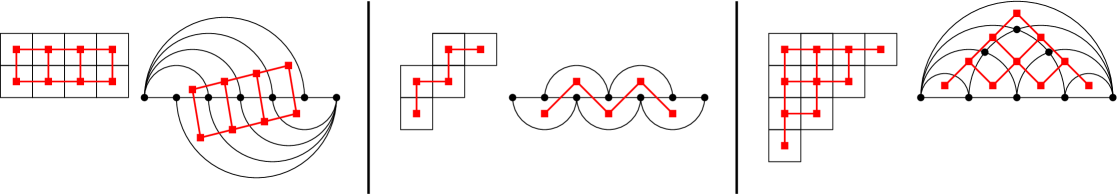
By Stanley’s theory of order polytopes [26] it follows that the volume of the polytope $P_{\lambda}(n)$ for any $P_{\lambda}(n)\in{\mathcal{F}}(ASM)(n)$ is given by the number of linear extensions of the poset $(\delta_{n}\setminus\lambda)^{*}$ (which equals the number of standard Young tableaux of skew shape $\delta_{n}/\lambda)$ , and its Ehrhart polynomial in the variable $t$ is given by the order polynomial of the poset $(\delta_{n}\setminus\lambda)^{*}$ . See Corollary 5.7 for the general statement. We give the application to ${\mathcal{ASMCRY}(n)}$ in the corollary below. For further examples of polytopes in ${\mathcal{F}}(ASM)(n)$ , see Figure 9.

Corollary 1.2.

${\mathcal{ASMCRY}(n)}$ is integrally equivalent to the order polytope of the poset $\delta_{n}^{*}$ . Thus, ${\mathcal{ASMCRY}(n)}$ has ${\rm Cat}(n)=\frac{1}{n+1}\binom{2n}{n}$ vertices, its normalized volume is given by

{\rm vol}({\mathcal{ASMCRY}(n)})=\#SYT(\delta_{n}),

and its Ehrhart polynomial is

(1.1)

L_{{\mathcal{ASMCRY}(n)}}(t)=\Omega_{\delta_{n}^{*}}(t+1)=\prod_{1\leq i<j\leq n}\frac{2t+i+j-1}{i+j-1}.

Also, since the CRY polytope is contained in the ASM-CRY polytope then the formulas above are upper bound for the volume and number of lattice points of the former polytope (Corollary 5.8).

In Theorems 3.11 and 3.14, we make explicit the relationship between flow and order polytopes, showing that they correspond under certain planarity conditions of the respective graph and poset. As an application we obtain flow polytopes with volume equal to the number of standard Young tableaux of any skew shape $\lambda/\mu$ (see Figure 7).

For the definitions of $(\delta_{n}\setminus\lambda)^{*}$ and $G_{(\delta_{n}\setminus\lambda)^{*}}$ , see Definition 5.4 and the discussion before Theorem 3.14, respectively.

As mentioned earlier, a canonical triangulation of order polytopes was given by Stanley [26], and two families of triangulations of flow polytopes were constructed by Postnikov and Stanley [21, 25] as well as Danilov, Karzanov and Koshevoy [9]. It is natural to understand the relation among these triangulations, and we prove the following results, the first of which was first observed by Postnikov [21]. For the necessary definitions, see Sections 6 and 7.

Theorem 1.3 (Postnikov [21]).

Given a planar graph $G$ , the canonical triangulation of the order polytope $\widehat{{\mathcal{O}}}(P_{G})$ maps to the Danilov-Karzanov-Koshevoy triangulation of ${\mathcal{F}}_{G}$ coming from the planar framing via the integral equivalence map $\phi:\widehat{{\mathcal{O}}}(P_{G})\rightarrow{\mathcal{F}}_{G}$ given in Theorem 3.14.

Theorem 1.4.

Given a framed graph $G$ , the set of Danilov-Karzanov-Koshevoy triangulations of the flow polytope ${\mathcal{F}}_{G}$ equals the set of framed Postnikov-Stanley triangulations of ${\mathcal{F}}_{G}$ .

All three of the above-mentioned triangulations are indexed by natural sets of combinatorial objects and we give explicit bijections between these sets in Sections 6 and 7.

The outline of the paper is as follows. In Section 2, we discuss the Birkhoff and alternating sign matrix polytopes, as well as some of their faces. In Sections 3 and 4 we give background information on flow and order polytopes and show that flow polytopes of planar graphs are order polytopes and that order polytopes of strongly planar posets are flow polytopes. In Section 5 we study a family of faces of the alternating sign matrix polytopes and show that they are integrally equivalent to both flow and order polytopes and calculate their volumes and Ehrhart polynomials in particularly nice cases. In Section 6, we study triangulations of flow polytopes of planar graphs (which include the polytopes of Section 5) and show that their canonical triangulations defined by Stanley [26] are also Danilov-Karzanov-Koshevoy triangulations [9]. Finally, in Section 7, we study the Danilov-Karzanov-Koshevoy triangulations and the framed Postnikov-Stanley triangulations of flow polytopes of an arbitrary graph. We show that these sets are equal. We also exhibit explicit bijections between the combinatorial objects indexing the various triangulations, answering a question raised by Postnikov [21].

2. Faces of the Birkhoff and alternating sign matrix polytopes

In this section, we explain the motivation for our study of certain faces of the alternating sign matrix polytope. We review some standard facts of lattice point enumeration of integral polytopes [4],[27, §4.6]. Given an integral polytope $\mathcal{P}$ , we denote by ${\rm relvol}(\mathcal{P})$ the volume of $\mathcal{P}$ relative to its lattice and by $L_{\mathcal{P}}(t)$ the Ehrhart function that counts the number of lattice points of the dilated polytope $t\cdot\mathcal{P}$ . A well known result of Ehrhart [11] states that if $\mathcal{P}$ is integral, then $L_{\mathcal{P}}(t)$ is a polynomial of degree $\dim(\mathcal{P})$ with leading coefficient ${\rm relvol}(\mathcal{P})$ (see [4, Cor. 3.16]). The quantity $\dim(\mathcal{P})!\cdot{\rm relvol}(\mathcal{P})$ is an integer (see [4, Cor. 3.17]) called the normalized volume that we denote by ${\rm vol}(\mathcal{P})$ .

We say that two integral polytopes $\mathcal{P}$ in $\mathbb{R}^{d}$ and $\mathcal{Q}$ in $\mathbb{R}^{m}$ are integrally equivalent, which we denote by $\mathcal{P}\overset{\mathrm{int}}{\equiv}\mathcal{Q}$ , if there is an affine transformation $\varphi:\mathbb{R}^{d}\to\mathbb{R}^{m}$ whose restriction to $\mathcal{P}$ is a bijection $\varphi:\mathcal{P}\to\mathcal{Q}$ that preserves the lattice, i.e. $\varphi$ is a bijection between $\mathbb{Z}^{d}\cap{\rm aff}(\mathcal{P})$ and $\mathbb{Z}^{m}\cap{\rm aff}(\mathcal{Q})$ where ${\rm aff}(\cdot)$ denotes the affine span. The map $\varphi$ is then an integral equivalence. Note that integrally equivalent polytopes have the same Ehrhart polynomials and therefore they have the same volume. We remark that isomorphism and unimodular equivalence are other terms sometimes used in the literature for what we will refer to as integral equivalence.

Next we define the Birkhoff and Chan-Robbins-Yuen polytopes; we then define the alternating sign matrix counterparts.

Definition 2.1.

The Birkhoff polytope, $\mathcal{B}(n)$ , is defined as

\mathcal{B}(n):={\Big{\{}}(b_{ij})_{i,j=1}^{n}\in\mathbb{R}^{n^{2}}\mid b_{ij}\geq 0,\,\,\,{\sum_{i}}b_{ij}=1,\,\,\,\sum_{j}b_{ij}=1{\Big{\}}}.

Matrices in $\mathcal{B}(n)$ are called doubly-stochastic matrices. A well-known theorem of Birkhoff [6] and von Neumann [30] states that $\mathcal{B}(n)$ , as defined above, equals the convex hull of the $n\times n$ permutation matrices. Note that $\mathcal{B}(n)$ has $n^{2}$ facets and dimension $(n-1)^{2}$ , its vertices are the permutation matrices, and its volume has been calculated up to $n=10$ by Beck and Pixton [3]. De Loera, Liu and Yoshida [10] gave a closed summation formula for the volume of $\mathcal{B}(n)$ , which, while of interest on its own right, does not lend itself to easy computation. Shortly after, Canfield and McKay [7] gave an asymptotic formula for the volume.

A special face of the Birkhoff polytope, first studied by Chan-Robbins-Yuen [8], is as follows.

Definition 2.2.

The Chan-Robbins-Yuen polytope, $\mathcal{CRY}(n)$ , is defined as

\mathcal{CRY}(n):=\left\{(b_{{i}{j}})_{i,j=1}^{n}\in\mathcal{B}(n)\mid b_{{i}{j}}=0\mbox{ for }i-j\geq 2\right\}.

$\mathcal{CRY}(n)$ has dimension $\binom{n}{2}$ and $2^{n-1}$ vertices. This polytope was introduced by Chan-Robbins-Yuen [8] and in [31] Zeilberger calculated its normalized volume as the following product of Catalan numbers.

Theorem 2.3 (Zeilberger [31]).

{\rm vol}(\mathcal{CRY}(n))=\prod_{i=1}^{n-2}{\rm Cat}(i)

where ${\rm Cat}(i)=\frac{1}{i+1}\binom{2i}{i}$ .

The proof in [31] used a relation (see Theorem 3.4) expressing the volume as a value of the Kostant partition function (see Definition 3.5) and a reformulation of the Morris constant term identity [20] to calculate this value. No combinatorial proof is known.

Next we give an analogue of the Birkhoff polytope in terms of alternating sign matrices. Recall that alternating sign matrices (ASMs) [17] are square matrices with the following properties:

•

entries $\in\{0,1,-1\}$ ,
•

the entries in each row/column sum to 1, and
•

the nonzero entries along each row/column alternate in sign.

The ASMs with no negative entries are the permutation matrices. See Figure 1 for an example.

$\left(\begin{array}[]{rrr}1&0&0\\ 0&1&0\\ 0&0&1\end{array}\right)\left(\begin{array}[]{rrr}1&0&0\\ 0&0&1\\ 0&1&0\end{array}\right)\left(\begin{array}[]{rrr}0&1&0\\ 1&0&0\\ 0&0&1\end{array}\right)\left(\begin{array}[]{rrr}0&1&0\\ 1&-1&1\\ 0&1&0\end{array}\right)\left(\begin{array}[]{rrr}0&1&0\\ 0&0&1\\ 1&0&0\end{array}\right)\left(\begin{array}[]{rrr}0&0&1\\ 1&0&0\\ 0&1&0\end{array}\right)\left(\begin{array}[]{rrr}0&0&1\\ 0&1&0\\ 1&0&0\end{array}\right)$

Figure 1. All the

3\times 3

alternating sign matrices.

Definition 2.4 (Behrend-Knight [5], Striker [29]).

The alternating sign matrix polytope, $\mathcal{A}(n)$ , is defined as follows:

\mathcal{A}(n):={\Big{\{}}(a_{ij})_{i,j=1}^{n}\in\mathbb{R}^{n^{2}}\mid 0\leq{\displaystyle\sum_{i=1}^{i^{\prime}}a_{ij}\leq 1,\,\,0\leq\displaystyle\sum_{j=1}^{j^{\prime}}a_{ij}\leq 1,\,\,\displaystyle\sum_{i=1}^{n}}a_{ij}=1,\,\,\displaystyle\sum_{j=1}^{n}a_{ij}=1{\Big{\}}},

where we have the first sum for any $1\leq i^{\prime},j\leq n$ , the second sum for any $1\leq j^{\prime},i\leq n$ , the third sum for any $1\leq j\leq n$ , and the fourth sum for any $1\leq i\leq n$ .

Behrend and Knight [5], and independently Striker [29], defined $\mathcal{A}(n)$ . The alternating sign matrix polytope can be seen as an analogue of the Birkhoff polytope, since the former is the convex hull of all alternating sign matrices (which include all permutation matrices) while the latter is the convex hull of all permutation matrices. The polytope $\mathcal{A}(n)$ has $4((n-2)^{2}+1)$ facets (for $n\geq 3$ ) [29], its dimension is $(n-1)^{2}$ , and its vertices are the $n\times n$ alternating sign matrices [5, 29]. The Ehrhart polynomial has been calculated up to $n=5$ [5]. Its normalized volume for $n=1,\ldots,5$ is calculated to be

1,1,4,1376,201675688,

and no asymptotic formula for its volume is known.

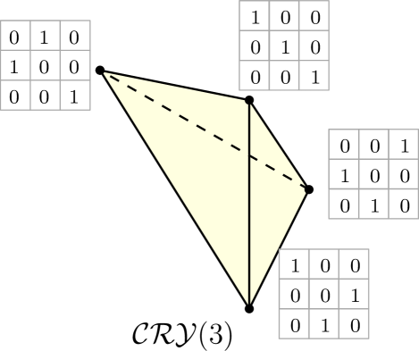
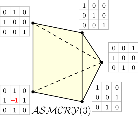
In analogy with ${\mathcal{CRY}}(n)$ , we study a special face of the ASM polytope we call the ASM-CRY polytope (and show, in Theorem 5.3, it is indeed a face of $\mathcal{A}(n)$ ).

Definition 2.5.

The ASM-CRY polytope is defined as follows.

{\mathcal{ASMCRY}(n)}:=\left\{(a_{{i}{j}})_{i,j=1}^{n}\in\mathcal{A}(n)\mid a_{{i}{j}}=0\mbox{ for }{i}-{j}\geq 2\right\}.

Since the ${\mathcal{CRY}}(n)$ polytope has a nice product formula for its normalized volume, it is then natural to wonder if the volume of the alternating sign matrix analogue of ${\mathcal{CRY}}(n)$ , which we denote by ${\mathcal{ASMCRY}(n)}$ , is similarly nice. In Theorem 1.1 and Corollary 1.2, we show that ${\mathcal{ASMCRY}(n)}$ is both a flow and order polytope, and using the theory established for the latter, we give the volume formula and the Ehrhart polynomial of ${\mathcal{ASMCRY}(n)}$ . Just like in the ${\mathcal{CRY}}(n)$ case, all formulas obtained are combinatorial. Unlike in the ${\mathcal{CRY}}(n)$ case, all the proofs involved are combinatorial. In Theorem 1.1, we extend these results to a family of faces ${\mathcal{F}}(ASM)(n)$ of the ASM polytope, of which ${\mathcal{ASMCRY}(n)}$ is a member; see Section 5.

Refer to caption — Figure 2. (a) The polytope $\mathcal{CRY}(3)$ in $\mathbb{R}^{3}$ , (b) the polytope $\mathcal{ASMCRY}(3)$ in $\mathbb{R}^{3}$ , (c) a doubly-stochastic matrix in $\mathcal{CRY}(4)$ , (d) a matrix in $\mathcal{ASMCRY}(4)$ .

3. Flow and order polytopes

In order to state and prove Theorem 1.1 in Section 5, we need to discuss flow and order polytopes. In Section 3.1, we define flow and order polytopes and also explain how to see ${\mathcal{CRY}}(n)$ as the flow polytope of the complete graph. In Sections 3.2 and 3.3, we state in Theorems 3.11 and 3.14 that the flow polytope of a planar graph is the order polytope of a related poset, and vice versa. We give the proofs of these theorems in Section 4.

3.1. Background and definitions

Let $G$ be a connected graph on the vertex set $[n]:=\{1,2,\ldots,n\}$ with edges directed from the smaller to larger vertex. Denote by ${\rm in}(e)$ the smaller (initial) vertex of edge $e$ and ${\rm fin}(e)$ the bigger (final) vertex of edge $e$ .

Definition 3.1.

Given a vector ${\bf a}=(a_{1},a_{2},\ldots,a_{n-1},-\sum_{i=1}^{n-1}a_{i})$ with $a_{i}\in\mathbb{Z}_{\geq 0}$ , a flow $fl$ on $G$ with netflow ${\bf a}$ is a function $fl:E(G)\rightarrow\mathbb{R}_{\geq 0}$ such that for $i=1,2,\ldots,n-1$

\sum_{e\in E,{\rm in}(e)=i}fl(e)\,-\,\sum_{e\in E,{\rm fin}(e)=i}fl(e)=a_{i}

and

\sum_{e\in E,{\rm fin}(e)=n}fl(e)=\sum_{i=1}^{n-1}a_{i}.

The flow polytope ${\mathcal{F}}_{G}({\bf a})$ associated to the graph $G$ and netflow vector ${\bf a}$ is the set of all flows $fl:E(G)\rightarrow\mathbb{R}_{\geq 0}$ on $G$ with netflow ${\bf a}$ . We denote the set of integer flows of ${\mathcal{F}}_{G}({\bf a})$ by ${\mathcal{F}}_{G}^{{\rm int}}({\bf a})$ .

Definition 3.2.

A flow $fl$ of size one on $G$ is a flow on $G$ with netflow $(1,0,\ldots,0,-1)$ . That is

\sum_{e\in E,{\rm in}(e)=1}fl(e)\,=\,\sum_{e\in E,{\rm fin}(e)=i}fl(e)\,=\,1,

and for $2\leq i\leq n-1$

\sum_{e\in E,{\rm fin}(e)=i}fl(e)\,=\,\sum_{e\in E,{\rm in}(e)=i}fl(e).

The flow polytope ${\mathcal{F}}_{G}$ associated to the graph $G$ is the set of all flows $fl:E(G)\rightarrow\mathbb{R}_{\geq 0}$ of size one on $G$ .

We assume that in our flow polytopes ${\mathcal{F}}_{G}$ each vertex $v\in\{2,3,\ldots,n-1\}$ in $G$ has both incoming and outgoing edges. Note that this restriction is not a serious one. If there is a vertex $v\in[2,n-1]$ with only incoming or outgoing edges, then in ${\mathcal{F}}_{G}$ the flow on all these edges must be zero, and thus, up to removing such vertices, any flow polytope ${\mathcal{F}}_{G}$ is integrally equivalent to a flow polytope defined as above.

The polytope ${\mathcal{F}}_{G}$ is a convex polytope in the Euclidean space $\mathbb{R}^{\#E(G)}$ and its dimension is $\dim({\mathcal{F}}_{G})=\#E(G)-\#V(G)+1$ (e.g. see [1]). The vertices of ${\mathcal{F}}_{G}$ are characterized as follows.

Proposition 3.3 ([13, Cor. 3.1]).

Let $G$ be a connected graph with vertices $[n]$ with edges oriented from smaller to bigger vertices. Then the vertices of ${\mathcal{F}}_{G}$ are the unit flows on maximal directed paths or routes from the source $1$ to the sink $n$ .

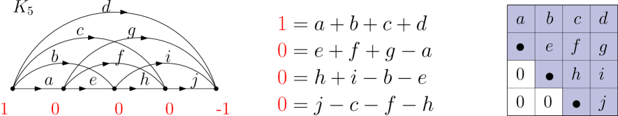
Figure 3 shows the equations of ${\mathcal{F}}_{K_{5}}$ and explains why this polytope is integrally equivalent to ${\mathcal{CRY}}(4)$ . The same correspondence shows that ${\mathcal{F}}_{K_{n+1}}$ and ${\mathcal{CRY}}(n)$ coincide. The following theorem connects volumes of flow polytopes and Kostant partition functions.

Theorem 3.4 (Postnikov-Stanley [21, 25], Baldoni-Vergne [1]).

For a loopless graph $G$ on the vertex set $\{1,2\ldots,n\}$ , with $d_{i}=indeg_{i}(G)-1$ ,

{\rm vol}\left({\mathcal{F}}_{G}\right)=K_{G}(0,d_{2},\ldots,d_{n-1},-\sum_{i=2}^{n-1}d_{i}),

where $K_{G}({\bf a})$ is the Kostant partition function, $indeg_{i}(G)$ denotes the indegree of vertex $i$ in $G$ and ${\rm vol}$ is normalized volume.

Recall the definition of the Kostant partition function.

Definition 3.5.

The Kostant partition function $K_{G}({\rm v})$ is the number of ways to write the vector ${\rm v}$ as a nonnegative linear combination of the positive type $A_{n-1}$ roots corresponding to the edges of $G$ , without regard to order. The edge $(i,j)$ , $i<j$ , of $G$ corresponds to the vector $e_{i}-e_{j}$ , where $e_{i}$ is the $i^{th}$ standard basis vector in $\mathbb{R}^{n}$ .

It is easy to see by definition that the number of integer flows on $G$ with netflow ${\bf a}$ , that is, the size of ${\mathcal{F}}_{G}^{{\rm int}}({\bf a})$ or number of integer points in the flow polytope ${\mathcal{F}}_{G}({\bf a})$ , equals $K_{G}({\bf a})$ . In particular, the Ehrhart polynomial of ${\mathcal{F}}_{G}$ in variable $t$ is equal to $K_{G}(t,0,\ldots,0,-t).$

Now we are ready to define order polytopes and relate them to flow polytopes.

Definition 3.6 (Stanley [26]).

The order polytope, $\mathcal{O}(P)$ , of a poset $P$ with elements $\{t_{1},t_{2},\ldots,t_{n}\}$ is the set of points $(x_{1},x_{2},\ldots,x_{n})$ in $\mathbb{R}^{n}$ with $0\leq x_{i}\leq 1$ and if $t_{i}\leq_{P}t_{j}$ then $x_{i}\leq x_{j}$ . We identify each point $(x_{1},x_{2},\ldots,x_{n})$ of $\mathcal{O}(P)$ with the function $f:P\to\mathbb{R}$ with $f(t_{i})=x_{i}$ .

In our proofs, we will often use the polytope $\hat{\mathcal{O}}(P)$ , which is integrally equivalent to $\mathcal{O}(P)$ [26, Sec. 1]:

Definition 3.7 (Stanley [26]).

Let $\widehat{P}$ be the poset obtained from $P$ by adjoining a minimum element $\hat{0}$ and a maximum element $\hat{1}$ . Define a polytope $\widehat{\mathcal{O}}(P)$ to be the set of functions $g:\widehat{P}\to\mathbb{R}$ satisfying $g(\hat{0})=0$ , $g(\hat{1})=1$ , and $g(x)\leq g(y)$ if $x\leq y$ in $\widehat{P}$ .

Lemma 3.8 (Stanley [26]).

The map $\nu:\widehat{\mathcal{O}}(P)\to\mathcal{O}(P)$ given by $(g(x))_{x\in\widehat{P}}\mapsto(g(x))_{x\in{P}}$ is an integral equivalence.

In general, computing or finding a combinatorial interpretation for the volume of a polytope is a hard problem. Order polytopes are an especially nice class of polytopes whose volume has a combinatorial interpretation.

Theorem 3.9 (Stanley [26]).

Given a poset $P$ we have that

(i)

the vertices of $\mathcal{O}(P)$ are in bijection with characteristic functions of complements of order ideals of $P$ ,
(ii)

the normalized volume of $\mathcal{O}(P)$ is $e(P)$ , where $e(P)$ is the number of linear extensions of $P$ ,
(iii)

the Ehrhart polynomial $L_{\mathcal{O}(P)}(m)$ of $\mathcal{O}(P)$ equals the order polynomial $\Omega(P,m+1)$ of $P$ .

Definition 3.10.

Given a poset $P$ and a positive integer $m$ , the order polynomial $\Omega(P,m)$ is the number of order preserving maps $\eta:P\rightarrow\left\{1,2,\ldots,m\right\}$ .

3.2. Flow polytopes of planar graphs are order polytopes

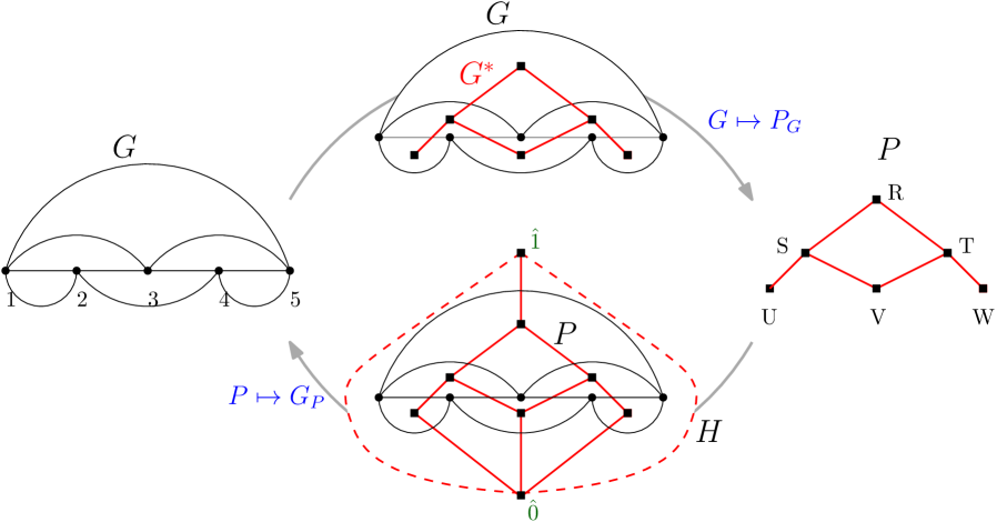
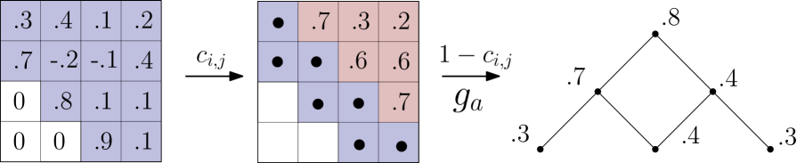
The following theorem, which states that a flow polytope of a planar graph is an order polytope, is a result communicated to us by Postnikov [21]. Given a connected graph $G$ with the conventions of Section 3.1, we say that $G$ is planar if it has a planar embedding so that if vertex $i$ is in position $(x_{i},y_{i})$ then $x_{i}<x_{j}$ whenever $i<j$ . We denote by $G^{*}$ the truncated dual graph of $G$ , which is the dual graph with the vertex corresponding to the infinite face deleted. The orientation of the edges of $G$ induces an orientation of the edges of $G^{*}$ (faces of $G$ ) from lower to higher $y$ -coordinates of the end points. This allows us to consider $G^{*}$ as the Hasse diagram of a poset that we denote by $P_{G}$ . See Figure 4. Note that by Euler’s formula, $\#P_{G}=\#E(G)-\#V(G)+1$ which equals $\dim(\mathcal{F}_{G})$ . Let $\widehat{P}_{G}:=P_{G}\sqcup\{\hat{0},\hat{1}\}$ .

Theorem 3.11 (Postnikov [21]).

Let $G$ be a planar graph on the vertex set $[n]$ such that at each vertex $v\in[2,n-1]$ there are both incoming and outgoing edges. Fix a planar embedding of $G$ with the above conventions. Then the map $\varphi:\mathcal{F}_{G}\to\widehat{\mathcal{O}}(P_{G})$ given in Definition 3.12 is an integral equivalence. In particular, $\mathcal{F}_{G}\overset{\mathrm{int}}{\equiv}\widehat{\mathcal{O}}(P_{G})\overset{\mathrm{int}}{\equiv}\mathcal{O}(P_{G})$ .

Definition 3.12.

Define $\varphi:\mathcal{F}_{G}\to\widehat{\mathcal{O}}(P_{G})$ by $fl\mapsto(f(x))_{x\in P_{G}}$ , where $f:\widehat{P}_{G}\to\mathbb{R}_{\geq 0}$ is given by

(3.1)

f(x)=\sum_{e\in\mathsf{p}}fl(e).

The latter sum is taken over the edges $e$ that are intersected by a(ny) path $\mathsf{p}$ in $\widehat{P}_{G}$ from $\hat{0}$ to $x$ .

Example 3.13.

Given the graph $G$ and the corresponding poset $P_{G}$ in Figure 5, the map $fl\mapsto f$ from Definition 3.12 is as follows:

	$\displaystyle f(R)$	$\displaystyle=fl(b)+fl(c)+fl(d),$
	$\displaystyle f(S)$	$\displaystyle=fl(c)+fl(d)$
	$\displaystyle f(T)$	$\displaystyle=fl(i)+fl(j)$
	$\displaystyle f(U)$	$\displaystyle=fl(d)$
	$\displaystyle f(V)$	$\displaystyle=fl(f)$
	$\displaystyle f(W)$	$\displaystyle=fl(j).$

Lemma 4.1 below shows that $f$ in Definition 3.12 is well-defined, while Lemma 4.2 shows that $\varphi$ indeed maps points in ${\mathcal{F}}_{G}$ to points in $\widehat{\mathcal{O}}({P}_{G})$ . The proof of Theorem 3.11 is given in Section 4.

3.3. Order polytopes of strongly planar posets are flow polytopes

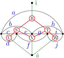
We now state a converse of Theorem 3.11, showing that the order polytope of a strongly planar poset is a flow polytope. A poset $P$ is strongly planar if the Hasse diagram of $\widehat{P}:=P\sqcup\{\hat{0},\hat{1}\}$ has a planar embedding with $y$ coordinates respecting the order of the poset. For example, the “bowtie” poset defined by the relations $a<c,a<d,b<c,b<d$ is planar, but not strongly planar. Given a strongly planar poset $P$ , let $H$ be the (planar) graph obtained from the Hasse diagram of $\widehat{P}$ with two additional edges from $\widehat{0}$ to $\widehat{1}$ , one of which goes to the left of all the poset elements and another to the right. We can then define the graph $G_{P}$ to be the truncated dual of $H$ . The orientation of $G_{P}$ is inherited from the poset in the following way: if in the construction of the truncated dual, the edge $e$ of $G_{P}$ crosses the edge $x\rightarrow y$ where $x<y$ in $P$ , then $y$ is on the left and $x$ is on the right as you traverse $e$ . See Figure 4.

Theorem 3.14.

If $P$ is a strongly planar poset, then the map $\phi:\widehat{\mathcal{O}}(P)\to\mathcal{F}_{G_{P}}$ given in Definition 3.15 is an integral equivalence. In particular, $\mathcal{O}(P)\overset{\mathrm{int}}{\equiv}\widehat{\mathcal{O}}(P)\overset{\mathrm{int}}{\equiv}\mathcal{F}_{G_{P}}$ .

Definition 3.15.

Define $\phi:\widehat{\mathcal{O}}(P)\to\mathcal{F}_{G_{P}}$ by $(f(x))_{x\in\hat{P}}\mapsto fl$ , where $fl:E(G_{P})\to\mathbb{R}_{\geq 0}$ is given by

(3.2)

fl(e)=f(y)-f(x),

where $e$ crosses the Hasse diagram edge $x\rightarrow y$ (in the dual construction).

Example 3.16.

Given the graph $G$ and the corresponding poset $P_{G}$ in Figure 5, the map $f\mapsto fl$ from Definition 3.15 is as follows:

	$\displaystyle fl(a)$	$\displaystyle=1-f(R)$
	$\displaystyle fl(b)$	$\displaystyle=f(R)-f(S)$
	$\displaystyle fl(c)$	$\displaystyle=f(S)-f(U)$
	$\displaystyle fl(d)$	$\displaystyle=f(U)$
	$\displaystyle fl(e)$	$\displaystyle=f(S)-f(V)$

	$\displaystyle fl(f)$	$\displaystyle=f(V)$
	$\displaystyle fl(g)$	$\displaystyle=f(T)-f(V)$
	$\displaystyle fl(h)$	$\displaystyle=f(R)-f(T)$
	$\displaystyle fl(i)$	$\displaystyle=f(T)-f(W)$
	$\displaystyle fl(j)$	$\displaystyle=f(W).$

We postpone the proof of Theorem 3.14 result to Section 4.

4. Proofs of Theorem 3.11 and Theorem 3.14

This section provides the proofs of Theorems 3.11 and 3.14.

Lemma 4.1.

Given a flow $fl\in{\mathcal{F}}_{G}$ , the map $f:\widehat{P}_{G}\to\mathbb{R}_{\geq 0}$ is independent on the path $\mathsf{p}$ chosen in (3.1).

Proof.

Let $\mathsf{p}_{1}$ and $\mathsf{p}_{2}$ be two paths in $\widehat{P}_{G}$ from $\hat{0}$ to $x$ . We show that

(4.1)

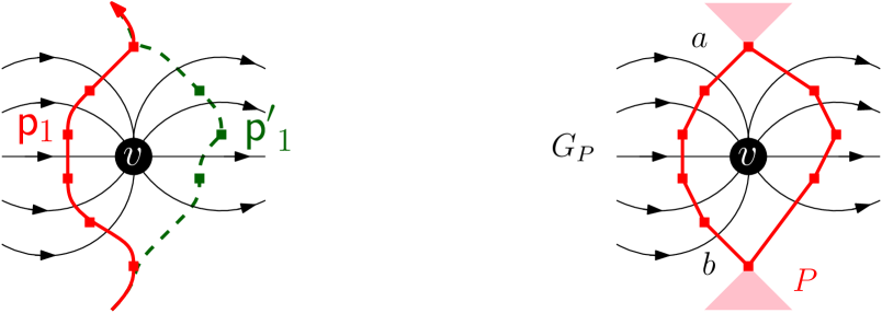
\sum_{e\in\mathsf{p}_{1}}fl(e)=\sum_{e\in\mathsf{p}_{2}}fl(e).

If $\mathsf{p}_{1}$ and $\mathsf{p}_{2}$ coincide, (4.1) is trivial. We induct on the number of vertices of $G$ enclosed by the two paths $\mathsf{p}_{1}$ and $\mathsf{p}_{2}$ . Without loss of generality, assume $\mathsf{p}_{1}$ is left of $\mathsf{p}_{2}$ given the planar drawing of $G$ . Let $v$ be the vertex with the smallest $x$ -coordinate enclosed by the two paths $\mathsf{p}_{1}$ and $\mathsf{p}_{2}$ in the planar drawing of $G$ . By construction, all the incoming edges in $G$ to $v$ are crossed by path $\mathsf{p}_{1}$ and $x$ is not a face between two incoming edges to $v$ . Next, we do the following local move to change the path $\mathsf{p}_{1}$ : let $\mathsf{p}^{\prime}_{1}$ be the path that coincides with $\mathsf{p}_{1}$ except that it crosses the outgoing edges of $v$ (see Figure 6). By conservation of flow on vertex $v$ , the sum of the flow of the incoming edges to $v$ equals the sum of the flow of the outgoing edges from $v$ . Since these are the only crossed edges that $\mathsf{p}_{1}$ and $\mathsf{p}^{\prime}_{1}$ differ on we have that

\sum_{e\in\mathsf{p}_{1}}fl(e)=\sum_{e\in\mathsf{p}^{\prime}_{1}}fl(e).

The paths $\mathsf{p}^{\prime}_{1}$ and $\mathsf{p}_{2}$ have one fewer vertex of $G$ enclosed by them than the paths $\mathsf{p}_{1}$ and $\mathsf{p}_{2}$ . By induction we have

\sum_{e\in\mathsf{p}^{\prime}_{1}}fl(e)=\sum_{e\in\mathsf{p}_{2}}fl(e).

Comparing the latter two equations, the result follows. ∎

Next, we show that given a flow $fl$ in ${\mathcal{F}}_{G}$ the point $\varphi(fl)=(f(x))_{x\in P_{G}}$ is in $\widehat{\mathcal{O}}(P_{G})$ .

Lemma 4.2.

Given a flow $fl\in{\mathcal{F}}_{G}$ , the image $\varphi(fl)\in\widehat{\mathcal{O}}(P_{G})$ .

Proof.

Note that $f(\hat{0})=0$ . We have that $0\leq f(x)$ since $fl(e)\geq 0$ for all edges $e$ . Also, $f(x)\leq 1$ since the set of edges whose sum of flows equals $f(x)$ can always be extended to a path from $\hat{0}$ to $\hat{1}$ . By repeated application of Lemma 4.1, the total flow in such a path is $1$ . Thus, $f(\hat{1})=1$ . Next, if $x^{\prime}$ covers $x$ in $\widehat{P}_{G}$ then there is an edge $e^{\prime}$ in $G$ separating the graph faces $x$ and $x^{\prime}$ . Thus $f(x^{\prime})=fl(e^{\prime})+f(x)\geq f(x)$ . Hence the linear map $f$ takes a point $(fl(e))_{e\in E(G)}$ of ${\mathcal{F}}_{G}$ to the point $(f(x))_{x\in P_{G}}$ of the order polytope $\widehat{\mathcal{O}}(P_{G})$ . ∎

Lemma 4.3.

Given a point in $\widehat{\mathcal{O}}(P)$ viewed as a function $f:\widehat{P}\to\mathbb{R}_{\geq 0}$ , the flow $fl:E(G_{P})\to\mathbb{R}_{\geq 0}$ as in Definition 3.15 is in $\mathcal{F}_{G_{P}}$ .

Proof.

Let $f:\widehat{P}\to\mathbb{R}_{\geq 0}$ be a point in $\widehat{\mathcal{O}}(P)$ and let $e$ be an edge in $G_{P}$ crossing the Hasse diagram edge $x\rightarrow y$ of $\widehat{P}$ . Since $x\leq_{P}y$ then by definition of $\widehat{\mathcal{O}}(P)$ , $fl(e)=f(y)-f(x)\geq 0$ .

Next, we find the netflows at each vertex of $G$ . Consider the leftmost (rightmost) path in $\widehat{P}$ from $\hat{0}$ to $\hat{1}$ . This path crosses all the outgoing (incoming) edges in $G$ of vertex $1$ (vertex $n$ ). We have that

\sum_{e\in E,{\rm in}(e)=1}fl(e)=\sum_{e\in E,{\rm fin}(e)=n}fl(e)=f(\hat{1})-f(\hat{0})=1-0=1.

For an internal vertex $v\in[2,n-1]$ , let $a$ be the face bordering the highest incoming and outgoing edge to $v$ . Similarly, let $b$ be the face bordering the lowest incoming and outgoing edge to $v$ . Consider the paths $\mathsf{p}_{in}$ and $\mathsf{p}_{out}$ be the paths in $\widehat{P}$ from $b$ to $a$ crossing the incoming and outgoing edges to $v$ respectively (see Figure 6, Right). Then the total incoming and outgoing flow to vertex $v$ are

	$\displaystyle\sum_{e\in E,{\rm fin}(e)=v}fl(e)$	$\displaystyle=\sum_{z\to w\text{ in }\mathsf{p}_{in}}(f(w)-f(z))=f(a)-f(b),$
	$\displaystyle\sum_{e\in E,{\rm in}(e)=v}fl(e)$	$\displaystyle=\sum_{z\to w\text{ in }\mathsf{p}_{out}}(f(w)-f(z))=f(a)-f(b),$

This shows the flow is conserved on vertex $v$ , and thus $fl(\cdot)$ is in $\mathcal{F}_{G_{P}}$ . ∎

Lemma 4.3 shows that $\phi(\widehat{\mathcal{O}}(P))\subset\mathcal{F}_{G_{P}}$ .

Proof of Theorem 3.11 and Theorem 3.14.

Note that given a planar graph $G$ we have that $Q:=P_{G}$ is a strongly planar poset and that $G_{Q}=G$ . Given a flow $fl$ in ${\mathcal{F}}_{G}$ , let $f=\varphi(fl)$ the corresponding point in $\widehat{O}(P_{G})$ and $fl^{\prime}$ be the flow $\phi(\varphi(fl))=\phi(f)$ . Let $e$ be an edge of $G$ crossing the Hasse diagram edge $x\to y$ in $\widehat{P}_{G}$

	$\displaystyle fl^{\prime}(e)$	$\displaystyle=f(y)-f(x)$
		$\displaystyle=\sum_{e_{1}\in\mathsf{p}}fl(e_{1})-\sum_{e_{2}\in\mathsf{q}}fl(e_{2}),$

where $\mathsf{p}$ is a path $\widehat{P}_{G}$ from $\hat{0}$ to $y$ and $\mathsf{q}$ is a path $\widehat{P}_{G}$ from $\hat{0}$ to $x$ . By Lemma 4.1 the value of $f(y)$ is independent of the choice of path, so by letting $\mathsf{p}=\mathsf{q}+x\to y$ the last difference becomes $fl(e)$ , showing that $fl^{\prime}(e)=fl(e)$ . A similar argument shows that $\varphi\circ\phi$ is the identity. Thus the maps $\phi$ and $\varphi$ are inverses of each other and they both preserve integer points. Therefore, $\phi$ and $\varphi$ are integral equivalences. Using Lemma 3.8 giving $\widehat{\mathcal{O}}(P)\overset{\mathrm{int}}{\equiv}\mathcal{O}(P)$ for any poset $P$ we are done. ∎

Remark 4.4.

By Theorem 3.11, if $G$ is a planar graph then ${\mathcal{F}}_{G}$ is integrally equivalent to an order polytope. This raises the question of whether this relation holds for non-planar graphs: for instance for the polytope ${\mathcal{CRY}}(n)\cong{\mathcal{F}}_{K_{n+1}}$ for $n\geq 4$ . We can use a similar construction to that in the proof of Theorem 3.11 to show that ${\mathcal{F}}_{K_{5}}$ and ${\mathcal{F}}_{K_{6}}$ are integrally equivalent to the order polytopes of the posets:

We leave it as a question whether ${\mathcal{F}}_{K_{7}}$ (dimension $15$ , $32$ vertices, volume $140$ ) is an order polytope.

5. ${\mathcal{ASMCRY}(n)}$ and the family of polytopes ${\mathcal{F}}(ASM)$

In this section, we introduce the ASM-CRY family of polytopes ${\mathcal{F}}(ASM)$ , which includes ${\mathcal{ASMCRY}(n)}$ , and show that each of these polytopes is a face of the ASM polytope. We, furthermore, show that each polytope in this family is both an order and a flow polytope. Then, using the theory of order polytopes as discussed in Section 3.1, we determine their volumes and Ehrhart polynomials.

Definition 5.1.

Let $\delta_{n}=(n-1,n-2,\ldots,2,1)$ be the staircase partition considered as the positions $(i,j)$ of an $n\times n$ matrix given by $\left\{(i,j)\mid{j}-{i}\geq 1\right\}$ . Let the partition $\lambda=(\lambda_{1},\lambda_{2},\ldots,\lambda_{k})\subseteq\delta_{n}$ denote matrix positions $\left\{(i,j)\mid 1\leq i\leq k,\,\,n-\lambda_{i}+1\leq j\leq n,\,\,\lambda_{i}\leq n-i\right\}$ .

We define the ASM-CRY family

{\mathcal{F}}(ASM)(n):=\left\{\mathcal{P}_{\lambda}(n)\mid\lambda\subseteq\delta_{n}\right\},

where

\mathcal{P}_{\lambda}(n):=\left\{(a_{{i}{j}})_{i,j=1}^{n}\in\mathcal{A}(n)\mid a_{{i}{j}}=0\mbox{ for }{i}-{j}\geq 2\mbox{ and for }(i,j)\in\lambda\right\}.

Note that $\mathcal{P}_{\varnothing}(n)={\mathcal{ASMCRY}(n)}$ , as in Definition 2.5.

In the following proposition we give a convex hull description of the polytopes in this family.

Proposition 5.2.

The polytope ${\mathcal{P}}_{\lambda}(n)\in{\mathcal{F}}(ASM)(n)$ is the convex hull of the $n\times n$ alternating sign matrices $(A_{ij})_{i,j=1}^{n}$ with $A_{{i}{j}}=0\mbox{ for }{i}-{j}\geq 2\mbox{ and for }(i,j)\in\lambda$ .

Proof.

Let $\mathcal{Q}_{\lambda}(n)$ denote the convex hull of the $n\times n$ alternating sign matrices $(A_{ij})_{i,j=1}^{n}$ with $A_{{i}{j}}=0\mbox{ for }{i}-{j}\geq 2\mbox{ and for }(i,j)\in\lambda$ . It is easy to see that $\mathcal{Q}_{\lambda}(n)$ is contained in $\mathcal{P}_{\lambda}(n)$ , since matrices in both polytopes have the same prescribed zeros and satisfy the inequality description of the full ASM polytope $\mathcal{A}(n)$ .

It remains to prove that $\mathcal{P}_{\lambda}(n)$ is contained in $\mathcal{Q}_{\lambda}(n)$ . Suppose there exists a matrix $b=(b_{ij})_{i,j=1}^{n}\in{\mathcal{P}}_{\lambda}(n)$ such that $b\notin\mathcal{Q}_{\lambda}(n)$ . We know that $b$ is in the convex hull of all $n\times n$ ASMs. So $b=\mu_{1}A^{1}+\mu_{2}A^{2}+\cdots+\mu_{k}A^{k}$ , where $A^{1},\ldots A^{k}$ are distinct $n\times n$ alternating sign matrices and $\mu_{1},\ldots,\mu_{k}>0$ . At least one of these ASMs, say $A^{1}$ must have a nonzero entry $A^{1}_{ij}$ for some $(i,j)$ satisfying either ${i}-{j}\geq 2\mbox{ or }(i,j)\in\lambda$ . Suppose ${i}-{j}\geq 2$ ; the argument follows similarly in the case $(i,j)\in\lambda$ . Now since $b_{ij}=0$ and $A^{1}_{ij}\neq 0$ , there must be another ASM, say $A^{2}$ such that $A^{2}_{ij}$ is nonzero of opposite sign. Say $A^{1}_{ij}=1$ and $A^{2}_{ij}=-1$ . Then by the definition of an alternating sign matrix, there must be $j^{\prime}<j$ such that $A^{2}_{ij^{\prime}}=1$ . But $b_{ij^{\prime}}=0$ as well, so there must be an $A^{3}$ with $A^{3}_{ij^{\prime}}=-1$ and $j^{\prime\prime}<j^{\prime}$ such that $A^{3}_{ij^{\prime\prime}}=1$ . Eventually, we will reach the border of the matrix and reach a contradiction. 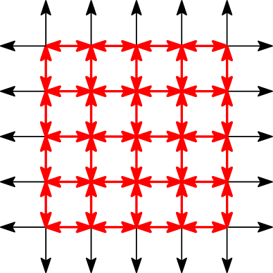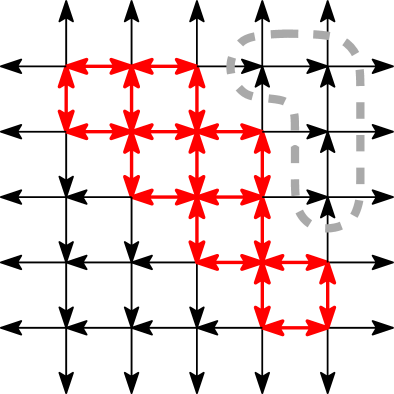Thus, $\mathcal{P}_{\lambda}(n)=\mathcal{Q}_{\lambda}(n)$ . ∎

We show in Theorem 5.3 below that the polytopes in ${\mathcal{F}}(ASM)(n)$ are faces of $\mathcal{A}(n)$ . First, we need some terminology from [29]. Consider $n^{2}+4n$ vertices on a square grid: $n^{2}$ ‘internal’ vertices $(i,j)$ and $4n$ ‘boundary’ vertices $(i,0)$ , $(0,j)$ , $(i,n+1)$ , and $(n+1,j)$ , where $1\leq i,j\leq n$ . Fix the orientation of this grid so that the first coordinate increases from top to bottom and the second coordinate increases from left to right, as in a matrix. The complete flow grid $C_{n}$ is defined as the directed graph on these vertices with directed edges pointing in both directions between neighboring internal vertices within the grid, and also directed edges from internal vertices to neighboring border vertices. That is, $C_{n}$ has edge set $\{((i,j),(i,j\pm 1)),((i,j),(i\pm 1,j))\mid i,j=1,\ldots,n\}$ . A simple flow grid of order $n$ is a subgraph of $C_{n}$ consisting of all the vertices of $C_{n}$ , and in which four edges are incident to each internal vertex: either four edges directed inward, four edges directed outward, or two horizontal edges pointing in the same direction and two vertical edges pointing in the same direction. An elementary flow grid is a subgraph of $C_{n}$ whose edge set is the union of the edge sets of some simple flow grids. See Figure 8.

Theorem 5.3.

The polytope ${\mathcal{P}}_{\lambda}(n)\in{\mathcal{F}}(ASM)(n)$ is a face of $\mathcal{A}(n)$ , of dimension $\binom{n}{2}-|\lambda|$ . In particular, ${\mathcal{P}}_{\varnothing}(n)={\mathcal{ASMCRY}(n)}$ is a face of $\mathcal{A}(n)$ , of dimension $\binom{n}{2}$ .

Proof.

In Proposition 4.2 of [29], it was shown that the simple flow grids of order $n$ are in bijection with the $n\times n$ alternating sign matrices. In this bijection, the internal vertices of the simple flow grid correspond to the ASM entries; the sources correspond to the ones of the ASM, the sinks correspond to the negative ones, and all other vertex configurations correspond to zeros. In Theorem 4.3 of [29], it was shown that the faces of $\mathcal{A}(n)$ are in bijection with $n\times n$ elementary flow grids, with the complete flow grid $C_{n}$ in bijection with the full ASM polytope $\mathcal{A}(n)$ . This bijection was given by noting that the convex hull of the ASMs in bijection with all the simple flow grids contained in an elementary flow grid is, in fact, an intersection of facets of the ASM polytope $\mathcal{A}(n)$ , and is thus a face of $\mathcal{A}(n)$ . Since, by Proposition 5.2, ${\mathcal{P}}_{\lambda}(n)$ equals the convex hull of the ASMs in it, we need only show there exists an elementary flow grid whose contained simple flow grids correspond exactly to these ASMs.

We can give this elementary flow grid explicitly. We claim that the directed edge set $S:=\bigcup_{(i,j)}S_{i,j}$ where

S_{i,j}:=\begin{cases}\left\{\left((i,j),(i,j-1)\right),\left((i,j),(i+1,j)\right)\right\}&\text{ if }i-j\geq 2\\ \left\{\left((i,j),(i,j+1)\right),\left((i,j),(i-1,j)\right)\right\}&\text{ if }(i,j)\in\lambda\\ \left\{\left((i,j),(i,j\pm 1)\right),\left((i,j),(i\pm 1,j)\right)\right\}&\text{ otherwise}\end{cases}

is the union of the directed edge sets of all the simple flow grids in bijection with ASMs in ${\mathcal{P}}_{\lambda}(n)$ . It is clear that the directed edge set of any simple flow grid corresponding to an ASM in ${\mathcal{P}}_{\lambda}(n)$ is in $S$ ; it remains to show that any edge in $S$ appears in some simple flow grid. Note that the directed edges listed in the first two cases appear in every simple flow grid in bijection with an ASM in ${\mathcal{P}}_{\lambda}(n)$ . For the remaining edges, note that if $A_{ij}=1$ , then in the corresponding simple flow grid, $S_{i,j}=\left\{\left((i,j),(i,j\pm 1)\right),\left((i,j),(i\pm 1,j)\right)\right\}$ . It is easy to construct a permutation matrix $A\in{\mathcal{P}}_{\lambda}(n)$ with $A_{ij}=1$ for any fixed $(i,j)$ with $i-j<2$ and $(i,j)\notin\lambda$ . Thus the digraph with the edge set $S$ is an elementary flow grid. Furthermore, no other simple flow grid can be constructed from directed edges in this set, since such a simple flow grid would have to include an edge pointing in the wrong direction in either the region ${i}-{j}\geq 2$ or $(i,j)\in\lambda$ . Thus, ${\mathcal{P}}_{\lambda}(n)$ is a face of $\mathcal{A}(n)$ .

To calculate the dimension of ${\mathcal{P}}_{\lambda}(n)$ , we use the following notion from [29]. A doubly directed region of an elementary flow grid is a connected collection of cells in the grid completely bounded by double directed edges but containing no double directed edges in the interior. Theorem 4.5 of [29] states that the dimension of a face of $\mathcal{A}(n)$ equals the number of doubly directed regions in the corresponding elementary flow grid. The number of doubly directed regions in the elementary flow grid corresponding to ${\mathcal{P}}_{\lambda}(n)$ equals $(n-1)^{2}-\left(\binom{n-1}{2}+|\lambda|\right)=\binom{n}{2}-|\lambda|$ . See Figure 8. ∎

Our main result regarding ${\mathcal{F}}(ASM)(n)$ is Theorem 1.1, which we prove below. It requires the following definition (see Figure 9 for examples); also, recall from Section 3.3 the definition of $G_{P}$ .

Definition 5.4.

Let $\delta_{n}$ and $\lambda\subseteq\delta_{n}$ be as in Definition 5.1. Let $(\delta_{n}\setminus\lambda)^{*}$ be the poset with elements $p_{ij}$ corresponding to the positions $(i,j)\in\delta_{n}\setminus\lambda$ with partial order $p_{ij}\leq p_{i^{\prime}j^{\prime}}$ if $i\geq i^{\prime}$ and $j\leq j^{\prime}$ .

We now prove Theorem 1.1 by first establishing two lemmas to show that $\mathcal{P}_{\lambda}(n)$ is integrally equivalent to the order polytope of the poset $(\delta_{n}\setminus\lambda)^{*}$ . Then since this poset is strongly planar, by Theorem 3.14 its order polytope is integrally equivalent to the flow polytope ${\mathcal{F}}_{G_{(\delta_{n}\setminus\lambda)^{*}}}$ .

Given a matrix $\left(a_{ij}\right)_{i,j=1}^{n}\in{\mathcal{P}}_{\lambda}(n)$ , define the corner sum matrix $\left(c_{ij}\right)_{i,j=1}^{n}$ by

c_{ij}=\displaystyle\sum_{\begin{subarray}{c}1\leq i^{\prime}\leq i,\\ j\leq j^{\prime}\leq n\end{subarray}}a_{i^{\prime}j^{\prime}}.

For $S\subseteq\mathbb{R}$ , let $\mathcal{A}(\delta_{n}\setminus\lambda,S)$ be the set of functions $g:\delta_{n}\setminus\lambda\to S$ . We view the order polytope of $(\delta_{n}\setminus\lambda)^{*}$ as a subset of $\mathcal{A}(\delta_{n}\setminus\lambda,[0,1])$ . Define $\Psi:\mathcal{P}_{\lambda}(n)\to\mathcal{A}(\delta_{n}\setminus\lambda,\mathbb{R})$ by $a\mapsto g_{a}$ where $g_{a}(i,j)=1-c_{ij}$ . See the second map in Figure 10.

Lemma 5.5.

The image of $\Psi$ is in $\mathcal{A}(\delta_{n}\setminus\lambda,[0,1])$ , i.e. if $a\mapsto g_{a}$ then $g_{a}(i,j)=1-c_{ij}\in[0,1]$ .

Proof.

We first show that $c_{ij}\geq 0$ for all $i$ and $j$ . By the defining inequalities of the ASM polytope $\mathcal{A}(n)$ (see Definition 2.4), we have that the partial row and column sums of any $a\in\mathcal{A}(n)$ satisfy the following for each fixed $1\leq i,j\leq n$ :

(5.1)

\sum_{i^{\prime}=1}^{i}a_{i^{\prime}j}\geq 0\text{ and }\sum_{j^{\prime}=j}^{n}a_{ij^{\prime}}\geq 0.

Since $c_{ij}=\sum_{i^{\prime}=1}^{i}\sum_{j^{\prime}=j}^{n}a_{i^{\prime}j^{\prime}}$ and the interior sum is nonnegative by (5.1), $c_{ij}\geq 0$ as desired.

Next we show that for $a\in{\mathcal{P}}_{\lambda}(n)$ , $c_{ij}\leq 1$ for all $j>i\geq 1$ . (Note this is not true for all matrices in $\mathcal{A}(n)$ ; for example the permutation matrix corresponding to $4321$ has $c_{23}=2$ .)

First note $c_{1j}\leq 1$ for all $j$ , since by (5.1) each $a_{1j}\geq 0$ and $\sum_{j=1}^{n}a_{ij}=1$ .

Now fix $j>i\geq 2$ . We have

c_{ij}=\sum_{j^{\prime}=j}^{n}\sum_{i^{\prime}=1}^{i}a_{i^{\prime}j^{\prime}}=\sum_{j^{\prime}=1}^{n}\sum_{i^{\prime}=1}^{i}a_{i^{\prime}j^{\prime}}-\sum_{j^{\prime}=1}^{j-1}\sum_{i^{\prime}=1}^{i}a_{i^{\prime}j^{\prime}}=i-\sum_{j^{\prime}=1}^{j-1}\sum_{i^{\prime}=1}^{i}a_{i^{\prime}j^{\prime}}

since the sum of each row is $1$ . Note

\sum_{j^{\prime}=1}^{j-1}\sum_{i^{\prime}=1}^{i}a_{i^{\prime}j^{\prime}}=\sum_{j^{\prime}=1}^{i-1}\sum_{i^{\prime}=1}^{i}a_{i^{\prime}j^{\prime}}+\sum_{j^{\prime}=i}^{j-1}\sum_{i^{\prime}=1}^{i}a_{i^{\prime}j^{\prime}}.

Now

\sum_{j^{\prime}=1}^{i-1}\sum_{i^{\prime}=1}^{i}a_{i^{\prime}j^{\prime}}=\sum_{j^{\prime}=1}^{i-1}\sum_{i^{\prime}=1}^{n}a_{i^{\prime}j^{\prime}}=\sum_{j^{\prime}=1}^{i-1}1=i-1

since $a_{i^{\prime}j^{\prime}}=0$ for $j^{\prime}<i<i^{\prime}$ . So

c_{ij}=i-(i-1)-\sum_{j^{\prime}=i}^{j-1}\sum_{i^{\prime}=1}^{i}a_{i^{\prime}j^{\prime}}=1-\sum_{j^{\prime}=i}^{j-1}\sum_{i^{\prime}=1}^{i}a_{i^{\prime}j^{\prime}}.

But by (5.1), $\sum_{i^{\prime}=1}^{i}a_{i^{\prime}j^{\prime}}\geq 0$ , so $\sum_{j^{\prime}=i}^{j-1}\sum_{i^{\prime}=1}^{i}a_{i^{\prime}j^{\prime}}$ and thus $c_{ij}\leq 1$ for all $j>i$ .

We therefore have that $0\leq c_{ij}\leq 1$ for all $j>i$ , so that $0\leq g_{a}(i,j)\leq 1$ as desired. ∎

Lemma 5.6.

The image of $\Psi$ is in the order polytope $\mathcal{O}\left((\delta_{n}\setminus\lambda)^{*}\right)$ .

Proof.

By Lemma 5.5 we know that the image of $\Psi$ is in $\mathcal{A}(\delta_{n}\setminus\lambda,[0,1])$ . Note that if $i^{\prime}\leq i$ and $j^{\prime}\geq j$ , then $c_{ij}\geq c_{i^{\prime}j^{\prime}}$ , thus we have that $g_{a}(i,j)\leq g_{a}(i^{\prime},j^{\prime})$ if and only if $(i,j)\leq(i^{\prime},j^{\prime})$ in $(\delta_{n}\setminus\lambda)^{*}$ . So $g_{a}$ is in the order polytope $\mathcal{O}\left((\delta_{n}\setminus\lambda)^{*}\right)$ . ∎

Proof of Theorem 1.1.

By Lemmas 5.5 and 5.6 we have that the map $\Psi$ is an affine transformation from $\mathcal{P}_{\lambda}(n)$ to $\mathcal{O}\left((\delta_{n}\setminus\lambda)^{*}\right)$ of the form $a\mapsto{\bf 1}-{\bf A}a$ where $A$ is a $0,1$ -upper unitriangular matrix. Thus, $\Psi$ is a bijection between $\mathcal{P}_{\lambda}(n)$ and $\mathcal{O}\left((\delta_{n}\setminus\lambda)^{*}\right)$ that preserves their respective lattices. This shows that the two polytopes are integrally equivalent.

Finally since the poset $(\delta_{n}\setminus\lambda)^{*}$ is strongly planar, by Theorem 3.14 ${\mathcal{P}}_{\lambda}(n)$ is also integrally equivalent to the flow polytope ${\mathcal{F}}_{G_{(\delta_{n}\setminus\lambda)^{*}}}$ . ∎

By Stanley’s theory of order polytopes [26] (see Theorem 3.9) we express the volume and Ehrhart polynomial of the polytopes in this family in terms of their associated posets. Recall that $e(P)$ denotes the number of linear extensions of the poset $P$ .

Corollary 5.7 ([26]).

For $\mathcal{P}_{\lambda}(n)$ in ${\mathcal{F}}(ASM)(n)$ we have that its normalized volume is

{\rm vol}(\mathcal{P}_{\lambda}(n))=e\left((\delta_{n}\backslash\lambda)^{*}\right),

and its Ehrhart polynomial is

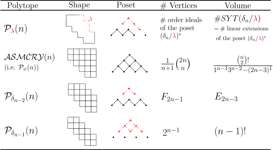
L_{\mathcal{P}_{\lambda}(n)}(t)=\Omega_{(\delta_{n}\backslash\lambda)^{*}}(t+1).

Note that using Theorem 3.4 and the discussion below it, we can express the volume and Ehrhart polynomial of any flow polytope as a Kostant partition function. Thus, Theorem 1.1 gives us several Kostant partition function identities. Corollaries 1.2, 5.10 and 5.11 compute the volumes and Ehrhart polynomials of three subfamilies of polytopes in ${\mathcal{F}}(ASM)(n)$ that are associated to posets with a nice number of linear extensions and vertices. This includes the ASM-CRY polytope. See Figure 9.

Proof of Corollary 1.2.

When $\lambda=\varnothing$ , ${\mathcal{P}}_{\varnothing}(n)$ is integrally equivalent to the order polytope $\mathcal{O}_{\delta_{n}^{*}}$ of the poset $\delta_{n}^{*}$ (that is, the type $A_{n-1}$ positive root lattice).

By Theorem 3.9 the number of vertices and volume of ${\mathcal{P}}_{\varnothing}(n)$ are given by the number of order ideals and linear extensions of the poset $\delta_{n}^{*}$ respectively. Next we compute each of these.

The order ideal of the poset $\delta_{n}^{*}$ correspond to shapes $\lambda\subseteq\delta_{n}$ which in turn correspond to Dyck paths counted by the Catalan number $C_{n}=\frac{1}{n+1}\binom{2n}{n}$ .

The number of linear extension of this poset is the number of standard Young tableaux (SYT) of shape $\delta_{n}=(n-1,n-2,\ldots,2,1)$ . Thus

{\rm vol}{\mathcal{P}}_{\varnothing}(n)=\#SYT(\delta_{n})=\frac{\binom{n}{2}!}{1^{n-1}3^{n-2}\cdots(2n-3)^{1}},

where the second equality follows by using the hook-length formula [27, Cor. 7.21.6] to compute this number of tableaux.

Lastly, by Theorem 3.9 $L_{{\mathcal{P}}_{\varnothing}(n)}(t)=\Omega_{\delta^{*}_{n}}(t+1)$ . When $t$ is an integer, $\Omega_{\delta^{*}_{n}}(t+1)$ counts the the number of plane partitions of shape $\delta_{n}$ with largest part $\leq t$ . By a result of Proctor [22] (see also [12]) this number is given by the product formula in the RHS of (1.1). ∎

Since the polytope ${\mathcal{CRY}}(n)$ is contained in ${\mathcal{ASMCRY}(n)}$ then we can bound the volume and number of lattice points of the former with the corresponding volume and number of lattice points of the latter.

Corollary 5.8.

For $n\geq 1$ and $t\in\mathbb{N}$ we have that

	$\displaystyle\prod_{i=1}^{n-2}{\rm Cat}(i)$	$\displaystyle\,\leq\,\#SYT(\delta_{n})$
	$\displaystyle L_{{\mathcal{CRY}}(n)}(t)$	$\displaystyle\,\leq\,\prod_{1\leq i<j\leq n}\frac{2t+i+j-1}{i+j-1}.$

Proof.

Since ${\mathcal{CRY}}(n)\subseteq{\mathcal{ASMCRY}(n)}$ and both polytopes have the same dimension then we can compare their normalized volumes to obtain ${\rm vol}({\mathcal{CRY}}(n))\leq{\rm vol}({\mathcal{ASMCRY}(n)})$ . Also by comparing the number of lattice points of their dilations we have that for $t$ in $\mathbb{N}$ , $L_{{\mathcal{CRY}}(n)}(t)\leq L_{{\mathcal{ASMCRY}(n)}}(t)$ . The result then follows by combining these bounds with Theorem 2.3 and Corollary 1.2 respectively. ∎

Remark 5.9.

Since the normalized volume of ${\mathcal{CRY}}(n)$ has a product formula, one wonders if there is a product formula for the number of its integer points; however, data suggests the answer to be negative (see data in [10, Sec. 6], [18] and [19]). It would interesting to study the asymptotics of $L_{{\mathcal{CRY}}(n)}(t)$ .

We give a few other examples of polytopes in the family ${\mathcal{F}}(ASM)(n)$ that have known nice formulas for the volume, namely, in the cases $\lambda=\delta_{n-k}$ for $k\geq 1$ . See Figure 9.

Let $[n]$ be the poset with $n$ elements and no relations and $z_{2n-1}$ and $z_{2n}$ denote the zigzag posets with $2n-1$ and $2n$ elements, respectively: and .

Corollary 5.10.

${\mathcal{P}}_{\delta_{n-1}}(n)$ is integrally equivalent to the order polytope ${\mathcal{O}}({[n-1]})$ of the antichain $[n-1]$ , it has $2^{n-1}$ vertices and its normalized volume equals $(n-1)!$ .

Proof.

Since the poset $[n-1]$ is an antichain, there are no relations, so the number of order ideals is $2^{n-1}$ and the number of linear extensions is $(n-1)!$ . Thus, the result follows from Theorem 1.1. ∎

Corollary 5.11.

${\mathcal{P}}_{\delta_{n-2}}(n)$ is integrally equivalent to the order polytope ${\mathcal{O}}({z_{2n-3}})$ of the zigzag poset $z_{2n-3}$ , its number of vertices is given by the Fibonacci number $F_{2n-1}$ , and its normalized volume is given by the Euler number $E_{2n-3}$ .

Proof.

The number of order ideals of the zigzag poset with $n$ elements is given by the Fibonacci number $F_{n+2}$ . To see this, note the posets $z_{0}$ and $z_{1}$ have $F_{2}=1$ and $F_{3}=2$ order ideals respectively. For the zigzag $z_{n}$ , the number of order ideals equals the sum of order ideals of $z_{n-1}$ and $z_{n-2}$ depending on whether or not the order ideals includes the leftmost (minimal) element of the poset. The result follows by induction.

The number of linear extensions of this poset is the number of SYT of skew shape ${\delta_{n}/\delta_{n-2}}$ which is given by the Euler number $E_{2n-3}$ . Thus, the result follows from Theorem 1.1. ∎

Remark 5.12.

For the case $\lambda=\delta_{n-k}$ , the polytope $\mathcal{P}_{\delta_{n-k}}(n)$ is integrally equivalent to the order polytope of the poset $(\delta_{n}\setminus\delta_{n-k})^{*}$ . The number of vertices of the polytope (order ideals of the poset) is given by the number of Dyck paths with height at most $k$ [24, A211216], [14, §3.1]. The volume of the polytope is given by the number of skew SYT of shape $\delta_{n}/\delta_{n-k}$ . There are formulas for this number of SYT as determinants of Euler numbers (e.g see Baryshnikov-Romik [4]).

We now turn from our investigation of the family of polytopes ${\mathcal{F}}(ASM)(n)$ to triangulations of flow and order polytopes.

6. Triangulations of flow polytopes of planar graphs

As we have seen in Section 3, flow polytopes of planar graphs are integrally equivalent to order polytopes. In this section we relate a known triangulation of flow polytopes by Danilov–Karzanov–Koshevoy and a well known triangulation of order polytopes.

6.1. Canonical triangulation of order polytopes

Recall that vertices of an order polytope ${\mathcal{O}}(P)$ correspond to characteristic functions of order filters (i.e. complements of order ideals). Stanley [26] gave a canonical way of triangulating the order polytope ${\mathcal{O}}(P)$ for an arbitrary poset $P$ . Namely, for a linear extension $(a_{1},a_{2},\ldots,a_{m})$ of the poset $P$ on elements $\{a_{1},a_{2},\ldots,a_{m}\}$ , define the simplex

(6.1)

\Delta_{a_{1},a_{2},\ldots,a_{m}}:=\{(x_{1},\ldots,x_{m})\in[0,1]^{m}\mid x_{a_{1}}\leq x_{a_{2}}\leq\cdots\leq x_{a_{m}}\}.

Note that the $m+1$ vertices of this simplex are $0,1$ vectors whose $0$ -coordinates are indexed by length $k$ prefixes $a_{1},\ldots,a_{k}$ of the linear extension for $k=0,1,\ldots,m$ . The simplices $\Delta_{a_{1},a_{2},\ldots,a_{m}}$ corresponding to all linear extensions of $P$ are top dimensional simplices in a triangulation of ${\mathcal{O}}(P)$ , which we refer to as the canonical triangulation of ${\mathcal{O}}(P)$ . There are also two established combinatorial ways of triangulating flow polytopes: one given by Postnikov and Stanley (PS) [21, 25] (defined in Section 7.1), and one by Danilov, Karzanov and Koshevoy (DKK) [9] (defined in Section 6.3). All the aforementioned triangulations are unimodular. The goal of this section is to relate the DKK triangulation of flow polytopes of planar graphs and Stanley’s linear extension triangulation of the corresponding order polytope.

As before, it will be more convenient for us to work with the integrally equivalent polytope $\widehat{{\mathcal{O}}}(P)\overset{\mathrm{int}}{\equiv}{\mathcal{O}}(P)$ and the integral equivalence $\nu$ from Lemma 3.8. The canonical triangulation of ${\mathcal{O}}(P)$ maps under $\nu^{-1}$ to the canonical triangulation of $\widehat{{\mathcal{O}}}(P)$ . We will denote $\nu^{-1}(\Delta_{a_{1},a_{2},\ldots,a_{m}})$ by $\widehat{\Delta}_{a_{1},a_{2},\ldots,a_{m}}$ . Of course:

(6.2)

\widehat{\Delta}_{a_{1},a_{2},\ldots,a_{m}}:=\{(x_{\hat{0}},x_{1},\ldots,x_{n},x_{\hat{1}})\in[0,1]^{m+2}\mid 0=x_{\hat{0}}\leq x_{a_{1}}\leq x_{a_{2}}\leq\cdots\leq x_{a_{m}}\leq x_{\hat{1}}=1\}.

In this section, we show that given a planar graph $G$ , the canonical triangulation of $\widehat{{\mathcal{O}}}(P_{G})$ maps to a DKK triangulation of ${\mathcal{F}}_{G}$ via the integral equivalence $\phi$ from Theorem 3.14. This result was first observed by Postnikov [21]. We also construct a direct bijection between linear extensions of $P_{G}$ , which index the canonical triangulation of $\widehat{{\mathcal{O}}}(P_{G})$ , and maximal cliques of $G$ , which index the DKK triangulation of ${\mathcal{F}}_{G}$ . In Section 7, we prove for a general graph $G$ that the DKK triangulations of ${\mathcal{F}}_{G}$ are framed Postnikov-Stanley triangulations of ${\mathcal{F}}_{G}$ . In particular, the canonical triangulation of $\widehat{{\mathcal{O}}}(P_{G})$ for a planar graph $G$ maps to a framed Postnikov-Stanley triangulation of ${\mathcal{F}}_{G}$ under integral equivalence $\phi$ from Theorem 3.14.

In the following subsection we review the results of Danilov, Karzanov and Koshevoy [9].

6.2. Danilov–Karzanov–Koshevoy triangulation of flow polytopes

Let $G$ be a connected graph on the vertex set $[n]$ with edges oriented from smaller to bigger vertices. Recall from Proposition 3.3, that vertices of ${\mathcal{F}}_{G}$ are given by unit flows along maximal directed paths from the source $1$ to the sink $n$ . Following [9], we call such maximal paths routes.

The following definitions also follow [9]. Let $v$ be an inner vertex of $G$ whenever $v$ is neither a source nor a sink. Fix a framing at each inner vertex $v$ , that is, a linear ordering $\prec_{{\it in}(v)}$ on the set of incoming edges ${\it in}(v)$ to $v$ and the linear ordering $\prec_{{\it out}(v)}$ on the set of outgoing edges ${\it out}(v)$ from $v$ . A framed graph, denoted by $(G,\prec)$ , is a graph $G$ with a framing $\prec$ at each inner vertex. For a framed graph $G$ and an inner vertex $v$ , we denote by ${\it In}(v)$ and by ${\it Out}(v)$ the set of maximal paths ending in $v$ and the set of maximal paths starting at $v$ , respectively. We define the order $\prec_{{\it In}(v)}$ on the paths in ${\it In}(v)$ as follows. If $P,Q\in{\it In}(v)$ , $P\neq Q$ , then let $w$ be the unique vertex after which $P$ and $Q$ coincide and before which they differ. Let $e_{P}$ be the edge of $P$ entering $w$ and $e_{Q}$ be the edge of $Q$ entering $w$ . Then $P\prec_{{\it In}(v)}Q$ if and only if $e_{P}\prec_{{\it in}(w)}e_{Q}$ . Similarly, if $P,Q\in{\it Out}(v)$ , $P\neq Q$ , then let $w$ be the unique vertex before which $P$ and $Q$ coincide and after which they differ. Let $e_{P}$ be the edge of $P$ leaving $w$ and $e_{Q}$ be the edge of $Q$ leaving $w$ . Then $P\prec_{{\it Out}(v)}Q$ if and only if $e_{P}\prec_{{\it out}(w)}e_{Q}$ .

Given a route $P$ with an inner vertex $v$ , denote by $Pv$ the maximal subpath of $P$ ending at $v$ and by $vP$ the maximal subpath of $P$ starting at $v$ . We say that the routes $P$ and $Q$ are coherent at a vertex $v$ which is an inner vertex of both $P$ and $Q$ if the paths $Pv,Qv$ are ordered the same way as $vP,vQ$ ; that is, $Pv\prec_{{\it In}(v)}Qv$ if and only if $vP\prec_{{\it Out}(v)}vQ$ . We say that routes $P$ and $Q$ are coherent if they are coherent at each common inner vertex. We call a set $C$ of mutually coherent routes a clique. Let $\mathcal{C}^{\max}(G,\prec)$ be the set of maximal cliques (with respect to number of routes) of the framed graph $G$ .

Definition 6.1.

Given a framed graph $G$ , and a clique $C$ of the framed graph $G$ , denote by $\Delta_{C}$ the convex hull of the vertices of ${\mathcal{F}}_{G}$ corresponding to the unit flows along routes in the clique $C$ .

Theorem 6.2 below is a special case of [9, Theorems 1 & 2].

Theorem 6.2.

[9, Theorems 1 & 2] Given a framed graph $(G,\prec)$ , the set of simplices

\{\Delta_{C}\mid C\in\mathcal{C}^{\max}(G,\prec)\},

corresponding to maximal cliques of the framed graph $G$ are the top dimensional simplices in a regular unimodular triangulation of ${\mathcal{F}}_{G}$ . Moreover, lower dimensional simplices $\Delta_{C}$ of this triangulation are obtained as convex hulls of the vertices corresponding to the routes in non-maximal cliques $\mathcal{C}$ of $G$ .

We call the triangulations specified in Theorem 6.2 the Danilov-Karzanov-Koshevoy (DKK) triangulations of ${\mathcal{F}}_{G}$ . Each such triangulation comes from a particular framing of the graph. We are now ready to prove that the canonical triangulation of $\widehat{{\mathcal{O}}}(P_{G})$ is integrally equivalent to a DKK triangulation of ${\mathcal{F}}_{G}$ via the map $\phi:\widehat{{\mathcal{O}}}(P_{G})\rightarrow{\mathcal{F}}_{G}$ from Theorem 3.14. We now define the framing needed for this result. Consider a planar graph $G$ on the vertex set $[n]$ with a particular planar embedding so that if vertex $i$ is in position $(x_{i},y_{i})$ then $x_{i}<x_{j}$ whenever $i<j$ . At each vertex $v\in[2,n-1]$ of $G$ there is a natural order on the edges coming from the planar drawing of the graph: order the incoming edges as well as the outgoing edges top to bottom in increasing order; by top to bottom we mean that if we put a small enough circle $C$ centered at vertex $i$ so that all incoming and outgoing edges to vertex $i$ intersect the circle, then we order the incoming (and outgoing) edges top to bottom by decreasing $y$ coordinates of their intersection with the circle $C$ . We call this framing the planar framing of $G$ , to emphasize that this framing comes from a particular planar embedding of the graph $G$ .

6.3. The canonical triangulation of $\widehat{{\mathcal{O}}}(P_{G})$ is integrally equivalent to a DKK triangulation of ${\mathcal{F}}_{G}$

We are now ready to state the main result of this section.

Theorem 1.3.

Given a planar graph $G$ , the canonical triangulation of $\widehat{{\mathcal{O}}}(P_{G})$ maps to the Danilov-Karzanov-Koshevoy triangulation of ${\mathcal{F}}_{G}$ coming from the planar framing via the integral equivalence map $\phi:\widehat{{\mathcal{O}}}(P_{G})\rightarrow{\mathcal{F}}_{G}$ given in Theorem 3.14.

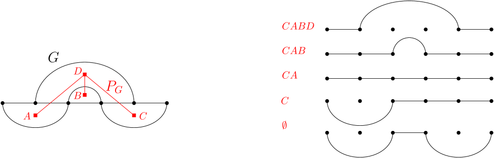
We prove Theorem 1.3 together with Theorem 6.6 below.

Recall that by Theorem 3.9 vertices of ${{\mathcal{O}}}(P_{G})$ are in bijection with order ideals of $P_{G}$ – indeed the vertices of ${{\mathcal{O}}}(P_{G})$ are the characteristic functions of the complements of the order ideals in the poset $P_{G}$ . By Lemma 3.8 the vertices of $\widehat{{\mathcal{O}}}(P_{G})$ are also naturally indexed by the order ideals of $P_{G}$ . Let $f_{I}$ be the vertex of $\widehat{{\mathcal{O}}}(P_{G})$ indexed by the order ideal $I$ of $P_{G}$ . Given a planar graph $G$ we say that a route $R$ of $G$ separates the order ideal $I$ and the complement $P_{G}\setminus I$ if the elements of $P_{G}$ below the route $R$ in the planar drawing of $G$ and the truncated dual $P_{G}$ are exactly the elements of the order ideal $I$ .

Proposition 6.3.

Given a vertex $f_{I}$ of $\widehat{{\mathcal{O}}}(P_{G})$ indexed by the order ideal $I$ of $P_{G}$ we have that $\phi(f_{I})$ is the unit flow along the route $R$ in $G$ separating $I$ and $P_{G}\setminus I$ . Moreover, any route $R$ in $G$ separates some order ideal $I$ and $P_{G}\setminus I$ .

Proof.

As explained in Section 3, the elements of $P_{G}$ correspond to bounded regions defined by $G$ . Given an indicator function $f_{I}$ for the complement of an order ideal $I$ of this poset, by Definition 3.15 the flow $\phi(f_{I})$ is the specified unit flow. See Figure 11 for an example. ∎

Next, we define the map $\Phi_{\Delta}$ between linear extensions of $P_{G}$ , which index the top dimensional simplices in the canonical triangulations of $\widehat{O}(P_{G})$ , and sets of routes corresponding to the vertices of top dimensional simplices in a DKK triangulation of ${\mathcal{F}}_{G}$ (the latter is shown in Theorem 6.6).

Definition 6.4.

Given a linear extension ${\bf a}=a_{1}\cdots a_{m}$ of $P_{G}$ , let $\Phi_{\Delta}({\bf a})$ be the following set of routes of $G$ determined by the order ideals whose elements are the letters in the prefixes of ${\bf a}$ ,

\Phi_{\Delta}({\bf a})\,:=\,\{\phi(f_{\{a_{1},\cdots,a_{k}\}})\mid k=0,1,\ldots,m\}.

That is, $\Phi_{\Delta}({\bf a})$ is the set of routes of $G$ separating each of the order ideals formed from letters in the prefixes of the linear extension $a_{1},\ldots,a_{m}$ . See Figure 11 for an example.

Next, we show that the routes in $\Phi_{\Delta}({\bf a})$ form a clique.

Lemma 6.5.

For a planar graph $G$ , fix a linear extension ${\bf a}=a_{1}\cdots a_{m}$ of $P_{G}$ indexing a simplex $\widehat{\Delta}_{a_{1}\cdots a_{m}}$ of $\widehat{O}(P_{G})$ . Then the routes in $\Phi_{\Delta}({\bf a})$ are pairwise coherent in the planar framing of $G$ .

Proof.

Let $v_{1}$ and $v_{2}$ be vertices of $\widehat{\Delta}_{a_{1}\cdots a_{m}}$ mapping to routes $P_{1}$ and $P_{2}$ under $\phi_{v}$ . It suffices to show that $P_{1}$ and $P_{2}$ are coherent in the planar framing of $G$ .

Let the coordinates of $v_{1}$ equal to $0$ be $x_{\hat{0}},x_{a_{1}},\ldots,x_{a_{k_{1}}}$ and the coordinates of $v_{2}$ equal to $0$ be $x_{\hat{0}},x_{a_{1}},\ldots,x_{a_{k_{2}}}$ and assume without loss of generality that $k_{1}<k_{2}$ . Since both ${a_{1}},\ldots,{a_{k_{1}}}$ and ${a_{1}},\ldots,{a_{k_{2}}}$ are prefixes of the linear extension of ${a_{1}},\ldots,{a_{m}}$ , we see that the upper boundary of the regions corresponding to ${a_{1}},\ldots,{a_{k_{1}}}$ lies weakly below that of the boundary of the regions corresponding to ${a_{1}},\ldots,{a_{k_{2}}}$ , and thereby the corresponding routes $P_{1}$ and $P_{2}$ are coherent with respect to the planar framing. ∎

Theorem 6.6.

Given a planar graph $G$ , the map $\Phi_{\Delta}$ defined above is a bijection between linear extensions of $P_{G}$ and maximal cliques in $G$ in the planar framing.

Proof of Theorems 1.3 & 6.6..

By Theorem 3.14, $\phi$ is an integral equivalence between $\widehat{{\mathcal{O}}}(P_{G})$ and ${\mathcal{F}}_{G}$ . In particular, the polytopes $\widehat{{\mathcal{O}}}(P_{G})$ and ${\mathcal{F}}_{G}$ are of the same dimension and same relative volume. Therefore, the top dimensional simplices in their respective triangulations have the same number of vertices, and the number of simplices in any of their unimodular triangulations are the same. Thus, to show Theorems 1.3 & 6.6 it suffices to show that $\phi$ restricts to a bijection on the vertices of $\widehat{{\mathcal{O}}}(P_{G})$ and ${\mathcal{F}}_{G}$ and that the set of routes that $\Phi_{\Delta}$ maps a linear extension to are pairwise coherent in the planar framing. The former is follows from Proposition 6.3, while the latter from Lemma 6.5. ∎

Corollary 6.7.

Given a planar graph $G$ , the number of linear extensions of $P_{G}$ equals the number of maximal cliques in $G$ in any framing.

Proof.

The statement is immediate from Theorem 1.3 for the planar framing. But since the Danilov-Karzanov-Koshevoy triangulations are unimodular, the number of maximal cliques in $G$ is independent of the framing. ∎

7. Triangulations of flow polytopes of general graphs

In Theorem 6.6 we gave a bijection from linear extensions of $P_{G}$ to maximal cliques of $G$ in the planar framing. In this section we will see that given any two framings of a graph $G$ (not necessarily planar) there is a natural bijection between their sets of maximal cliques. Therefore, combining the bijection from Theorem 6.6 and the one just mentioned, we obtain a bijection between linear extensions of $P_{G}$ and maximal cliques in any framing of a planar graph $G$ .

More generally, this section is devoted to studying the set of DKK triangulations of a flow polytope ${\mathcal{F}}_{G}$ and the framed Postnikov-Stanley (PS) triangulations of ${\mathcal{F}}_{G}$ , which we define in this section. We show that the set of DKK triangulations of a flow polytope ${\mathcal{F}}_{G}$ is equal the set of framed PS triangulations of ${\mathcal{F}}_{G}$ . As a consequence of our proof, we obtain a bijection between the objects indexing the PS triangulation of a flow polytope ${\mathcal{F}}_{G}$ , namely, nonnegative integer flows on the graph $G$ with netflow $(0,d_{2},\ldots,d_{n-1},-\sum_{i=2}^{n-1}d_{i})$ , where $d_{i}$ is the indegree of vertex $i$ in $G$ minus $1$ ¹¹1See Definition 3.1 and the discussion in Section 3.1 for the relation of nonnegative integer flows with a given netflow vector to Kostant partition functions as well as Theorem 3.4., and the objects indexing the DKK triangulation of a flow polytope ${\mathcal{F}}_{G}$ , namely, maximal cliques in a fixed framing of $G$ . This answers Postnikov’s question [21] about a bijection between the sets indexing the maximal simplices of both triangulations. We also obtain a natural bijection between the sets of maximal cliques of $G$ in different framings, as mentioned in the previous paragraph.

7.1. Framed Postnikov-Stanley triangulations

We now define framed Postnikov-Stanley triangulations. These triangulations were used in [16], though they were not described explicitly there, and we follow closely the exposition therein.

A bipartite noncrossing tree is a tree with left vertices $x_{1},\ldots,x_{\ell}$ and right vertices $x_{\ell+1},\ldots,x_{\ell+r}$ with no pair of edges $(x_{p},x_{\ell+q}),(x_{t},x_{\ell+u})$ where $p<t$ and $q>u$ . We denote by $\mathcal{T}_{{\mathcal{I}},{\mathcal{O}}}$ the set of bipartite noncrossing trees where ${\mathcal{I}}$ and ${\mathcal{O}}$ are the ordered sets $(x_{1},\ldots,x_{\ell})$ and $(x_{\ell+1},\ldots,x_{\ell+r})$ respectively. We have that $\#\mathcal{T}_{{\mathcal{I}},{\mathcal{O}}}=\binom{\ell+r-2}{\ell-1}$ , since the elements of $\mathcal{T}_{{\mathcal{I}},{\mathcal{O}}}$ are in bijection with weak compositions of $\ell-1$ into $r$ parts. A tree $T$ in $\mathcal{T}_{{\mathcal{I}},{\mathcal{O}}}$ corresponds to the composition $(b_{1},\ldots,b_{r})$ of $(\text{indegrees $-1$})$ , where $b_{i}$ denotes the number of edges incident to the right vertex $x_{\ell+i}$ in $T$ minus $1$ .

Example 7.1.

The bipartite tree in Figure 13 corresponds to the composition $(1,0,2)$ .

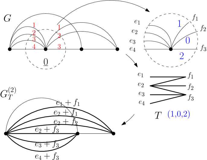
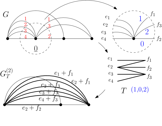
We now define what we mean by a reduction at vertex $i$ of a framed graph $G$ on the vertex set $[n]$ . Let ${\mathcal{I}}_{i}$ denote the multiset of incoming edges and ${\mathcal{O}}_{i}$ the multiset of outgoing edges of $i$ . In addition, we assume that ${\mathcal{I}}_{i}$ and ${\mathcal{O}}_{i}$ are linearly ordered according to the framing of $G$ . A reduction performed at $i$ of $G$ results in several new graphs indexed by bipartite noncrossing trees on the left vertex set $I_{i}$ and right vertex set ${\mathcal{O}}_{i}$ . We define these new graphs precisely below.

Consider a tree $T\in\mathcal{T}_{\mathcal{I}_{i},\mathcal{O}_{i}}$ . For each tree-edge $(e_{1},e_{2})$ of $T$ where $e_{1}=(r,i)\in\mathcal{I}_{i}$ and $e_{2}=(i,s)\in\mathcal{O}_{i}$ , let $e_{1}+e_{2}$ be the following edge:

(7.1)

e_{1}+e_{2}=(r,s).

We call the edge $e_{1}+e_{2}$ the sum of edges. Alternatively you can consider this as a path in $G$ consisting of edges $e_{1}$ and $e_{2}$ . Inductively, we can also define the sum of more than two consecutive edges.

Given $T$ in $\mathcal{T}_{\mathcal{I}_{i},\mathcal{O}_{i}}$ , let $G^{(i)}_{T}$ be the graph obtained from $G$ by removing the vertex $i$ and all the edges of $G$ incident to $i$ and adding the multiset of edges $\{\{e_{1}+e_{2}~|~(e_{1},e_{2})\in E(T)\}\}$ . See Figures 12, 15 and 14 for examples of $G^{(i)}_{T}$ .

Given a tree $T$ in $\mathcal{T}_{{\mathcal{I}}_{i},{\mathcal{O}}_{i}}$ , a reduction of $G$ at the vertex $i$ with respect to $T$ replaces $G$ by the graphs in $G^{(i)}_{T}$ defined above. The reduction also keeps track which sum of the edges of $G$ is each edge of the new graphs (allowing for the sum of only one element, when an edge was left intact).

We now define an inheritance framing of $G^{(i)}_{T}$ for $T$ in $\mathcal{T}_{{\mathcal{I}}_{i},{\mathcal{O}}_{i}}$ , which it inherits from the framing of $G$ as follows:

(i)

The edges incident to a vertex $j$ smaller than $i$ in $G^{(i)}$ are in bijection with edges incident to vertex $j$ in $G$ . We order the edges in $G^{(i)}$ in the same way as they are ordered in $G$ .
(ii)

For each vertex $j$ greater than $i$ the multiset of outgoing edges ${\mathcal{O}}_{j}(G^{(i)}_{T})$ equals ${\mathcal{O}}_{j}(G)$ . We order these the edges of ${\mathcal{O}}_{j}(G^{(i)}_{T})$ the same way the edges ${\mathcal{O}}_{j}(G)$ are ordered.
(iii)

For each vertex $j$ greater than $i$ , if ${\mathcal{I}}_{j}(G)=\{m_{1},\ldots,m_{k}\}$ (the multiset linearly ordered according to the framing of $G$ ), then the multiset ${\mathcal{I}}_{j}(G^{(i)}_{T})$ consists of edges that are sums of edges of $G$ (potentially the empty sum) with an edge of ${\mathcal{I}}_{j}(G)$ . Thus denote by $S(m_{l})$ , $l\in[k]$ , the edges in ${\mathcal{I}}_{j}(G^{(i)}_{T})$ which are sums of edges of $G$ (potentially the empty sum) with $m_{l}$ . Then let any edge in $S(m_{p})$ be less than any edge in $S(m_{q})$ for $p<q$ , $p,q\in[k]$ . We now specify the ordering of the edges within the sets $S(m_{l})$ , $l\in[k]$ . If $S(m_{l})=\{m_{l}\}$ then there is nothing to specify. If $S(m_{l})\neq\{m_{l}\}$ , then draw $T$ with the left and right sets of vertices ordered vertically following the linear order of ${\mathcal{I}}_{i}$ and ${\mathcal{O}}_{i}$ from the framing of $G$ . We order the edges in $S(m_{l})$ following the order on the edges of the noncrossing bipartite tree $T$ when viewed from top to bottom (smallest edge to largest). See Figure 13 for an example.

Next we describe what we refer to as the framed Postnikov-Stanley (PS) triangulations of ${\mathcal{F}}_{G}$ .

Given a framed graph $(G,\prec)$ on the vertex set $[n]$ , and a nonnegative integer flow ${\rm ifl}(\cdot)$ on $G$ with netflow $(0,d_{2},d_{3},\ldots,d_{n-1},-\sum_{i}d_{i})$ , where $d_{i}=indeg_{i}(G)-1$ , we explain how to obtain a simplex $\Delta_{{\rm ifl}}^{(G,\prec)}$ , such that as ${\rm ifl}$ runs over all nonnegative integer flow $G$ with netflow $(0,d_{2},d_{3},\ldots,d_{n-1},-\sum_{i}d_{i})$ we obtain a set of simplices $\Delta_{{\rm ifl}}^{(G,\prec)}$ that are the top dimensional simplices of a triangulation of ${\mathcal{F}}_{G}$ . It is this triangulation that we term the framed Postnikov-Stanley (PS) triangulation.

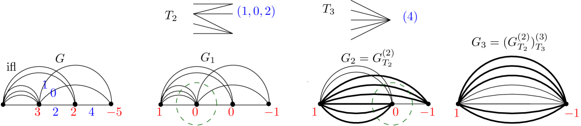
Given a framed graph $(G,\prec)$ on the vertex set $[n]$ , and a nonnegative integer flow ${\rm ifl}(\cdot)$ on $G$ with netflow $(0,d_{2},d_{3},\ldots,d_{n-1},-\sum_{i}d_{i})$ we read off the nonnegative integer flow values specified by ${\rm ifl}(\cdot)$ on the edges of $\mathcal{O}_{2}(G)$ yielding a composition $(c_{1},\ldots,c_{\#\mathcal{O}_{2}(G)})$ of $d_{2}=\#\mathcal{I}_{2}(G)-1$ . Here $c_{j}$ corresponds to the flow value on the $j$ th largest edge in $\mathcal{O}_{2}(G)$ in the framing. Using this composition $(c_{1},\ldots,c_{\#\mathcal{O}_{2}(G)})$ of $d_{2}=\#\mathcal{I}_{2}(G)-1$ , we build a bipartite tree $T_{2}$ in $\mathcal{T}_{{\mathcal{I}}_{2},{\mathcal{O}}_{2}}$ as follows. The sets ${\mathcal{I}}_{2}$ and ${\mathcal{O}}_{2}$ have an ordering in the framing of $G$ . Assume that this ordering is ${\mathcal{I}}_{2}=\{v_{1}<\cdots<v_{\#{\mathcal{I}}_{2}}\}$ and ${\mathcal{O}}_{2}=\{w_{1}<\cdots<w_{\#{\mathcal{O}}_{2}}\}$ . Draw the bipartite tree $T_{2}$ in $\mathcal{T}_{{\mathcal{I}}_{2},{\mathcal{O}}_{2}}$ with the left vertex set ${\mathcal{I}}_{2}=\{v_{1}<\cdots<v_{\#{\mathcal{I}}_{2}}\}$ so that the vertices $v_{1}<\cdots<v_{\#{\mathcal{I}}_{2}}$ are ordered top to bottom vertically on the left. Similarly, the right vertices $w_{1}<\cdots<w_{\#{\mathcal{O}}_{2}}$ are drawn top to bottom vertically on the right. We let the degree of vertex $w_{j}$ in $T_{2}$ be $c_{j}+1$ . The above uniquely determines the noncrossing bipartite tree $T_{2}$ on left and right vertex sets ${\mathcal{I}}_{2}$ and ${\mathcal{O}}_{2}$ . See Figure 12 for an example. With tree $T_{2}$ constructed, we do a reduction at vertex $2$ to obtain $G_{2}:=G_{T_{2}}^{(2)}$ with an inheritance framing.

Recursively, given $G_{i-1}$ , we read off the integer flow values from ${\rm ifl}(\cdot)$ on the edges of $\mathcal{O}_{i}(G)=\mathcal{O}_{i}(G_{i-1})$ . These flow values can be seen as components of a composition $(c_{1},\ldots,c_{\#\mathcal{O}_{i}(G)})$ of

d_{i}+\sum_{e,{\rm fin}(e)=i}{\rm ifl}(e)\,=\,\#\mathcal{I}_{i}(G_{i-1})-1.

The component $c_{j}$ corresponds to the flow value on the $j$ th largest edge in $\mathcal{O}_{i}(G)=\mathcal{O}_{i}(G_{i-1})$ in the framing. From this composition $(c_{1},\ldots,c_{\#\mathcal{O}_{i}(G)})$ we build a bipartite tree $T_{i}$ in $\mathcal{T}_{\mathcal{I}_{i}(G_{i-1}),\mathcal{O}_{i}(G_{i-1})}$ as follows. The sets $\mathcal{I}_{i}(G_{i-1})$ and $\mathcal{O}_{i}(G_{i-1})$ have an ordering in the inheritance framing of $G_{i-1}$ . Assume that this ordering is $\mathcal{I}_{i}(G_{i-1})=\{v_{1}<\cdots<v_{\#\mathcal{I}_{i}(G_{i-1})}\}$ and $\mathcal{O}_{i}(G_{i-1})=\{w_{1}<\cdots<w_{\#\mathcal{O}_{i}(G_{i-1})}\}$ . Draw the bipartite tree $T_{i}$ in $\mathcal{T}_{\mathcal{I}_{i}(G_{i-1}),\mathcal{O}_{i}(G_{i-1})}$ with the left vertex set $\mathcal{I}_{i}(G_{i-1})=\{v_{1}<\cdots<v_{\#\mathcal{I}_{i}(G_{i-1})}\}$ so that the vertices $v_{1}<\cdots<v_{\#\mathcal{I}_{i}(G_{i-1})}$ are ordered top to bottom vertically on the left. Similarly, the right vertices $w_{1}<\cdots<w_{\#\mathcal{O}_{i}(G_{i-1})}$ are drawn top to bottom vertically on the right. We let the degree of vertex $w_{j}$ in $T_{i}$ be $c_{j}+1$ . The above uniquely determines the noncrossing bipartite tree $T_{i}$ on left and right vertex sets $\mathcal{I}_{i}(G_{i-1})$ and $\mathcal{O}_{i}(G_{i-1})$ . With tree $T_{i}$ constructed we do a reduction at vertex $i$ to obtain $G_{i}:=(G_{i-1})_{T_{i}}^{(i)}$ with an inheritance framing. We iterate this for $i=1,\ldots,n-1$ . See Figure 14 for an example.

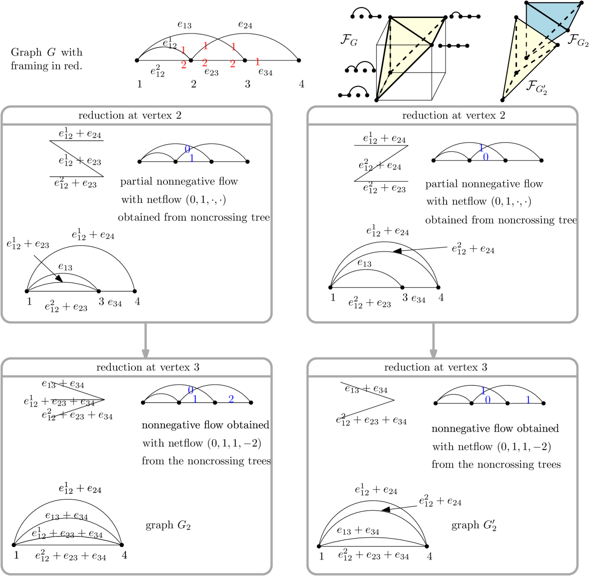
Thus, from the integer flow ${\rm ifl}(\cdot)$ we obtain a tuple of bipartite noncrossing trees $(T_{2},T_{3},\ldots,T_{n-1})$ such that $G_{i}:=(G_{i-1})_{T_{i}}^{(i)}$ for $i=2,\ldots,n-1$ and $G_{1}:=G$ . Since $G_{n-1}$ has no incoming or outgoing edges to vertices $i=2,\ldots,n-1$ then $G_{n-1}$ consists of two vertices $1$ and $n$ and $\#E(G)-n+2$ multiple edges. Thus $\mathcal{F}_{G_{n-1}}$ is a $(\#(G)-n+1)$ -simplex.

Recall that each such multiple edge $e$ in $\mathcal{F}_{G_{n-1}}$ is a sum of edges of the original graph of $G$ as explained in the beginning of this section. Such sum of edges corresponds to a route in the graph $G$ , i.e. a directed path from vertex $1$ and $n$ in $G$ . We denote the unit flow in $G$ along the route corresponding to edge $e$ in $G_{n-1}$ by $\rho(e)$ and we let

\Delta_{{\rm ifl}}^{(G,\prec)}:={\rm ConvHull}\{\rho(e)\mid e\in E({G_{n-1}})\}

be the simplex with vertices $\rho(e)$ . Note that $\Delta_{{\rm ifl}}^{(G,\prec)}$ is integrally equivalent to $\mathcal{F}_{G_{n-1}}$ , and it is a subset of $\mathcal{F}_{G}$ .

Postnikov and Stanley proved Theorem 3.4 by showing that this iterative construction of simplices from integer flows yields a triangulation of $\mathcal{F}_{G}$ . Denote by ${\mathcal{F}}_{G}^{{\rm int}}(0,d_{2},\ldots,d_{n-1},-\sum_{i}d_{i})$ the set of nonnegative integer flows on the graph $G$ with netflow $(0,d_{2},\ldots,d_{n-1},-\sum_{i}d_{i})$ .

Theorem 7.2 (cf. [16, §6.1]).

Given a framed graph $(G,\prec)$ , the set of simplices

\{\Delta_{{\rm ifl}}^{(G,\prec)}\mid{\rm ifl}\in{\mathcal{F}}_{G}^{{\rm int}}(0,d_{2},\ldots,d_{n-1},-\sum_{i}d_{i})\},

where $d_{i}=indeg_{i}(G)-1$ , are the top simplices of a unimodular triangulation of ${\mathcal{F}}_{G}$ .

Remark 7.3.

Note that the triangulation in [16, §6.1] comes from the top to bottom framing of the graph. Theorem 7.2 yields a triangulation for any framing of the graph. The proof in [16, §6.1] adapts readily for an arbitrary framing. Indeed, more general triangulations can be constructed in the above way that do not depend on a fixed framing of the graph $G$ ; we only need to specify some (any) ordering of edges at each vertex as we do the reductions.

7.2. The set of DKK triangulations equals the set of framed PS triangulations

In this section we show that with a fixed framing $(G,\prec)$ the DKK triangulations and the PS triangulation are identical. In effect, the set of DKK triangulations equals the set of framed PS triangulations. We also give an explicit bijection between the objects indexing a DKK triangulation of ${\mathcal{F}}_{G}$ for a framing of $G$ and a framed PS triangulation of ${\mathcal{F}}_{G}$ , namely a bijection between maximal cliques of $G$ with respect to a fixed framing and nonnegative integer flows of $G$ with netflow $(0,d_{2},\ldots,d_{n-1},-\sum_{i}d_{i})$ .

The following results show that the vertices of a simplex $\Delta_{{\rm ifl}}^{(G,\prec)}$ correspond to a maximal clique of the framed graph $(G,\prec)$ . Recall that the simplex $\Delta_{{\rm ifl}}^{(G,\prec)}$ is integrally equivalent to the flow polytope ${\mathcal{F}}_{G_{n-1}}$ of a graph $G_{n-1}$ consisting of vertices $1$ and $n$ and $\#E(G)-n+2$ multiple edges $(1,n)$ and that the set of simplices $\Delta_{{\rm ifl}}^{(G,\prec)}$ , as ${\rm ifl}$ runs over all flows in ${\mathcal{F}}_{G}^{{\rm int}}(0,d_{2},d_{3},d_{4},d_{5},-\sum_{i}d_{i})$ forms the top dimensional simplices of a unimodular triangulation of ${\mathcal{F}}_{G}$ as shown in Theorem 7.2.

Proposition 7.4.

Given a framed graph $(G,\prec)$ with vertices $[n]$ and a nonnegative integer flow ${\rm ifl}\in{\mathcal{F}}_{G}^{{\rm int}}(0,d_{2},d_{3},d_{4},d_{5},-\sum_{i}d_{i})$ , where $d_{i}=indeg_{i}(G)-1$ , the routes of $G$ along which the unit flows give the vertices of the simplex $\Delta_{{\rm ifl}}^{(G,\prec)}$ form a maximal clique with respect to the coherence relation in $(G,\prec)$ .

Proof.

Recall that $\Delta_{{\rm ifl}}^{(G,\prec)}\overset{\mathrm{int}}{\equiv}{\mathcal{F}}_{G_{n-1}}$ , for some $G_{n-1}$ as described in Section 7.1. Recall that a sequence of graphs $G_{1}:=G,G_{2},\ldots,G_{n-1}$ encode the successive reductions leading to the simplex $\Delta_{{\rm ifl}}^{(G,\prec)}\overset{\mathrm{int}}{\equiv}{\mathcal{F}}_{G_{n-1}}$ . Graph $G$ has a framing, and the framing of graph $G_{i}$ , $i\in[2,n-1]$ , is the inheritance framing obtained from the framing of $G_{i-1}$ . Suppose that to the contrary, there are two vertices of the simplex $\Delta_{{\rm ifl}}^{(G,\prec)}$ , which correspond to non-coherent routes $P$ and $Q$ in $G$ . Suppose that $P$ and $Q$ are not coherent at the common inner vertex $v$ . Suppose that the smallest vertex after which $Pv$ and $Qv$ agree is $w_{1}$ and the largest vertex before which $vP$ and $vQ$ agree is $w_{2}$ . Let the edges incoming to $w_{1}$ be $e_{P}^{1}$ and $e_{Q}^{1}$ for $P$ and $Q$ , respectively, and let the edges outgoing from $w_{2}$ be $e_{P}^{2}$ and $e_{Q}^{2}$ for $P$ and $Q$ , respectively. Since $P$ and $Q$ are not coherent at $v$ , this implies that either $e_{P}^{1}\prec_{{\it in}(w_{1})}e_{Q}^{1}$ and $e_{Q}^{2}\prec_{{\it out}(w_{2})}e_{P}^{2}$ or $e_{Q}^{1}\prec_{{\it in}(w_{1})}e_{P}^{1}$ and $e_{P}^{2}\prec_{{\it out}(w_{2})}e_{Q}^{2}$ . We also have that the segments of $P$ and $Q$ between $w_{1}$ and $w_{2}$ coincide.

Denote by $p$ the sum of edges between $w_{1}$ and $w_{2}$ on $P$ . Denote by $*(e_{{Z}}^{1}+p)$ , for $Z\in\{P,Q\}$ , the sum of edges left of $w_{2}$ that are edges in ${Z}$ (including $e_{{Z}}^{1}$ in particular). After a certain number of reductions executed according to the framing, we are about to perform the reduction at vertex $w_{2}$ . This reduction involves deleting $w_{2}$ and the edges incident to it, and adding the edges obtained from the noncrossing tree $T$ we constructed based on the ordering of the incoming and outgoing edges at $w_{2}$ . In such a noncrossing tree, the vertex corresponding to the edge stemming from $*(e_{{Z}}^{1}+p)$ , $Z\in\{P,Q\}$ , is above the vertex $*(e_{{\overline{Z}}}^{1}+p)$ , where $\overline{Z}$ is the complement of $Z$ in $\{P,Q\}$ , in the left partition of the vertices of $T$ . On the other hand, the vertex corresponding to $e_{\overline{Z}}^{2}$ is above the vertex corresponding to $e_{Z}^{2}$ in the right partition of the vertices of $T$ . Thus, it is impossible to obtain both routes $P$ and $Q$ as vertices of ${\mathcal{F}}_{G_{n-1}}$ since that would force connecting $*(e_{{Z}}^{1}+p)$ and $e_{{Z}}^{2}$ as well as $*(e_{\overline{Z}}^{1}+p)$ and $e_{\overline{Z}}^{2}$ in $T$ . This would make a crossing in the noncrossing tree $T$ , a contradiction. ∎

Proposition 7.4 justifies the following definition.

Definition 7.5.

Given a framed graph $(G,\prec)$ on the vertex set $[n]$ , let

\Lambda^{(G,\prec)}:\mathcal{F}^{{\rm int}}_{G}(0,d_{2},\ldots,d_{n-1},\sum_{i}d_{i})\to\mathcal{C}^{\max}(G,\prec)

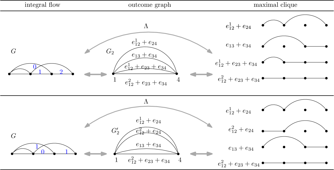
be the map defined by $\Lambda^{(G,\prec)}({\rm ifl})=C$ , where the vertices of the simplex $\Delta_{{\rm ifl}}^{(G,\prec)}$ are the unit flows along routes in the maximal clique $C$ and $d_{i}=indeg_{i}(G)-1$ .

Example 7.6.

Figure 17 gives an example of the bijection $\Lambda^{(G,\prec)}$ between the two integer flows in ${\mathcal{F}}^{{\rm int}}_{G}(0,d_{2},d_{3},-d_{2}-d_{3})$ and the two maximal cliques with respect to the framing of $G$ given in Figure 14.

Example 7.7.

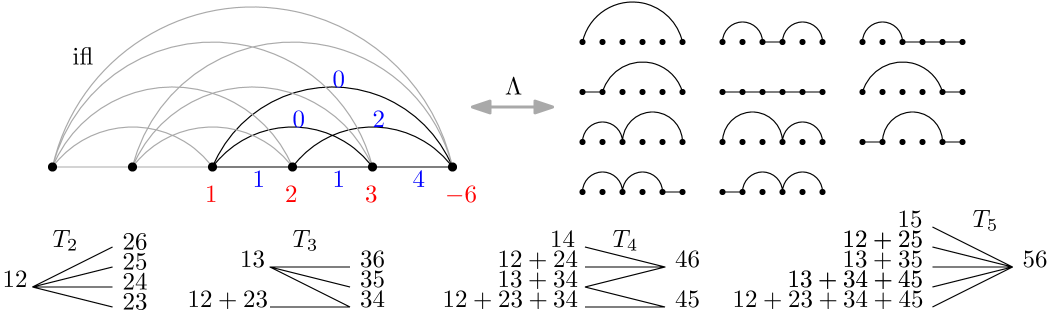
Figure 16 gives a larger example of the bijection $\Lambda^{(G,\prec)}$ between an integer flow in ${\mathcal{F}}^{{\rm int}}_{K_{6}}(0,0,1,2,-3)$ and a maximal clique of $K_{6}$ .

We now have:

Theorem 7.8.

Given a framed graph $(G,\prec)$ on the vertex set $[n]$ the Danilov-Karzanov-Koshevoy triangulations of ${\mathcal{F}}_{G}$ with respect to this framing is the framed Postnikov-Stanley triangulations of ${\mathcal{F}}_{G}$ with respect to the same framing. Moreover, the map $\Lambda^{(G,\prec)}$ defined above is a bijection between nonnegative integer flows in $\mathcal{F}_{G}^{{\rm int}}(0,d_{2},\ldots,d_{n-1},-\sum_{i}d_{i})$ , where $d_{i}=indeg_{i}(G)-1$ , and maximal cliques in $\mathcal{C}^{\max}(G,\prec)$ .

Proof.

Fix a framing $(G,\prec)$ . Proposition 7.4 shows that the framed PS triangulation with respect to this framing is the same as the DKK triangulation with respect to this framing. Therefore, any DKK triangulation is a framed PS triangulation. In particular, $\Lambda^{(G,\prec)}$ is a bijection that simply sends one set of labelings of a fixed triangulation of ${\mathcal{F}}_{G}$ into another set of labelings of the very same triangulation of ${\mathcal{F}}_{G}$ . ∎

We conclude by noting that there is a nice way to describe the inverse of the map $\Lambda^{(G,\prec)}$ :

Lemma 7.9.

Fix a framed graph $(G,\prec)$ and a flow ${\rm ifl}\in{\mathcal{F}}_{G}^{{\rm int}}(0,d_{2},\ldots,d_{n-1},-\sum_{i}d_{i})$ , where $d_{i}=indeg_{i}(G)-1$ . If $\Lambda^{(G,\prec)}({\rm ifl})=C$ , then each edge $e$ of the graph $G$ appears ${\rm ifl}(e)+1$ times as an edge of one of the paths ending in $v={{\rm fin}(e)}$ in the set (not multiset!) $\{Pv\mid P\in C,v={{\rm fin}(e)}\}$ of prefixes of routes in the clique $C$ . In particular, given a maximal clique $C\in\mathcal{C}^{\max}(G,\prec)$ the inverse $(\Lambda^{(G,\prec)})^{-1}(C)$ is given by

((\Lambda^{(G,\prec)})^{-1}(C))(e)=n(e)-1,

where $n(e)$ is the number of times edge $e$ appears in set of prefixes $\{Pv\mid P\in C,v={{\rm fin}(e)}\}$ .

Proof.

By the construction of $\Lambda^{(G,\prec)}$ , from the integer flow ${\rm ifl}(\cdot)$ we obtain a tuple of noncrossing bipartite trees $(T_{2},T_{3},\ldots,T_{n-1})$ such that $G_{1}=G$ and $G_{i}:=(G_{i-1})^{(i)}_{T_{i}}$ for $i=2,\ldots,n-1$ where $G_{n-1}$ is a graph with vertices $1$ and $n$ and $\#E(G)-n+2$ multiple edges where each multiple edge is a sum of edges of the original graph $G$ defining a route of the maximal clique $C$ .

The edges of intermediate graphs $G_{2},\ldots,G_{n-2}$ for $i=2,\ldots,n-2$ encode prefixes of the routes in the clique $C$ as follows: for the edge $e=(i,j)$ in $\mathcal{O}_{i}(G)=\mathcal{O}_{i}(G_{i-1})$ , the tree $T_{i}$ in $\mathcal{T}_{\mathcal{I}_{i}(G_{i-1}),\mathcal{O}_{i}(G_{i-1})}$ has ${\rm ifl}(e)+1$ tree-edges incident to $e$ by definition. Therefore, the edge $e$ appears exactly ${\rm ifl}(e)+1$ times in the set of prefixes of the routes $\{Pv\mid P\in C,v={{\rm fin}(e)}\}$ . The statement about $(\Lambda^{(G,\prec)})^{-1}(C)$ then follows readily. ∎

Example 7.10.

We continue with Example 7.7 illustrated in Figure 16. Edge $e=(3,4)$ has flow ${\rm ifl}(e)=1$ and there are two paths ending in vertex $4$ containing $e$ in the corresponding clique $C:=\Lambda^{(G,\prec)}({\rm ifl})$ , namely the paths consisting of edges $(1,2),(2,3),(3,4)$ and of edges $(1,3),(3,4)$ . Note that the path $(1,3),(3,4)$ is the prefix of two routes in the clique, however, we count it here just once since in Lemma 7.9 we are looking at the set of prefixes of the routes in the clique and not a multiset of prefixes.

Acknowledgments

The authors are grateful to Alexander Postnikov for generously sharing his insights and questions. The authors are also grateful to the anonymus referee for numerous helpful comments and suggestions. AHM and JS would like to thank ICERM and the organizers of its Spring 2013 program in Automorphic Forms during which part of this work was done. The authors also thank the SageMath community [28] for developing and sharing their code by which some of this research was conducted.

References

[1] W. Baldoni-Silva and M. Vergne. Kostant partition functions and flow polytopes. Transform. Groups, 13(3-4):447–469, 2008.
[2] Y. Baryshnikov and D. Romik. Enumeration formulas for Young tableaux in a diagonal strip. Israel J. Math., 178(1):157–186, 2010.
[3] M. Beck and D. Pixton. The Ehrhart polynomial of the Birkhoff polytope. Discrete Comput. Geom., 30:623–637, 2003.
[4] M. Beck and S. Robins. Computing the continuous discretely: Integer-Point Enumeration in Polyhedra, Springer-Verlag, New York, 2007.
[5] R. Behrend and V. Knight. Higher spin alternating sign matrices, Electron. J. Combin., 14(1), 2007.
[6] G. Birkhoff. Three observations on linear algebra. Univ. Nac. Tucum´an. Revista A., 5:147–151, 1946.
[7] E. R. Canfield and B. D. McKay. The asymptotic volume of the Birkhoff polytope. Online J. Anal. Comb., (4), Art. 2, 4, 2009.
[8] C.S. Chan, D.P. Robbins, and D.S. Yuen. On the volume of a certain polytope. Experiment. Math., 9(1):91–99, 2000.
[9] V.I. Danilov, A.V. Karzanov, G. A. Koshevoy Coherent fans in the space of flows in framed graphs. DMTCS proc., FPSAC 2012 Nagoya, Japan, 483–494, 2012.
[10] J.A. De Loera, F. Liu, and R. Yoshida. A generating function for all semi-magic squares and the volume of the Birkhoff polytope, J. Algebraic Combin., 30(1):113–139, 2009.
[11] E. Ehrhart. Sur les polyèdres rationnels homothétiques à $n$ dimensions. C. R. Acad. Sci. Paris., 254:616-618, 1962.
[12] S. Fomin, A.N. Kirillov. Reduced words and plane partitions, J. Algebraic Combin., 6(4):311–319, 1997.
[13] G. Gallo and C. Sodini. Extreme points and adjacency relationship in the flow polytope. Calcolo, 15:277–288, 1978.
[14] Kitaev, S., Remmel, J., Tiefenbruck, M. Quadrant marked mesh patterns in 132-avoiding permutations, Pure Math. Appl. (PU.M.A.), 23(3):219–256, 2012.
[15] K. Mészáros and A.St. Dizier. From generalized permutahedra to Grothendieck polynomials via flow polytopes, https://arxiv.org/pdf/1705.02418.pdf, preprint, 2017.
[16] K. Mészáros and A.H. Morales. Flow polytopes of signed graphs and the Kostant partition function, Int. Math. Res. Notices, 3:830–871, 2015, rnt212.
[17] W.H. Mills, D.P. Robbins, and H. Rumsey Jr. Alternating sign matrices and descending plane partitions. J. Combin. Theory Ser. A, 34(3):340–359, 1983.
[18] Moorefield, D. L., Partition analysis in Ehrhart theory, Master thesis San Francisco State University, 2007.
[19] A. H. Morales. Data of Ehrhart polynomials of the CRY polytope, https://sites.google.com/site/flowpolytopes/ehrhart, 2017.
[20] W.G. Morris. Constant Term Identities for Finite and Affine Root Systems: Conjectures and Theorems. PhD thesis, University of Wisconsin-Madison, 1982.
[21] A. Postnikov, personal communication, 2010; 2014.
[22] R. A. Proctor, New symmetric plane partition identities from invariant theory work of De Concini and Procesi, Europ. J. Combin. 11(3), 289–-300, 1990.
[23] A. Schrijver, Combinatorial Optimization, Volume C, Springer-Verlag Berlin Heidelberg, 2003.
[24] Neil J. A. Sloane. The Online Encyclopedia of Integer Sequences. http://oeis.org.
[25] R.P. Stanley. Acyclic flow polytopes and Kostant’s partition function, Conference transparencies, 2000, http://math.mit.edu/~rstan/trans.html.
[26] R.P. Stanley. Two poset polytopes. Discrete Compute. Geom., 1:9–23, 1986.
[27] R. P. Stanley, Enumerative Combinatorics, vol. 1 (second ed.) and vol. 2 (first ed.), Cambridge Univ. Press, 2012 and 1999.
[28] W.A. Stein et al. Sage Mathematics Software (Version 6.6). The Sage Developers, 2015, http://www.sagemath.org.
[29] J. Striker. The alternating sign matrix polytope. Electron. J. of Combin., 16(R41), 2009.
[30] J. von Neumann. A certain zero–sum two person game equivalent to the optimal assignment problem. Contributions to the Theory of Games Vol. 2. Annals of Mathematics Studies No. 28, Princeton University Press, 5–12, 1953.
[31] D. Zeilberger. Proof of a conjecture of Chan, Robbins, and Yuen. Electron. Trans. Numer. Anal., 9:147–148, 1999.

On flow polytopes, order polytopes, and certain faces of the alternating sign matrix polytope

Abstract.

1. Introduction

Theorem 1.1.

Corollary 1.2.

Theorem 1.3 (Postnikov [21]).

Theorem 1.4.

2. Faces of the Birkhoff and alternating sign matrix polytopes

Definition 2.1.

Definition 2.2.

Theorem 2.3 (Zeilberger [31]).

Definition 2.4 (Behrend-Knight [5], Striker [29]).

Definition 2.5.

3. Flow and order polytopes

3.1. Background and definitions

Definition 3.1.

Definition 3.2.

Proposition 3.3 ([13, Cor. 3.1]).

Theorem 3.4 (Postnikov-Stanley [21, 25], Baldoni-Vergne [1]).

Definition 3.5.

Definition 3.6 (Stanley [26]).

Definition 3.7 (Stanley [26]).

Lemma 3.8 (Stanley [26]).

Theorem 3.9 (Stanley [26]).

Definition 3.10.

3.2. Flow polytopes of planar graphs are order polytopes

Theorem 3.11 (Postnikov [21]).

Definition 3.12.

Example 3.13.

3.3. Order polytopes of strongly planar posets are flow polytopes

Theorem 3.14.

Definition 3.15.

Example 3.16.

4. Proofs of Theorem 3.11 and Theorem 3.14

Lemma 4.1.

Proof.

Lemma 4.2.

Proof.

Lemma 4.3.

Proof.

Proof of Theorem 3.11 and Theorem 3.14.

Remark 4.4.

5. 𝒜​𝒮​ℳ​𝒞​ℛ​𝒴​(n){\mathcal{ASMCRY}(n)} and the family of polytopes ℱ​(A​S​M){\mathcal{F}}(ASM)

Definition 5.1.

Proposition 5.2.

Proof.

Theorem 5.3.

Proof.

Definition 5.4.

Lemma 5.5.

Proof.

Lemma 5.6.

Proof.

Proof of Theorem 1.1.

Corollary 5.7 ([26]).

Proof of Corollary 1.2.

Corollary 5.8.

Proof.

Remark 5.9.

Corollary 5.10.

Proof.

Corollary 5.11.

Proof.

Remark 5.12.

6. Triangulations of flow polytopes of planar graphs

6.1. Canonical triangulation of order polytopes

6.2. Danilov–Karzanov–Koshevoy triangulation of flow polytopes

Definition 6.1.

Theorem 6.2.

6.3. The canonical triangulation of 𝒪^​(PG)\widehat{{\mathcal{O}}}(P_{G}) is integrally equivalent to a DKK triangulation of ℱG{\mathcal{F}}_{G}

Theorem 1.3.

Proposition 6.3.

Proof.

Definition 6.4.

Lemma 6.5.

Proof.

Theorem 6.6.

Proof of Theorems 1.3 & 6.6..

Corollary 6.7.

Proof.

5. ${\mathcal{ASMCRY}(n)}$ and the family of polytopes ${\mathcal{F}}(ASM)$

6.3. The canonical triangulation of $\widehat{{\mathcal{O}}}(P_{G})$ is integrally equivalent to a DKK triangulation of ${\mathcal{F}}_{G}$