On geometric properties of ratio of two hypergeometric functions

For a domain $\Omega$ in the complex plane ${\mathbb{C}}$, let ${\operatorname{Hol}}(\Omega)$ denote the set of all holomorphic functions in $\Omega$. Throughout the paper, we will denote by ${\mathbb{D}}$ the open unit disk $\{z\in{\mathbb{C}}:|z|<1\}$ and by $\Lambda$ the slit domain ${\mathbb{C}}\setminus[1,+\infty)$. Let ${\mathcal{A}}_{1}$ be the subset of ${\operatorname{Hol}}({\mathbb{D}})$ consisting of functions $f$ normalized by $f(0)=f^{\prime}(0)-1=0$ and ${\mathcal{S}}$ be the subset of ${\mathcal{A}}_{1}$ consisting of univalent functions on ${\mathbb{D}}.$

For a non-constant function $f\in{\operatorname{Hol}}({\mathbb{D}})$, the order of convexity is defined by

Note that $\kappa(f)$ is affine invariant; that is $\kappa(af+b)=\kappa(f)$ for constants $a,b$ with $a\neq 0.$ Similarly, we can define the order of starlikeness (with respect to the point $f(0)$) of $f\in{\operatorname{Hol}}({\mathbb{D}})$ by

It is known that $f$ is convex, i.e. $\kappa(f)\geq 0$ if and only if $f$ is univalent in ${\mathbb{D}}$ and $f({\mathbb{D}})$ is a convex domain; and $f$ is starlike, i.e. $\sigma(f)\geq 0$, if and only if $f$ is univalent in ${\mathbb{D}}$ and $f({\mathbb{D}})$ is a starlike domain with respect to the point $f(0)$. For $\alpha<1$, a function $f\in{\mathcal{A}}_{1}$ is called starlike of order $\alpha$ if $\sigma(f)\geq\alpha.$ We denote by ${\mathcal{S}}^{*}(\alpha)$ the class of those starlike functions of order $\alpha$. The function $s_{\alpha}(z)=z/(1-z)^{2(1-\alpha)}$ in ${\mathcal{S}}^{*}(\alpha)$ is extremal in many respects. Note that $s_{0}$ is nothing but the Koebe function.

The convolution (or Hadamard product) $f*g$ of two functions $f,g\in{\mathcal{A}}_{1}$ with power series $f(z)=z+\sum_{n=2}^{\infty}a_{n}z^{n}$ and $g(z)=z+\sum_{n=2}^{\infty}b_{n}z^{n}$ is defined by

Obviously, $f*g\in{\mathcal{A}}_{1}$.

We now recall the notion of subordination between two holomporphic functions $f$ and $g$ on ${\mathbb{D}}.$ We say that $f$ is subordinate to $g$ and write $f\prec g$ or $f(z)\prec g(z)$ if there exists a holomorphic function $\omega$ on ${\mathbb{D}}$ such that $\omega(0)=0,$ $|\omega(z)|<1$ and $f(z)=g(\omega(z))$ for $z\in{\mathbb{D}}.$ Note that $f(0)=g(0)$ and $f({\mathbb{D}})\subset g({\mathbb{D}})$ if $f\prec g.$ When $g$ is univalent, the converse is also true.

Our present work is inspired by the following inclusion for $\alpha,\beta\in[1/2,1]:$

where ${\overline{\operatorname{co}}}$ stands for the closed convex hull and the function $h_{\alpha,\beta}$ is defined by

The above relation (1.1) is contained in the proof of [6, Thm. 2.7, p. 56]. Küstner [2] posed the problem asking whether the following subordination holds for $\alpha,\beta\in[1/2,1]$ or not:

If $h_{\alpha,\beta}$ is convex on the unit disk, the above subornation follows from (1.1). Therefore, it is an interesting problem to find conditions on $\alpha$ and $\beta$ so that the superordinate function $h_{\alpha,\beta}$ is convex on ${\mathbb{D}}$. Note that, as is already speculated in [2, p. 608] by numerical computations, $h_{\alpha,\beta}$ is not convex for certain parameters $\alpha,\beta\in[1/2,1].$ Since $s_{\alpha}*s_{\beta}$ is not expressed in terms of elementary functions in general, we need special function techniques to attack this problem.

The Gaussian hypergeometric function ${{}_{2}F_{1}}(a,b;c;z)$ is defined for $z\in{\mathbb{D}}$ by the power series expansion

where $(a)_{n}$ is the Pochhammer symbol, i.e., $(a)_{0}=1$ and $(a)_{n}=a(a+1)\cdots(a+n-1)$ for $n=1,2,\cdots$. Here $a,b,c$ are complex numbers with $c\notin-{{\mathbb{N}}_{0}}:=\{0,-1,-2,\cdots\}$. Note that ${{}_{2}F_{1}}(a,b;c;z)={{}_{2}F_{1}}(b,a;c;z)$ by definition. Hypergeometric functions can be analytically continued along any path in the complex plane that avoids the branch points $1$ and $\infty$. In particular, they are defined on $\Lambda$ as single-valued holomorphic functions. For more properties of the hypergeometric functions, we refer to the handbook [1].

The extremal function $s_{\alpha}$ of ${\mathcal{S}}^{*}(\alpha)$ may be expressed in terms of hypergeometric functions as

A simple computation shows that

Thus the problem can be formulated in terms of the hypergeometric functions. In relation with this problem, Küstner [2] proved that the function

maps ${\mathbb{D}}$ univalently onto a domain convex in the direction of the imaginary axis (see Lemma 2.3 below). It might be noteworthy that $s_{\alpha}*s_{\beta}$ has another expression when $\alpha=\beta=3/4.$ Indeed, $(s_{\frac{3}{4}}*s_{\frac{3}{4}})(z)=(2/\pi)z{\mathcal{K}}(z)$ and $h_{\frac{3}{4},\frac{3}{4}}(z)={\mathcal{E}}(z)/[(1-z){\mathcal{K}}(z)].$ Here ${\mathcal{K}}(z)$ and ${\mathcal{E}}(z)$ are the complete elliptic integrals of the first and second kind, respectively:

Our primary aim in this paper is to estimate the order of convexity for the mapping $w_{a,b,c}$ and then apply it to the function $h_{\alpha,\beta}.$ For convenience, we put $\kappa[a,b,c]=\kappa(w_{a,b,c}).$ As we will see in (2.1) and Lemma 2.1 below, $\kappa(h_{\alpha,\beta})=\kappa[2-2\alpha,2-2\beta,1]$ and $\kappa[a,b,c]=\kappa[b,a,c].$ Therefore, we may assume, for instance, $a\leq b$ if convenient. Our main results are the following two theorems.

In particular, we have $\kappa(h_{\frac{3}{4},\frac{3}{4}})=\kappa[\frac{1}{2},\frac{1}{2},1]=-\infty.$ The assumption $(c-a)(c-b)>0$ cannot be dropped in general. Indeed, if we choose $b=c>0$ and $0<a<1,$ then $w_{a,b,b}(z)=(1-z)^{-a-1}/(1-z)^{-a}=1/(1-z)$ and $\kappa[a,b,b]=0.$

Letting $c=1$ in Theorem 1.2, we thus obtain a lower estimate of $\kappa[a,b,1]$ as follows.

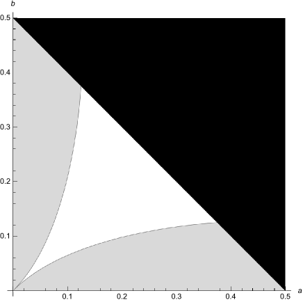
In view of Theorem 1.1, the condition $a+b\leq 1/2$ in Corollary 1.3 is necessary for the convexity of the function ${{}_{2}F_{1}}(a+1,b;1;z)/{{}_{2}F_{1}}(a,b;1;z)$ in the range $a+b<2.$ The picture in Figure 1 was produced by Mathematica based on Theorems 1.1 and 1.2. Note that the white region does not necessarily mean $\kappa[a,b,1]\leq 0.$

Putting $a=2-2\alpha$ and $b=2-2\beta$ in Corollary 1.3, we arrive at the following result solving partially the problem of Küstner which is mentioned above.

This section is devoted to some results on hypergeometric functions which will be used in the proof of main theorems. Formulas concerning the hypergeometric functions without specific references below can be found in [1] and [5].

A sequence $\{a_{n}\}_{n=0}^{\infty}$ of real numbers is called totally monotone or completely monotone if $\Delta^{k}a_{n}\geq 0$ for all integers $n,k\geq 0.$ Here, $\Delta^{k}a_{n}$ is defined recursively by $\Delta^{0}a_{n}=a_{n},n\geq 0,$ and $\Delta^{k}a_{n}=\Delta^{k-1}a_{n}-\Delta^{k-1}a_{n+1}$ for $n\geq 0$ and $k\geq 1.$

The following lemma is useful for our aim (see Theorems 69.2 and 71.1 in [10]).

We denote by ${\mathcal{T}}$ the class of functions $h\in{\operatorname{Hol}}({\mathbb{D}})$ with $h(0)>0$ satisfying one (and hence all) of the above three conditions. In what follows, we write

It is easily seen that $s_{1}h_{1}+s_{2}h_{2}\in{\mathcal{T}}$ for $s_{1},s_{2}\in(0,+\infty)$ and $h_{1},h_{2}\in{\mathcal{T}}.$ Note that a function $h\in{\mathcal{T}}$ can be analytically continued on the domain $\Lambda={\mathbb{C}}\setminus[1,+\infty)$ by using the integral representation in condition (ii). Therefore, we can regard ${\mathcal{T}}$ as a subset of ${\operatorname{Hol}}(\Lambda).$ Let ${\widetilde{\mathcal{T}}}$ be the class of functions $f\in{\operatorname{Hol}}(\Lambda)$ of the form $f(z)=zh(z)$ for some $h\in{\mathcal{T}}.$ Since the sequence $a_{1},a_{2},\dots$ is totally monotone for a totally monotone sequence $a_{0},a_{1},\dots,$ the function $h-h(0)$ belongs to ${\widetilde{\mathcal{T}}}$ for $h\in{\mathcal{T}},$ provided that $h^{\prime}(0)\neq 0.$ Geometric properties of functions $f\in{\widetilde{\mathcal{T}}}$ are investigated by many authors (see [4], [7] and [13] for instance). Among others, Wirths [13] showed that a function $f$ in ${\widetilde{\mathcal{T}}}$ maps both the half-plane ${\,\operatorname{Re}\,}z<1$ and the unit disk $|z|<1$ univalently onto domains convex in the direction of the imaginary axis (see also [2, Lem. 3.1]). Küstner [2] studied hypergeometric functions in connection with the class ${\widetilde{\mathcal{T}}}.$ Especially, the following result is important in the present work.

In particular, we note $g_{1}=b/c$ and $g_{2}=(a+1)/(c+1).$ We need also a few more results on continued fractions.

This estimate is simple and useful but it does not work for a function of the form in condition (iii) of Lemma 2.2 with $g_{0}=0.$ We offer a variant of the above estimate as follows.

The above inequality means that the value $h(z)=a_{0}+a_{1}z+a_{2}z^{2}+\cdots$ lies in the closed disk centered at $(h(1^{-})+h(-1))/2=\sum_{0}^{\infty}a_{2n}$ with radius $(h(1^{-})-h(-1))/2=\sum_{0}^{\infty}a_{2n+1}.$ This refines the obvious estimate $h(-1)\leq{\,\operatorname{Re}\,}h(z)\leq h(1^{-})$ for $z\in{\mathbb{D}}.$ When $h$ is not a constant, we can exclude the equality case, by the maximum modulus principle.

We note here transformations of continued fractions.

Applying the above lemmas, we have the following result.

Recall $g_{1}=b/c$ in (2.2). Applying Lemma 2.4 to the functions $T$ and $U,$ we obtain the following.

By the form of $T(z)$ in Lemma 2.7, we have $T(-1)=g_{1}/(1+(1-g_{1})g_{2}/(1+\ddots))\leq g_{1}=b/c.$ Using the relation $w(z)=1/(1-zT(z)),$ we have the following result ([11, Lem. 2.2], see also [12, Lem. 2.5]).

We also need the following information about the asymptotic behavior of $w(z)$ as $z\to 1.$