This paper was converted on www.awesomepapers.org from LaTeX by an anonymous user.
Want to know more? Visit the Converter page.

On Hypothesis Transfer Learning of Functional Linear Models

Haotian Lin Department of Statistics, The Pennsylvania State University Matthew Reimherr Department of Statistics, The Pennsylvania State University Amazon Science
Abstract

We study the transfer learning (TL) for the functional linear regression (FLR) under the Reproducing Kernel Hilbert Space (RKHS) framework, observing the TL techniques in existing high-dimensional linear regression is not compatible with the truncation-based FLR methods as functional data are intrinsically infinite-dimensional and generated by smooth underlying processes. We measure the similarity across tasks using RKHS distance, allowing the type of information being transferred tied to the properties of the imposed RKHS. Building on the hypothesis offset transfer learning paradigm, two algorithms are proposed: one conducts the transfer when positive sources are known, while the other leverages aggregation techniques to achieve robust transfer without prior information about the sources. We establish lower bounds for this learning problem and show the proposed algorithms enjoy a matching asymptotic upper bound. These analyses provide statistical insights into factors that contribute to the dynamics of the transfer. We also extend the results to functional generalized linear models. The effectiveness of the proposed algorithms is demonstrated on extensive synthetic data as well as a financial data application.

1 Introduction

Advances in technologies enable us to collect and process densely observed data over some temporal or spatial domains, which are coined functional data [Ramsay et al., 2005; Kokoszka and Reimherr, 2017]. While functional data analysis (FDA) has been proven useful in various fields like finance, genetics and etc., and has been researched widely in the statistical community, its effectiveness relies on having sufficient training samples drawn from the same distribution. However, this may not hold for functional data under some applications due to collection expenses or other constraints. Transfer learning (TL)[Torrey and Shavlik, 2010] leverages additional information from some similar (source) tasks to enhance the learning procedure on the original (target) task, and is an appealing mechanism when there is a lack of training samples. The goal of this paper is to develop TL algorithms for functional linear regression (FLR), one of the most prevalent models in the FDA. The FLR concerned in this paper is Scalar-on-Function regression, which takes the form:

Y=α+β,XL2+ϵ=α+𝒯X(s)β(s)𝑑s+ϵ,Y=\alpha+\langle\beta,X\rangle_{L^{2}}+\epsilon=\alpha+\int_{\mathcal{T}}X(s)\beta(s)\ ds+\epsilon,

where YY is a scalar response, X:𝒯X:\mathcal{T}\to\mathbb{R} and β:𝒯\beta:\mathcal{T}\to\mathbb{R} are the square-integrable functional predictor and coefficient function respectively over a compact domain 𝒯\mathcal{T}\subset\mathbb{R}, and ϵ\epsilon is a random noise with zero mean.

A classical approach to estimating β\beta is to reduce the problem to classical multivariate linear regression by expanding the XX and β\beta under the same finite basis, like deterministic basis functions, e.g. Fourier basis, or the eigenbasis of the covariance function of XX [Cardot et al., 1999; Yao et al., 2005; Hall and Hosseini-Nasab, 2006; Hall and Horowitz, 2007], which we refer to truncation-based FLR in this paper. Conceptually, the offset transfer learning techniques developed in multivariate/high-dimensional linear regression [Kuzborskij and Orabona, 2013, 2017; Li et al., 2022; Bastani, 2021] can be applied to truncation-based FLR methods, though they lack a theoretical foundation in this context due to the truncation error inherent in a basis expansion of β\beta. In particular, a key property distinguishing functional data from multivariate data is that they are inherently infinite-dimensional and generated through smooth underlying processes. Omitting this fact and treating the finite coefficients as multivariate parameters loses the benefit that data are generated from smooth processes, see detailed discussion in Section 2. Observing these limitations we develop the first TL algorithms for FLR with statistical risk guarantees under the supervised learning setting.

We summarize our main contributions as follows.

  1. 1.

    We propose using the Reproducing Kernel Hilbert Space (RKHS) distance between tasks’ coefficients as a measure of task similarity. The transferred information is thus tied to the RKHS’s properties and makes the transfer more interpretable. One can tailor the employed RKHS to the task’s nature, offering flexibility to embed diverse structural elements, like smoothness or periodicity, into TL processes.

  2. 2.

    Built upon the offset transfer learning (OTL) paradigm, we propose TL-FLR, a variant of OTL for multiple positive transfer sources. We establish the minimax optimality for TL-FLR. Intriguingly, the result reveals that the faster statistical rate of TL-FLR, compared to non-transfer learning, not only depends on source sample size and the magnitude of discrepancy across tasks like most existing works, but also the signal ratio between offset and source model.

  3. 3.

    To deal with the practical scenario in which there is no available prior task similarity information, we propose Aggregation-based TL-FLR (ATL-FLR), utilizing sparse aggregation to mitigate negative transfer effects. We establish the upper bound for ATL-FLR and show the aggregation cost decreases faster than the transfer learning risk, demonstrating an ability to identify optimal sources without too much extra cost compared to TL-FLR. We further extend this framework to Functional Generalized Linear Models (FGLM) with theoretical guarantees, broadening its applicability.

  4. 4.

    In developing statistical guarantees, we uncovered unique requirements for making OTL theoretically feasible in the functional data context. These include the necessity for covariate functions across tasks to exhibit similar structural properties to ensure statistical convergence, and the coefficient functions of negative sources can be separated from positive ones within a finite-dimensional space to ensure optimal source identification.

Literature review.

Apart from truncation-based FLR approaches mentioned before, another line of research proposed that one can obtain a smooth estimator, via smoothness regularization [Yuan and Cai, 2010; Cai and Yuan, 2012], and has been widely used in other functional models like the FGLM, functional Cox-model, etc. [Cheng and Shang, 2015; Qu et al., 2016; Reimherr et al., 2018; Sun et al., 2018].

Turning to the TL regime in supervised learning, the hypothesis transfer learning (HTL) framework has become popular [Li and Bilmes, 2007; Orabona et al., 2009; Kuzborskij and Orabona, 2013; Perrot and Habrard, 2015; Du et al., 2017]. Offset transfer learning (OTL) (a.k.a. biases regularization transfer learning) has been widely analyzed and applied as one of the most popular HTL paradigms. It assumes the target’s function/parameter is a summation of the source’s and the offset’s function/parameter. A series of works have derived theoretical analysis under different settings. For example, in Kuzborskij and Orabona [2013, 2017], the authors provide the first theoretical study of OTL in the context of linear regression with stability analysis and generalization bounds. Later, in Wang and Schneider [2015]; Wang et al. [2016] the authors derive similar theoretical guarantees for non-parametric regression via Kernel Ridge Regression. A unified framework that generalizes many previous works is proposed in Du et al. [2017] and the authors also present an excess risk analysis for their framework. Apart from the regression setting, generalization bounds for classification with surrogate losses have been studied in Aghbalou and Staerman [2023]. Other results that study HTL outside OTL can be found in Li and Bilmes [2007]; Cheng and Shang [2015]. Besides, OTL can also be viewed as a case of representation learning [Du et al., 2020; Tripuraneni et al., 2020; Xu and Tewari, 2021] by viewing the estimated source model as a representation for target tasks.

OTL has recently been adopted by the statistics community for various high-dimensional models with statistical risk guarantees. For example, Bastani [2021] proposed using OTL for high-dimensional (generalized) linear regression but only includes one positive transfer source. Later, Li et al. [2022] extended this idea to multiple sources scenario and leveraged aggregation to alleviate negative transfer effects. In Tian and Feng [2022], the learning procedure gets extended to the high-dimensional generalized linear model and the authors also proposed a positive sources detection algorithm via a validation approach. In these works, the similarity among tasks is quantified via 1\ell^{1}-norm, which captures the sparsity structure in high-dimensional parameters. There is no TL for FDA that we are aware of, but the closest work would be in the area of domain adaptation. Zhu et al. [2021] studied the domain adaptation problem between two separable Hilbert spaces by proposing algorithms to estimate the optimal transport mapping between two spaces.

Notation.

For two sequence {ak}k1\{a_{k}\}_{k\geq 1} and {bk}k1\{b_{k}\}_{k\geq 1}, we denotes anbna_{n}\asymp b_{n} and anbna_{n}\lesssim b_{n} if |an/bn|c|a_{n}/b_{n}|\rightarrow c and |an/bn|c|a_{n}/b_{n}|\leq c for some universal constant cc when nn\rightarrow\infty. For two random variable sequence {Ak}k1\{A_{k}\}_{k\geq 1} and {Bk}k1\{B_{k}\}_{k\geq 1}, if for any δ>0\delta>0, there exists Mδ>0M_{\delta}>0 and Nδ>0N_{\delta}>0 such that (Ak<MδBk)1δ\mathbb{P}(A_{k}<M_{\delta}B_{k})\geq 1-\delta, kNδ\forall k\geq N_{\delta}, we say Ak=O(Bk)A_{k}=O_{\mathbb{P}}(B_{k}). For a set AA, let |A||A| denote its cardinality, AcA^{c} denote its complement. For an integer nn, denote [n]:={1,,n}[n]:=\{1,\cdots,n\}.

We denote the covariance function of XX as C(s,t)=E[X(s)EX(s)][X(t)EX(t)]C(s,t)=\operatorname{E}[X(s)-\operatorname{E}X(s)][X(t)-\operatorname{E}X(t)] for s,t𝒯s,t\in\mathcal{T}. For a real, symmetric, square-integrable, and nonnegative kernel, K:𝒯×𝒯K:\mathcal{T}\times\mathcal{T}\rightarrow\mathbb{R}, we denote its associated RKHS on 𝒯\mathcal{T} as K\mathcal{H}_{K} and corresponding norm as K\|\cdot\|_{K}. We also denote its integral operator as LK(f)=𝒯K(,t)f(t)𝑑tL_{K}(f)=\int_{\mathcal{T}}K(\cdot,t)f(t)dt\quad for fL2f\in L^{2}. For two kernels, K1K_{1} and K2K_{2}, their composition is (K1K2)(s,t)=𝒯K1(s,u)K2(u,t)𝑑u(K_{1}K_{2})(s,t)=\int_{\mathcal{T}}K_{1}(s,u)K_{2}(u,t)du. For a given kernel KK and covariance kernel CC, define bivariate function Γ\Gamma and its integral operator as Γ:=K1/2CK1/2\Gamma:=K^{1/2}CK^{1/2} and LΓ(f)=LK12(LC(LK12(f)))L_{\Gamma}(f)=L_{K^{\frac{1}{2}}}(L_{C}(L_{K^{\frac{1}{2}}}(f))).

2 Preliminaries and Backgrounds

Problem Set-up.

We now formally set the stage for the transfer learning problem in the context of FLR. Consider the following series of FLRs,

Yi(t)=α(t)+Xi(t),β(t)L2+ϵi(t)Y_{i}^{(t)}=\alpha^{(t)}+\left\langle X_{i}^{(t)},\beta^{(t)}\right\rangle_{L^{2}}+\epsilon_{i}^{(t)} (1)

for i[nt]i\in[n_{t}], t=0[T]t=0\cup[T], where t=0t=0 denotes the target model and t[T]t\in[T] denotes source models. Denote the sample space 𝒵\mathcal{Z} as the Cartesian product of the covariate space 𝒳\mathcal{X} and response space 𝒴\mathcal{Y}. For each t0[T]t\in 0\cup[T], we denote 𝒟(t)={(Xi(t),Yi(t))}i=1nt={Zi(t)}i=1nt\mathcal{D}^{(t)}=\{(X_{i}^{(t)},Y_{i}^{(t)})\}_{i=1}^{n_{t}}=\{Z_{i}^{(t)}\}_{i=1}^{n_{t}}. Throughout the paper we assume ϵi(t)\epsilon_{i}^{(t)} are i.i.d. across both ii and tt with zero mean and finite variance σ2\sigma^{2}.

As estimating β(0)\beta^{(0)} is our primary interest, we assume for simplicity that α(t)=0\alpha^{(t)}=0 for all tt. We assume n0l=1Tntn_{0}\ll\sum_{l=1}^{T}n_{t}, a condition commonly validated in most TL literature and numerous practical applications. While our framework is designed primarily for the posterior drift setting, i.e. the marginal distributions of X(t)X^{(t)} remain the same but β(t)\beta^{(t)} vary, the excess risk bounds we establish are based on a comparatively more relaxed condition, see Section 4.

In the absence of source data, estimating β(0)\beta^{(0)} is termed as target-only learning and one can obtain a smooth estimator of β\beta through the regularized empirical risk minimization (RERM) [Yuan and Cai, 2010; Cai and Yuan, 2012], i.e.

β^=argminβK{1n0i=1n0(β,Zi(0))+λβK2},\hat{\beta}=\underset{\beta\in\mathcal{H}_{K}}{\operatorname{argmin}}\left\{\frac{1}{n_{0}}\sum_{i=1}^{n_{0}}\ell(\beta,Z_{i}^{(0)})+\lambda\|\beta\|_{K}^{2}\right\},

where KK is an employed kernel and :K×𝒵+\ell:\mathcal{H}_{K}\times\mathcal{Z}\rightarrow\mathbb{R}^{+} is the loss function. This approach has been proven to achieve the optimal rate in terms of excess risk, and we refer to it as Optimal Functional Linear Regression (OFLR) in this paper, which serves as a non-transfer learning baseline.

Similarity Measure.

We first state the limitations of using 1/2\ell^{1}/\ell^{2}-norm as a similarity measure in the truncation-based FLR method, which converts the problem into a classic multivariate one. For a given series of basis functions {ϕj}j1\{\phi_{j}\}_{j\geq 1} and truncated number MM, one can model the tt-th FLR as

Yi(t)j=1MXij(t)βj(t)+ϵi(t)Y_{i}^{(t)}\approx\sum_{j=1}^{M}X_{ij}^{(t)}\beta_{j}^{(t)}+\epsilon_{i}^{(t)} (2)

where Xij(t)=Xi(t),ϕjL2X_{ij}^{(t)}=\langle X_{i}^{(t)},\phi_{j}\rangle_{L^{2}} and βj(t)=β(t),ϕjL2\beta_{j}^{(t)}=\langle\beta^{(t)},\phi_{j}\rangle_{L^{2}}. Denote βtrunc(t)M\beta^{(t)}_{\text{trunc}}\in\mathbb{R}^{M} as the coefficient vector in (2), one can then measure the similarity between the target and the tt-th FLR model by the 1\ell^{1} or 2\ell^{2} norm of βtrunc(t)βtrunc(0)\beta^{(t)}_{\text{trunc}}-\beta^{(0)}_{\text{trunc}} like the previous works did for multivariate linear regression. However, from the functional data analysis literature, since the functional data are generated from some structural underlying process, it is well known that one has to have the same kind of structure in the estimator like smoothness for theoretical reliability. For example, when the coefficient functions are smooth, the above approach cannot measure the similarity, since {βtrunc(t)}t=0T\{\beta^{(t)}_{\text{trunc}}\}_{t=0}^{T} are not necessarily sparse or might require regularization via an 2\ell^{2}-norm, but the employed basis functions might not reflect the desired smoothness. Besides, the basis functions and MM should be consistent across tasks, which reduces the flexibility of the learning procedure.

To explore the similarity tied to the structure of coefficient functions, one should quantify the similarity between tasks within certain functional spaces that possess the same structures. These structural properties, e.g. continuity/smoothness/periodicity, can be naturally encapsulated via kernels and their corresponding RKHS. Consequently, quantifying the similarity within a certain RKHS provides interpretability since the type of information transferred is tied to the structural properties of the used RKHS. We also note that this method is broadly applicable since the reproducing kernel can be tailored to the application problem accordingly. For example, one can transfer the information about continuity or smoothness by picking KK to be a Sobolev kernel, and about periodicity by picking periodic kernels like K(x1,x2)=exp(2/l2sin(π|x1x2|/p))K(x_{1},x_{2})=exp\left(-2/l^{2}\sin\left(\pi|x_{1}-x_{2}|/p\right)\right) where ll is the lengthscale and pp is the period.

Given the reasoning above, for t=0[T]t=0\cup[T], we assume β(t)K\beta^{(t)}\in\mathcal{H}_{K}, and define the tt-th contrast function δ(t):=β(0)β(t)\delta^{(t)}:=\beta^{(0)}-\beta^{(t)}. Given a constant h0h\geq 0, we say the tt-th source model is “h-transferable” if δ(t)Kh\|\delta^{(t)}\|_{K}\leq h. The magnitude of hh characterizes the similarity between the target model and source models. We also define 𝒮h={t[T]:δ(t)Kh}\mathcal{S}_{h}=\{t\in[T]:\|\delta^{(t)}\|_{K}\leq h\} as a subset of [T][T], which consists of the indexes of all “h-transferable” source models. It is worth mentioning that the quantity hh is introduced for theoretical purposes to establish optimality, which is prevalent in recent studies such as Bastani [2021]; Cai and Wei [2021]. But for the implementation of the algorithm, it is not necessary to know the actual value of hh. We abbreviate 𝒮h\mathcal{S}_{h} as 𝒮\mathcal{S} to generally represent the h-transferable sources index.

Learning Framework.

This paper leverages the widely used OTL paradigm, see reviews in Section 1. Formally, in the FLR and single source β(1)\beta^{(1)} context, the OTL obtains the target function via β^(0)=β^(1)+δ^\hat{\beta}^{(0)}=\hat{\beta}^{(1)}+\hat{\delta} where β^(1)\hat{\beta}^{(1)} is the estimator trained on source dataset and δ^\hat{\delta} is obtained from target dataset via following minimization problem:

δ^=argminδK1n0i=1n0(δ+β^(0),Zi(0))+λδK2,\hat{\delta}=\underset{\delta\in\mathcal{H}_{K}}{\operatorname{argmin}}\frac{1}{n_{0}}\sum_{i=1}^{n_{0}}\ell(\delta+\hat{\beta}^{(0)},Z_{i}^{(0)})+\lambda\|\delta\|_{K}^{2},

where the loss function can be square loss [Orabona et al., 2009; Kuzborskij and Orabona, 2013] or surrogate losses [Aghbalou and Staerman, 2023]. The main idea is that the estimator β^(1)\hat{\beta}^{(1)} can be learned well given sufficiently large source samples and the simple offset estimator δ^(0)\hat{\delta}^{(0)} can be learned with much fewer target samples.

3 Methodology

3.1 Transfer Learning with 𝒮\mathcal{S} Known

For multiple sources, the idea of data fusion inspires us to obtain a centered source estimator β𝒮\beta_{\mathcal{S}} via all source datasets in place of β(1)\beta^{(1)}. Therefore, we can generalize single source OTL to the multiple sources scenario as follows.

Algorithm 1 TL-FLR
1:Input: Target/Source datasets {𝒟(t)}t=0T\{\mathcal{D}^{(t)}\}_{t=0}^{T}; index set of source datasets 𝒮\mathcal{S}; Loss function \ell as square loss.
2:
3:Transfer Step: Obtain β^𝒮\hat{\beta}_{\mathcal{S}} via
β^𝒮=argminβKt𝒮1nti=1nt(β,Zi(t))+λ1βK2.\hat{\beta}_{\mathcal{S}}=\underset{\beta\in\mathcal{H}_{K}}{\operatorname{argmin}}\sum_{t\in\mathcal{S}}\frac{1}{n_{t}}\sum_{i=1}^{n_{t}}\ell(\beta,Z_{i}^{(t)})+\lambda_{1}\|\beta\|_{K}^{2}. (3)
4:Calibration Step: Obtain offset δ^\hat{\delta} via
δ^=argminδK1n0i=1n0(δ+β^𝒮,Zi(0))+λ2δK2.\hat{\delta}=\underset{\delta\in\mathcal{H}_{K}}{\operatorname{argmin}}\frac{1}{n_{0}}\sum_{i=1}^{n_{0}}\ell(\delta+\hat{\beta}_{\mathcal{S}},Z_{i}^{(0)})+\lambda_{2}\|\delta\|_{K}^{2}. (4)
5:Return β^S+δ^\hat{\beta}_{S}+\hat{\delta}.

Since the probabilistic limit of β^𝒮\hat{\beta}_{\mathcal{S}} is not consistent with β(0)\beta^{(0)}, calibration of β^𝒮\hat{\beta}_{\mathcal{S}} is performed in (4). The regularization term in (4) is consistent with our similarity measure, i.e. it restricts β^(0)\hat{\beta}^{(0)} to lie in a K\mathcal{H}_{K} ball centered at β^𝒮\hat{\beta}_{\mathcal{S}}. Therefore, this term pushes the β^(0)\hat{\beta}^{(0)} close to β^𝒮\hat{\beta}_{\mathcal{S}} while the mean square error loss over the target dataset allows calibration for the bias. Intuitively, if β^𝒮\hat{\beta}_{\mathcal{S}} is close to β(0)\beta^{(0)} then TL-FLR can boost the learning on the target model.

3.2 Transfer Learning with Unknown 𝒮\mathcal{S}

Assuming the index set 𝒮\mathcal{S} is known in Algorithm 1 can be unrealistic in practice without prior information or investigation. Moreover, as some source tasks might have little or even a negative contribution to the target one, it could be practically harmful to directly apply Algorithm 1 by assuming all sources belong to 𝒮\mathcal{S}. Inspired by the idea of aggregating multiple estimators in Li et al. [2022], we develop ATL-FLR which can be directly applied without knowing 𝒮\mathcal{S} while being robust to negative transfer sources.

The general idea of ATL-FLR is that one can first construct a collection of candidates for 𝒮\mathcal{S}, named {𝒮1^,𝒮2^,,𝒮J^}\{\hat{\mathcal{S}_{1}},\hat{\mathcal{S}_{2}},\cdots,\hat{\mathcal{S}_{J}}\}, such that there exists at least one 𝒮^j\hat{\mathcal{S}}_{j} satisfying 𝒮^j=𝒮\hat{\mathcal{S}}_{j}=\mathcal{S} with high probability and then obtain their corresponding estimators ={β^(𝒮1^),,β^(𝒮J^)}\mathcal{F}=\{\hat{\beta}(\hat{\mathcal{S}_{1}}),\cdots,\hat{\beta}(\hat{\mathcal{S}_{J}})\} via TL-FLR. Then, one aggregates the candidate estimators in \mathcal{F} such that the aggregated estimator β^a\hat{\beta}_{a} satisfies the following oracle inequality in high probability,

R(β^a)minβR(β)+r(,n),R(\hat{\beta}_{a})\leq\min_{\beta\in\mathcal{F}}R(\beta)+r(\mathcal{F},n), (5)

where R(f)=E(X,Y)[(Y,f(X))|{𝒟(t):t0[T]}]\quad R(f)=\operatorname{E}_{(X,Y)}[\ell(Y,f(X))|\{\mathcal{D}^{(t)}:t\in 0\cup[T]\}], and r(,n)r(\mathcal{F},n) is the aggregation cost. Thus the β^a\hat{\beta}_{a} can achieve similar performance as TL-FLR up to some aggregation cost. Formally, the proposed aggregation-based TL-FLR is as follows.

Algorithm 2 Aggregation-based TL-FLR (ATL-FLR)
Input: Target/Source datasets {𝒟(t))}t=0T\{\mathcal{D}^{(t))}\}_{t=0}^{T}; index set of source datasets 𝒮\mathcal{S}; Loss function \ell as square loss; A given integer MM.
Step 1: Split the target dataset 𝒟(0)\mathcal{D}^{(0)} into 𝒟(0)\mathcal{D}_{\mathcal{I}}^{(0)} and 𝒟c(0)\mathcal{D}_{\mathcal{I}^{c}}^{(0)} with \mathcal{I} be a random subset of [n0][n_{0}] such that ||=n02|\mathcal{I}|=\lfloor\frac{n_{0}}{2}\rfloor.
Step 2: Built candidate sets of 𝒮\mathcal{S}, {𝒮^0,𝒮^1,,𝒮^T}\{\hat{\mathcal{S}}_{0},\hat{\mathcal{S}}_{1},\cdots,\hat{\mathcal{S}}_{T}\} as:
  1. 1.

    Obtain β^0\hat{\beta}_{0} by OFLR using 𝒟(0)\mathcal{D}_{\mathcal{I}}^{(0)} and let 𝒮^0=\hat{\mathcal{S}}_{0}=\emptyset.

  2. 2.

    For each t[T]t\in[T], obtain β^t\hat{\beta}_{t} by OFLR using 𝒟(t)\mathcal{D}^{(t)} and obtain truncated RKHS norm Δ^t=β^0β^tKM:=j=1Mβ^0β^t,vj2/τj\hat{\Delta}_{t}=\|\hat{\beta}_{0}-\hat{\beta}_{t}\|_{K^{M}}:=\sum_{j=1}^{M}\langle\hat{\beta}_{0}-\hat{\beta}_{t},v_{j}\rangle^{2}/\tau_{j}.

  3. 3.

    Set 𝒮^t={k[T]:Δ^k is among the first t smallest.}\hat{\mathcal{S}}_{t}=\left\{k\in[T]:\hat{\Delta}_{k}\text{ is among the first }t\text{ smallest.}\right\}

Step 3: For t[T]t\in[T], fit TL-FLR by setting 𝒮=𝒮^t\mathcal{S}=\hat{\mathcal{S}}_{t} with dataset 𝒟(0)\mathcal{D}_{\mathcal{I}}^{(0)}. Let ={β^(𝒮^0),β^(𝒮^1),β^(𝒮^T)}\mathcal{F}=\{\hat{\beta}(\hat{\mathcal{S}}_{0}),\hat{\beta}(\hat{\mathcal{S}}_{1}),\cdots\hat{\beta}(\hat{\mathcal{S}}_{T})\}.
Step 4: Implement the sparse aggregation procedure in Algoritm 3 with \mathcal{F} as the dictionary and training dataset as 𝒟c(0)\mathcal{D}_{\mathcal{I}^{c}}^{(0)}. Obtain the sparse aggregated estimator β^a\hat{\beta}_{a}.
Remark 1.

While exploring the estimated similarity across sources to the target in Step 2, we use a truncated RKHS norm, which is the distance between β^0\hat{\beta}_{0} and β^t\hat{\beta}_{t} after projecting them onto the space spanned by the first MM eigenfunctions of KK. Here, {τj}j1\{\tau_{j}\}_{j\geq 1} and {vj}j1\{v_{j}\}_{j\geq 1} are the eigenvalues and eigenfunctions of KK. Such a truncated norm guarantees the identifiability of 𝒮\mathcal{S}, see Section 4.2 for detail.

Step 2 ensures the target-only baseline β^0\hat{\beta}_{0} lies in \mathcal{F} while the construction of 𝒮^t\hat{\mathcal{S}}_{t} ensures thorough exploration of 𝒮\mathcal{S}. If 𝒮\mathcal{S} can be identified by one of the 𝒮^t\hat{\mathcal{S}}_{t}, then inequality (5) indicates that even without knowing 𝒮\mathcal{S}, the β^a\hat{\beta}_{a} can mimic the performance of the TL-FLR estimator, while not being worse than the target-only β^0\hat{\beta}_{0}, up to an aggregation cost.

The sparse aggregation is adopted from Gaîffas and Lecué [2011], see Appendix B. Although we note that other aggregation methods like aggregate with cumulated exponential weights (ACEW) [Juditsky et al., 2008; Audibert, 2009], aggregate with exponential weights (AEW) [Leung and Barron, 2006; Dalalyan and Tsybakov, 2007], and Q-aggregation [Dai et al., 2012] can replace sparse aggregation in Step 4, sparse aggregation is often preferred due to its computational efficiency and ability to eliminate negative transfer effects. Specifically, the final aggregated estimator is usually represented as a convex combination of elements in \mathcal{F} i.e. β^a=j=1Jcjβ^(𝒮^j)\hat{\beta}_{a}=\sum_{j=1}^{J}c_{j}\hat{\beta}(\hat{\mathcal{S}}_{j}). The sparse aggregation sets most of the cjc_{j} to zero, which effectively excludes the negative transfer sources. On the other hand, none of the ACEW, AEW, and Q-aggregation will set the cjc_{j} to 0 most of the time, meaning that negative transfer sources can still affect β^a\hat{\beta}_{a}. Although one can manually tune temperature parameters in these approaches to shrink the cjc_{j} close to zero, they are less computationally efficient given the fact that sparse aggregation does not require such a tuning process. In Section 6, we verify that sparse aggregation outperforms other aggregation methods under various settings.

4 Theoretical Analysis

In this section, we study the theoretical properties of the prediction accuracy of the proposed algorithms. We evaluate the proposed algorithms via excess risk, i.e.

(β^(0)):=EZ(0)[(β^(0),Z(0))(β(0),Z(0))]\mathcal{E}(\hat{\beta}^{(0)}):=\operatorname{E}_{Z^{(0)}}\left[\ell(\hat{\beta}^{(0)},Z^{(0)})-\ell(\beta^{(0)},Z^{(0)})\right]

where the expectation is taken over an independent test data point Z(0)Z^{(0)} from the target distribution. To study the excess risk of TL-FLR and ATL-FLR, we define the parameter space as

Θ(h)={(β(0),{β(t)}t𝒮):maxt𝒮δ(t)Kh}.\Theta(h)=\left\{\left(\beta^{(0)},\{\beta^{(t)}\}_{t\in\mathcal{S}}\right):\max_{t\in\mathcal{S}}\|\delta^{(t)}\|_{K}\leq h\right\}.

To establish the theoretical analysis of the proposed algorithms, we first state some assumptions. For t0[T]t\in 0\cup[T], denote {sj(t)}j1\{s_{j}^{(t)}\}_{j\geq 1} and {ϕj(t)}j1\{\phi_{j}^{(t)}\}_{j\geq 1} as the eigenvalues and eigenfunctions of Γ(t):=K12C(t)K12\Gamma^{(t)}:=K^{\frac{1}{2}}C^{(t)}K^{\frac{1}{2}} respectively.

Assumption 1 (Eigenvalue Decay Rate (EDR)).

Suppose that the eigenvalue decay rate (EDR) of LΓ(0)L_{\Gamma^{(0)}} is 2r2r, i.e.

sj(0)j2r,j1.s_{j}^{(0)}\asymp j^{-2r},\quad\forall j\geq 1.

The polynomial EDR assumption is standard in FLR literature like Cai and Yuan [2012]; Reimherr et al. [2018]. RKHSs that satisfy this assumption, like Sobolev spaces, are natural choices when one is concerned about the smoothness being the structural properties in the TL processes.

Assumption 2.

We assume either one of the following conditions holds.

  1. 1.

    LΓ(t)L_{\Gamma^{(t)}} commutes with LΓ(0)L_{\Gamma^{(0)}}, t𝒮\forall t\in\mathcal{S}, i.e. LΓ(0)LΓ(t)=LΓ(t)LΓ(0)L_{\Gamma^{(0)}}L_{\Gamma^{(t)}}=L_{\Gamma^{(t)}}L_{\Gamma^{(0)}}, and

    aj(t):=LΓ(t)(ϕj(0)),ϕj(0)sj(0)j1.a_{j}^{(t)}:=\langle L_{\Gamma^{(t)}}(\phi_{j}^{(0)}),\phi_{j}^{(0)}\rangle\asymp s_{j}^{(0)}\quad\forall j\geq 1.
  2. 2.

    Or the following linear operator is Hilbert–Schmidt.

    𝐈(LΓ(0))1/2LΓ(t)(LΓ(0))1/2,t𝒮.\mathbf{I}-(L_{\Gamma^{(0)}})^{-1/2}L_{\Gamma^{(t)}}(L_{\Gamma^{(0)}})^{-1/2},\quad\forall t\in\mathcal{S}.

We note that under the posterior drift setting, both conditions in Assumption 2 are satisfied automatically. Although neither condition implies the other, both conditions primarily focus on how the smoothness of the source kernel Γ(t)\Gamma^{(t)} relates to that of the target kernel Γ(0)\Gamma^{(0)}. Specifically, Condition 1 implies LΓ(0)L_{\Gamma^{(0)}} and LΓ(t)L_{\Gamma^{(t)}} not only share the same eigenspace but also have similar magnitudes of the projection onto the jj-th dimension of the eigenspace, which commonly appears in FDA literature [Yuan and Cai, 2010; Balasubramanian et al., 2022]. This helps us to control the excess risk of β^S\hat{\beta}_{S} over the target domain. Condition 2 implies the probability measures of X(0)X^{(0)} and X(t)X^{(t)} are equivalent, see Baker [1973]. Collectively, these conditions indicate the feasibility of OTL for functional data relies on the fact that source covariance function C(t)C^{(t)} should behave similarly to the target’s C(0)C^{(0)}. Either a too “smooth” or a too “rough” X(t)X^{(t)} can degrade the optimality. This aligns with the principles of standard target-only FLR, where the performance of the estimator is jointly determined by the covariance function and reproducing kernel.

4.1 Minimax Excess Risk of TL-FLR

We first provide the upper bound of excess risk on TL-FLR.

Theorem 1 (Upper Bound).

Suppose Assumption 2 and 1 hold. If n0/n𝒮0n_{0}/n_{\mathcal{S}}\nrightarrow 0, let ξ(h,𝒮)=h2β𝒮K2\xi(h,\mathcal{S})=\frac{h^{2}}{\|\beta_{\mathcal{S}}\|_{K}^{2}}, then for the output β^\hat{\beta} of Algorithm 1,

supΘ(h)(β^)=O(n𝒮2r2r+1+n02r2r+1ξ(h,𝒮)),\sup_{\Theta(h)}\mathcal{E}\left(\hat{\beta}\right)=O_{\mathbb{P}}\left(n_{\mathcal{S}}^{-\frac{2r}{2r+1}}+n_{0}^{-\frac{2r}{2r+1}}\xi(h,\mathcal{S})\right), (6)

if λ1n𝒮2r2r+1\lambda_{1}\asymp n_{\mathcal{S}}^{-\frac{2r}{2r+1}} and λ2n02r2r+1\lambda_{2}\asymp n_{0}^{-\frac{2r}{2r+1}} where λ1\lambda_{1} and λ2\lambda_{2} are regularization parameters in Algorithm 1.

Theorem 1 provides the excess risk upper bound of β^\hat{\beta}, which bounds the excess risk of two terms. The first term comes from the transfer step and depends on the sample size of sources in 𝒮\mathcal{S}, while the second term is due to only using the target dataset to learn the offset. In the trivial case when 𝒮=\mathcal{S}=\emptyset, the upper bound becomes O(n02r/(2r+1))O_{\mathbb{P}}(n_{0}^{-2r/(2r+1)}), which coincides with the upper bound of target-only baseline OFLR [Cai and Yuan, 2012]. When 𝒮\mathcal{S}\neq\emptyset, compared with the excess risk of the target-only baseline, we can see the sample size n𝒮n_{\mathcal{S}} in source models and the factor ξ(h,𝒮)\xi(h,\mathcal{S}) are jointly affecting the transfer learning. The factor ξ(h,𝒮)\xi(h,\mathcal{S}) represents the relative task signal strength between the source and target tasks. Geometrically, one can interpret ξ(h,fS)\xi(h,f_{S}) as the factor controlling the angle between the source and target models within the RKHS.
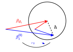
Refer to caption

Figure 1: Geometric illustration for how ξ(h,𝒮)\xi(h,\mathcal{S}) will affect the transfer dynamic. The circle represents an RKHS ball centered around β(0)\beta^{(0)} with radius hh. With the same hh, larger signal strength of β𝒮\beta_{\mathcal{S}}, i.e. β𝒮1K\|\beta_{\mathcal{S}_{1}}\|_{K} leads to smaller ξ(h,𝒮)\xi(h,\mathcal{S}), while smaller signal strength of β𝒮\beta_{\mathcal{S}}, i.e. β𝒮2K\|\beta_{\mathcal{S}_{2}}\|_{K} leads to larger ξ(h,𝒮)\xi(h,\mathcal{S}).

Figure 1 shows how n𝒮n_{\mathcal{S}} and ξ(h,𝒮)\xi(h,\mathcal{S}) impact the learning rate. When the βS\beta_{S} and β(0)\beta^{(0)} are more concordant (β𝒮1\beta_{\mathcal{S}_{1}} and β1(0)\beta_{1}^{(0)}), the angle between them are small and thus so the ξ(h,𝒮)\xi(h,\mathcal{S}), making the second term in the upper bound negligible in the excess risk, and thus the risk converges faster compared to baseline n02r/(2r+1)n_{0}^{-2r/(2r+1)} given sufficiently large n𝒮n_{\mathcal{S}}. If βS\beta_{S} and β(0)\beta^{(0)} are less concordant (β𝒮2\beta_{\mathcal{S}_{2}} and β2(0)\beta_{2}^{(0)}), leveraging β𝒮\beta_{\mathcal{S}} will be less effective since a large ξ(h,𝒮)\xi(h,\mathcal{S}) will make the second term the dominate term.

It is worth noting that most of the existing literature fails to identify how ξ(h,𝒮)\xi(h,\mathcal{S}) affects the effectiveness of OTL. For example, in Wang et al. [2016]; Du et al. [2017], this factor does not appear in the upper bound, and they claim nSn0n_{S}\gg n_{0} provide successful transfer from source to target. In high-dimensional linear regression [Li et al., 2022; Tian and Feng, 2022], the authors only identify ξ(h,𝒮)\xi(h,\mathcal{S}) is proportional to hh and claims a small hh can provide a faster convergence rate excess risk. However, our analysis (Figure 1) shows even with the same hh, the similarity of the two tasks can be different, since the signal strength of β𝒮\beta_{\mathcal{S}} will also affect the effectiveness of OTL. To this end, this reveals that one cannot obtain a faster excess risk in OTL by simply including more source datasets (larger n𝒮n_{\mathcal{S}}), but should also carefully select or construct the 𝒮\mathcal{S}.

Theorem 2 (Lower Bound).

Under the same condition of Theorem 1, for any possible estimator β~\tilde{\beta} based on {𝒟(t):t{0}𝒮}\{\mathcal{D}^{(t)}:t\in\left\{0\right\}\cup\mathcal{S}\}, the excess risk of β~\tilde{\beta} satisfies

lima0limninfβ~supΘ(h)P{(β~)a(n𝒮2r2r+1+n02r2r+1ξ(h,𝒮))}=1.\lim_{a\rightarrow 0}\lim_{n\rightarrow\infty}\inf_{\tilde{\beta}}\sup_{\Theta(h)}P\left\{\mathcal{E}\left(\tilde{\beta}\right)\geq a\left(n_{\mathcal{S}}^{-\frac{2r}{2r+1}}+n_{0}^{-\frac{2r}{2r+1}}\xi(h,\mathcal{S})\right)\right\}=1. (7)

Combining Theorems 1 and 2 implies that the estimator from TL-FLR is rate-optimal in excess risk. The proof of the lower bound is based on considering the lower bound of two cases: (1) the ideal case where β(t)=β(0)\beta^{(t)}=\beta^{(0)} for all t𝒮t\in\mathcal{S} and (2) the worst case where β(t)0\beta^{(t)}\equiv 0, meaning no knowledge should be transferred at all.

4.2 Excess Risk of ATL-FLR

In this subsection, we study the excess risk for ATL-FLR. As we discussed before, making ATL-FLR achieve similar performance to TL-FLR relies on the fact that there exists a 𝒮^t\hat{\mathcal{S}}_{t} such that it equals to the true 𝒮\mathcal{S} (so β^(𝒮^t)=β^(𝒮)\hat{\beta}(\hat{\mathcal{S}}_{t})=\hat{\beta}(\mathcal{S})) with high probability. Therefore, to ensure the \mathcal{F} constructed in Step 2 of Algorithm 2 satisfies such a property, we impose the following assumption to guarantee the identifiability of 𝒮\mathcal{S} and thus ensure the existence of such 𝒮^t\hat{\mathcal{S}}_{t}.

Assumption 3 (Identifiability of 𝒮\mathcal{S}).

Suppose for any hh, there is an integer MM such that

mint𝒮cβ0βtKM>h,\min_{t\in\mathcal{S}^{c}}\|\beta_{0}-\beta_{t}\|_{K^{M}}>h,

where KM\|\cdot\|_{K^{M}} is the truncated version of K\|\cdot\|_{K} defined in Algorithm 2.

Assumption 3 ensures that t𝒮c\forall t\in\mathcal{S}^{c}, there exists a finite-dimensional subspace of K\mathcal{H}_{K}, such that the norm of the projection of the contrast function, δ(t)\delta^{(t)}, on this subspace is already greater than hh. This assumption indeed eliminates the existence of β(t)\beta^{(t)}, for t𝒮ct\in\mathcal{S}^{c}, that live on the boundary of the RKHS-ball centered at β(0)\beta^{(0)} with radius hh in K\mathcal{H}_{K}. Under Assumption 3, we now show the \mathcal{F} constructed in Algorithm 2 guarantees the existence of 𝒮^t\hat{\mathcal{S}}_{t}.

Theorem 3.

Suppose Assumption 3 holds, then

maxt𝒮Δt<mint𝒮cΔtand(maxt𝒮Δ^t<mint𝒮cΔ^t)1,\max_{t\in\mathcal{S}}\Delta_{t}<\min_{t\in\mathcal{S}^{c}}\Delta_{t}\quad\text{and}\quad\mathbb{P}\left(\max_{t\in\mathcal{S}}\hat{\Delta}_{t}<\min_{t\in\mathcal{S}^{c}}\hat{\Delta}_{t}\right)\rightarrow 1,

and hence there exists a tt s.t. 𝒮^t\hat{\mathcal{S}}_{t}\in\mathcal{F} and

(𝒮^t=𝒮)1.\mathbb{P}\left(\hat{\mathcal{S}}_{t}=\mathcal{S}\right)\rightarrow 1.
Remark 2.

Assumption 3 ensures a sufficient gap between those Δt\Delta_{t} that belong to 𝒮\mathcal{S} and those that don’t, which ensures their estimated counterpart will also possess this gap with high probability, making one of the 𝒮^\hat{\mathcal{S}} consistent with 𝒮\mathcal{S}.

With Proposition 1, which states the cost of sparse aggregation in Appendix C.5, and the excess risk of TL-FLR in Theorem 3, we can establish the excess risk for ATL-FLR.

Theorem 4 (Upper Bound of ATL-FLR).

Let β^a\hat{\beta}_{a} be the output of Algorithm 2, then under the same settings of Theorem 1 and Assumption 3,

supΘ(h)(β^a)=O(n𝒮2r2r+1+n02r2r+1ξ(h,𝒮)transfer learning risk+log(T)log(n0)n0aggregation cost).\sup_{\Theta(h)}\mathcal{E}\left(\hat{\beta}_{a}\right)=O_{\mathbb{P}}\bigg{(}\underbrace{n_{\mathcal{S}}^{-\frac{2r}{2r+1}}+n_{0}^{-\frac{2r}{2r+1}}\xi(h,\mathcal{S})}_{\text{transfer learning risk}}+\underbrace{\frac{log(T)log(n_{0})}{n_{0}}}_{\text{aggregation cost}}\bigg{)}.

One interesting note is that the transfer learning risk is the classical nonparametric rate while the aggregation cost is parametric (or nearly parametric). Therefore, the aggregation cost usually decays substantially faster than the transfer learning risk. However, in the high-dimensional linear regression TL, such a faster-decayed aggregation cost is diminished since the transfer learning risk is also parametric, see [Li et al., 2022].

5 Extension to Functional Generalized Linear Models

In this section, we show our approaches in the FLR model can be naturally extended to the functional generalized linear model (FGLM) settings, which includes wider application scenarios like classification. To start, consider the following series of FGLM models similar to the FLR setting (1),

(Yi(t)|Xi(t))=ρ(Yi(t))exp{Yi(t)η(θi(t))ψ(θi(t))d(τ)},\mathbb{P}(Y_{i}^{(t)}|X_{i}^{(t)})=\rho(Y_{i}^{(t)})\exp\left\{\frac{Y_{i}^{(t)}\eta(\theta_{i}^{(t)})-\psi(\theta_{i}^{(t)})}{d(\tau)}\right\},

where i[nt]i\in[n_{t}] and t[T]t\in[T], θi(t)=Xi(t),β(t)L2\theta_{i}^{(t)}=\langle X_{i}^{(t)},\beta^{(t)}\rangle_{L^{2}} is the canonical parameter. The functions ρ,η,ψ,d\rho,\eta,\psi,d are known, and τ\tau is either known or out-of-interest parameter that is independent of X(t)X^{(t)}. In this paper, we consider η\eta to take the canonical form, i.e. η(x)=x\eta(x)=x. The GLMs are characterized by the different ψ\psi. For example, in linear regression with Gaussian response, ψ(x)=x2/2\psi(x)=x^{2}/2; in the logistic regression with binary response, ψ(x)=log(1+ex)\psi(x)=log(1+e^{x}); and in Poisson regression with non-negative integer response, ψ(x)=ex\psi(x)=e^{x}.

A standard method for addressing GLM involves minimizing the loss function defined as the negative log-likelihood. Therefore, to implement the transfer learning for FGLM, one can naturally substitute the square loss in TL-FLR (Algorithm 1) and ATL-FLR (Algorithm 2) with the negative log-likelihood loss, i.e.

(β,Zi(t))=Yi(t)η(θi(t))+ψ(θi(t)).\ell(\beta,Z_{i}^{(t)})=-Y_{i}^{(t)}\eta(\theta_{i}^{(t)})+\psi(\theta_{i}^{(t)}).

We refer to these transfer learning algorithms for FGLM as TL-FGLM and ATL-FGLM. To establish the optimality of TL-FGLM and ATL-FGLM, the following technical assumptions are required.

Assumption 4.

Assume ψ\psi is Lipschitz continuous on its domain, and ψ<\psi^{\prime}<\infty.

Assumption 5.

Assume there exist constants 0<𝒜1𝒜2<0<\mathcal{A}_{1}\leq\mathcal{A}_{2}<\infty such that the function ψ′′\psi^{\prime\prime} satisfies

𝒜1infs𝒯ψ′′(s)ψ′′(s)sups𝒯ψ′′(s)𝒜2.\mathcal{A}_{1}\leq\inf_{s\in\mathcal{T}}\psi^{\prime\prime}(s)\leq\psi^{\prime\prime}(s)\leq\sup_{s\in\mathcal{T}}\psi^{\prime\prime}(s)\leq\mathcal{A}_{2}.

Assumption 4 is natural in most GLM literature and is satisfied by many popular exponential families. Assumption 5 restricts the ψ′′\psi^{\prime\prime} in the bounded region and thus restricts the variance of yy.

Since the conditional mean for FGLM is E[Yi|Xi]=η(β,X(0)L2)\operatorname{E}[Y_{i}|X_{i}]=\eta^{\prime}(\langle\beta,X^{(0)}\rangle_{L^{2}}), we evaluate the accuracy by excess risk, i.e. (β^):=EX(0)[η(β^,X(0)L2)η(β(0),X(0)L2)]2\mathcal{E}(\hat{\beta}):=\operatorname{E}_{X^{(0)}}[\eta^{\prime}(\langle\hat{\beta},X^{(0)}\rangle_{L^{2}})-\eta^{\prime}(\langle\beta^{(0)},X^{(0)}\rangle_{L^{2}})]^{2}.

Theorem 5.

Under the same assumption of Theorem 1 and suppose Assumptions 45 holds.

  1. 1.

    (Lower Bound) For any possible estimator β~\tilde{\beta} based on target and source datasets, the excess risk of β~\tilde{\beta} satisfies

    lima0limninfβ~supΘ(h)P{(β~)a(n𝒮2r2r+1+n02r2r+1ξ(h,𝒮))}=1.\lim_{a\rightarrow 0}\lim_{n\rightarrow\infty}\inf_{\tilde{\beta}}\sup_{\Theta(h)}P\left\{\mathcal{E}\left(\tilde{\beta}\right)\geq a\left(n_{\mathcal{S}}^{-\frac{2r}{2r+1}}+n_{0}^{-\frac{2r}{2r+1}}\xi(h,\mathcal{S})\right)\right\}=1.
  2. 2.

    (Upper Bound) If n0/n𝒮0n_{0}/n_{\mathcal{S}}\nrightarrow 0 and λ1n𝒮2r2r+1\lambda_{1}\asymp n_{\mathcal{S}}^{-\frac{2r}{2r+1}} and λ2n02r2r+1\lambda_{2}\asymp n_{0}^{-\frac{2r}{2r+1}}, then for the output β^\hat{\beta} of TL-FGLM,

    supΘ(h)(β^)=O(n𝒮2r2r+1+n02r2r+1ξ(h,𝒮)).\sup_{\Theta(h)}\mathcal{E}\left(\hat{\beta}\right)=O_{\mathbb{P}}\left(n_{\mathcal{S}}^{-\frac{2r}{2r+1}}+n_{0}^{-\frac{2r}{2r+1}}\xi(h,\mathcal{S})\right).
Remark 3.

The error bound of TL-FLR and TL-FGLM are the same, which is consistent with the case in the single-task learning scenario between FLR and FGLM, see Cai and Yuan [2012]; Du and Wang [2014]. However, we note the proof is not a trivial extension of FLR since minimizing the regularized negative likelihood usually will not provide an analytical solution.

Remark 4.

Due to the same upper bound for TL-FLR and TL-FGLM, the upper bound of ATL-FGLM is the same as ATL-TLR, i.e. with the same aggregation cost.

6 Experiments

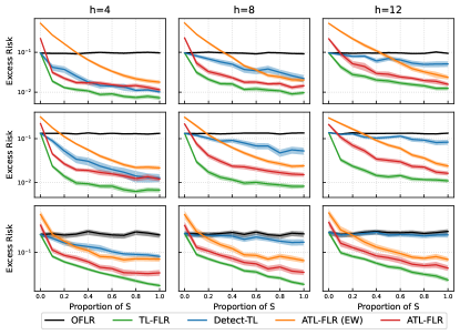
We illustrate our algorithms for FLR by providing results using simulated data and defer the financial market data application and FGLM results to Appendix E. We consider the following, OFLR, TL-FLR, ATL-FLR, Detection Transfer Learning (Detect-TL) [Tian and Feng, 2022] and Exponential Weighted ATL-FLR (ATL-FLR (EW)). To set up the RKHS, we consider the setting in Cai and Yuan [2012]. Let ψk(s)=2cos(πks)\psi_{k}(s)=\sqrt{2}\cos(\pi ks) for j1j\geq 1 and define the reproducing kernel KK of K\mathcal{H}_{K} as K(,)=k=1k2ψk()ψk()K(\cdot,\cdot)=\sum_{k=1}^{\infty}k^{-2}\psi_{k}(\cdot)\psi_{k}(\cdot).

For the target model, β(0)(s)\beta^{(0)}(s) is set to be (1) β1(0)(s)=k=142(1)k1k2ψk(s)\beta_{1}^{(0)}(s)=\sum_{k=1}^{\infty}4\sqrt{2}(-1)^{k-1}k^{-2}\psi_{k}(s); (2) β2(0)(s)=4cos(3πs)\beta_{2}^{(0)}(s)=4\cos(3\pi s); (3) β3(0)(s)=4cos(3πs)+4sin(3πs)\beta_{3}^{(0)}(s)=4\cos(3\pi s)+4\sin(3\pi s). For a specific hh, let 𝒮={l:β0βtKh}\mathcal{S}=\{l:\|\beta_{0}-\beta_{t}\|_{K}\leq h\}, then we generate source models as follows. We scale each target model such that their RKHS norm is 2020. If t𝒮t\in\mathcal{S}, then βt(t)\beta_{t}(t) is set to be βt(s)=β0(s)+k=1(𝒰k(12h/πk2))ψk(s)\beta_{t}(s)=\beta_{0}(s)+\sum_{k=1}^{\infty}\left(\mathcal{U}_{k}(\sqrt{12}h/\pi k^{2})\right)\psi_{k}(s) with 𝒰k\mathcal{U}_{k}’s i.i.d. uniform random variable on [1,1][-1,1]. If t𝒮ct\in\mathcal{S}^{c}, then βt(s)\beta_{t}(s) is generated from a Gaussian process with mean function cos(2πs)\cos(2\pi s) with kernel exp(15|st|)\exp(-15|s-t|) as covariance kernel. The predictors X(t)X^{(t)} are i.i.d. generated from a Gaussian process with the mean function sin(πs)\sin(\pi s) and the covariance kernels are set to be Matérn kernel Cν,ρC_{\nu,\rho} [Cressie and Huang, 1999] where the parameter ν\nu controls the smoothness of X(t)X^{(t)}. We set the covariance kernel of X(t)X^{(t)} as C1/2,1C_{1/2,1} for the target tasks and C3/2,1C_{3/2,1} for source tasks, to fulfill Assumptions 2. We note that such a setting is more challenging than assuming that the target and source tasks have the same covariance kernel. All functions are generated on [0,1][0,1] with 50 evenly spaced points and we set n0=150n_{0}=150 and nt=100n_{t}=100. For each algorithm, we set the regularization parameters as λ1\lambda_{1} and λ2\lambda_{2} as the optimal values in Theorem 1 and select the constants using cross-validation. The excess risk for the target tasks is calculated via the Monte-Carlo method by using 10001000 newly generated predictors X(0)X^{(0)}.

Refer to caption
Figure 2: Left panel (Heatmap): log relative excess risk of TL-FLR to OFLR. Right panels (Line Chart): Excess Risk of different transfer learning algorithms. Each row corresponds to a β(0)\beta^{(0)} and the y-axes for each row are under the same scale. The result for each sample size is an average of 100 replicate experiments with the shaded area indicating ±\pm 2 standard error.

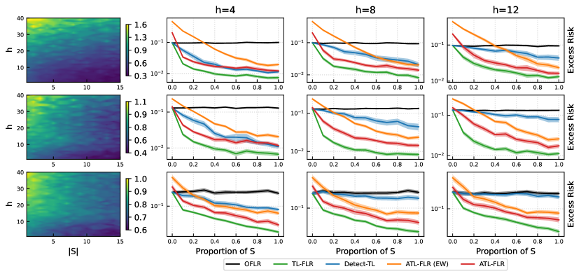
In the left panel of Figure 2 we compare TL-FLR with OFLR by considering relative excess risk, i.e. the ratio of TL-FLR’s excess risk to OFLR’s. We note that since RKHS of β(0)\beta^{(0)} is fixed, the magnitude of hh is proportional to ξ(h,β𝒮)\xi(h,\beta_{\mathcal{S}}) and a large hh indicates less similarity between sources and target tasks. Overall, the effectiveness of TL-FLR for different β(0)\beta^{(0)} presents a consistent pattern, i.e, with more transferable sources involved and smaller hh (bottom right), TL-FLR has a more significant improvement, while with fewer sources and larger hh (top left), the transfer may be worse than OFLR.

In the right panel of Figure 2, we evaluate ATL-FLR under unknown 𝒮\mathcal{S} cases. We set 𝒮\mathcal{S} as a random subset of {1,2,,20}\{1,2,\cdots,20\} such that |𝒮||\mathcal{S}| is equal to 0,2,,200,2,\cdots,20. We also implement TL-FLR by using true 𝒮\mathcal{S} and OFLR as baseline. In all scenarios, ATL-FLR outperforms all its competitors. Comparing ATL-FLR with ATL-FLR(EW), even though ATL-FLR(EW) has similar patterns as ATL-FLR, we can see the gaps between the two curves are larger when the proportion of 𝒮\mathcal{S} is small, showing that ATL-FLR(EW) is more sensitive to source tasks in 𝒮c\mathcal{S}^{c}, while ATL-FLR is less affected. Detect-TL only has a considerable reduction on the excess risk with relatively small hh, but provides limited improvement when hh is large, indicating its limited learning effect when there is only limited knowledge available in sources.

7 Conclusion

In this paper, we study offset transfer learning in functional regression settings including FLR and FGLM. We derive excess risk and show a faster statistical rate depending on both source sample size and the magnitude of similarity across tasks. Our theoretical analysis will help researchers better understand the transfer dynamic of offset transfer learning. Moreover, we leverage the sparse aggregation to alleviate the negative transfer effect while having faster-decreasing aggregation costs compared to transfer learning risk.

References

  • Aghbalou and Staerman [2023] Anass Aghbalou and Guillaume Staerman. Hypothesis transfer learning with surrogate classification losses: Generalization bounds through algorithmic stability. In International Conference on Machine Learning, pages 280–303. PMLR, 2023.
  • Audibert [2009] Jean-Yves Audibert. Fast learning rates in statistical inference through aggregation. The Annals of Statistics, 37(4):1591–1646, 2009.
  • Baker [1973] Charles R Baker. On equivalence of probability measures. The Annals of Probability, pages 690–698, 1973.
  • Balasubramanian et al. [2022] Krishnakumar Balasubramanian, Hans-Georg Müller, and Bharath K Sriperumbudur. Unified rkhs methodology and analysis for functional linear and single-index models. arXiv preprint arXiv:2206.03975, 2022.
  • Bastani [2021] Hamsa Bastani. Predicting with proxies: Transfer learning in high dimension. Management Science, 67(5):2964–2984, 2021.
  • Cai and Wei [2021] T Tony Cai and Hongji Wei. Transfer learning for nonparametric classification: Minimax rate and adaptive classifier. The Annals of Statistics, 49(1):100–128, 2021.
  • Cai and Yuan [2012] T Tony Cai and Ming Yuan. Minimax and adaptive prediction for functional linear regression. Journal of the American Statistical Association, 107(499):1201–1216, 2012.
  • Cardot et al. [1999] Hervé Cardot, Frédéric Ferraty, and Pascal Sarda. Functional linear model. Statistics & Probability Letters, 45(1):11–22, 1999.
  • Cheng and Shang [2015] Guang Cheng and Zuofeng Shang. Joint asymptotics for semi-nonparametric regression models with partially linear structure. The Annals of Statistics, 43(3):1351–1390, 2015.
  • Cressie and Huang [1999] Noel Cressie and Hsin-Cheng Huang. Classes of nonseparable, spatio-temporal stationary covariance functions. Journal of the American Statistical association, 94(448):1330–1339, 1999.
  • Dai et al. [2012] Dong Dai, Philippe Rigollet, and Tong Zhang. Deviation optimal learning using greedy qq-aggregation. The Annals of Statistics, 40(3):1878–1905, 2012.
  • Dalalyan and Tsybakov [2007] Arnak S Dalalyan and Alexandre B Tsybakov. Aggregation by exponential weighting and sharp oracle inequalities. In International Conference on Computational Learning Theory, pages 97–111. Springer, 2007.
  • Du and Wang [2014] Pang Du and Xiao Wang. Penalized likelihood functional regression. Statistica Sinica, pages 1017–1041, 2014.
  • Du et al. [2017] Simon S Du, Jayanth Koushik, Aarti Singh, and Barnabás Póczos. Hypothesis transfer learning via transformation functions. Advances in neural information processing systems, 30, 2017.
  • Du et al. [2020] Simon S Du, Wei Hu, Sham M Kakade, Jason D Lee, and Qi Lei. Few-shot learning via learning the representation, provably. arXiv preprint arXiv:2002.09434, 2020.
  • Gaîffas and Lecué [2011] Stéphane Gaîffas and Guillaume Lecué. Hyper-sparse optimal aggregation. The Journal of Machine Learning Research, 12:1813–1833, 2011.
  • Hall and Horowitz [2007] Peter Hall and Joel L Horowitz. Methodology and convergence rates for functional linear regression. The Annals of Statistics, 35(1):70–91, 2007.
  • Hall and Hosseini-Nasab [2006] Peter Hall and Mohammad Hosseini-Nasab. On properties of functional principal components analysis. Journal of the Royal Statistical Society: Series B (Statistical Methodology), 68(1):109–126, 2006.
  • Juditsky et al. [2008] Anatoli Juditsky, Philippe Rigollet, and Alexandre B Tsybakov. Learning by mirror averaging. The Annals of Statistics, 36(5):2183–2206, 2008.
  • Kokoszka and Reimherr [2017] Piotr Kokoszka and Matthew Reimherr. Introduction to functional data analysis. Chapman and Hall/CRC, 2017.
  • Kuzborskij and Orabona [2013] Ilja Kuzborskij and Francesco Orabona. Stability and hypothesis transfer learning. In International Conference on Machine Learning, pages 942–950. PMLR, 2013.
  • Kuzborskij and Orabona [2017] Ilja Kuzborskij and Francesco Orabona. Fast rates by transferring from auxiliary hypotheses. Machine Learning, 106:171–195, 2017.
  • Leung and Barron [2006] Gilbert Leung and Andrew R Barron. Information theory and mixing least-squares regressions. IEEE Transactions on information theory, 52(8):3396–3410, 2006.
  • Li et al. [2022] Sai Li, T Tony Cai, and Hongzhe Li. Transfer learning for high-dimensional linear regression: Prediction, estimation and minimax optimality. Journal of the Royal Statistical Society Series B: Statistical Methodology, 84(1):149–173, 2022.
  • Li and Bilmes [2007] Xiao Li and Jeff Bilmes. A bayesian divergence prior for classiffier adaptation. In Artificial Intelligence and Statistics, pages 275–282. PMLR, 2007.
  • Orabona et al. [2009] Francesco Orabona, Claudio Castellini, Barbara Caputo, Angelo Emanuele Fiorilla, and Giulio Sandini. Model adaptation with least-squares svm for adaptive hand prosthetics. In 2009 IEEE international conference on robotics and automation, pages 2897–2903. IEEE, 2009.
  • Perrot and Habrard [2015] Michaël Perrot and Amaury Habrard. A theoretical analysis of metric hypothesis transfer learning. In International Conference on Machine Learning, pages 1708–1717. PMLR, 2015.
  • Qu et al. [2016] Simeng Qu, Jane-Ling Wang, and Xiao Wang. Optimal estimation for the functional cox model. The Annals of Statistics, 44(4):1708–1738, 2016.
  • Ramsay et al. [2005] Jim Ramsay, James Ramsay, BW Silverman, et al. Functional Data Analysis. Springer Science & Business Media, 2005.
  • Reimherr et al. [2018] Matthew Reimherr, Bharath Sriperumbudur, and Bahaeddine Taoufik. Optimal prediction for additive function-on-function regression. Electronic Journal of Statistics, 12(2):4571–4601, 2018.
  • Sun et al. [2018] Xiaoxiao Sun, Pang Du, Xiao Wang, and Ping Ma. Optimal penalized function-on-function regression under a reproducing kernel hilbert space framework. Journal of the American Statistical Association, 113(524):1601–1611, 2018.
  • Tian and Feng [2022] Ye Tian and Yang Feng. Transfer learning under high-dimensional generalized linear models. Journal of the American Statistical Association, pages 1–14, 2022.
  • Torrey and Shavlik [2010] Lisa Torrey and Jude Shavlik. Transfer learning. In Handbook of research on machine learning applications and trends: algorithms, methods, and techniques, pages 242–264. IGI global, 2010.
  • Tripuraneni et al. [2020] Nilesh Tripuraneni, Michael Jordan, and Chi Jin. On the theory of transfer learning: The importance of task diversity. Advances in neural information processing systems, 33:7852–7862, 2020.
  • Vaart and Wellner [1996] Aad W Vaart and Jon A Wellner. Weak convergence. In Weak convergence and empirical processes, pages 16–28. Springer, 1996.
  • Varshamov [1957] Rom Rubenovich Varshamov. Estimate of the number of signals in error correcting codes. Docklady Akad. Nauk, SSSR, 117:739–741, 1957.
  • Wang and Schneider [2015] Xuezhi Wang and Jeff G Schneider. Generalization bounds for transfer learning under model shift. In UAI, pages 922–931, 2015.
  • Wang et al. [2016] Xuezhi Wang, Junier B Oliva, Jeff G Schneider, and Barnabás Póczos. Nonparametric risk and stability analysis for multi-task learning problems. In IJCAI, pages 2146–2152, 2016.
  • Wendland [2004] Holger Wendland. Scattered data approximation, volume 17. Cambridge university press, 2004.
  • Xu and Tewari [2021] Ziping Xu and Ambuj Tewari. Representation learning beyond linear prediction functions. Advances in Neural Information Processing Systems, 34:4792–4804, 2021.
  • Yao et al. [2005] Fang Yao, Hans-Georg Müller, and Jane-Ling Wang. Functional linear regression analysis for longitudinal data. The Annals of Statistics, 33(6):2873–2903, 2005.
  • Yuan and Cai [2010] Ming Yuan and T Tony Cai. A reproducing kernel hilbert space approach to functional linear regression. The Annals of Statistics, 38(6):3412–3444, 2010.
  • Zhu et al. [2021] Jiacheng Zhu, Aritra Guha, Mengdi Xu, Yingchen Ma, Rayleigh Lei, Vincenzo Loffredo, XuanLong Nguyen, and Ding Zhao. Functional optimal transport: Mapping estimation and domain adaptation for functional data. 2021.

Appendix A Appendix: Background of RKHS and Integral Operators

In this section, we will present some facts about the RKHS and also the integral operator of a kernel that are useful in our proof and refer readers to Wendland [2004] for a more detailed discussion.

Let 𝒯\mathcal{T} be a compact set of \mathbb{R}. For a real, symmetric, square-integrable, and semi-positive definite kernel K:𝒯×𝒯K:\mathcal{T}\times\mathcal{T}\rightarrow\mathbb{R}, we denote its associated RKHS as K\mathcal{H}_{K}. For the reproducing kernel KK, we can define its integral operator LK:L2L2L_{K}:L^{2}\rightarrow L^{2} as

LK(f)()=𝒯K(s,)f(s)𝑑s.L_{K}(f)(\cdot)=\int_{\mathcal{T}}K(s,\cdot)f(s)ds.

LKL_{K} is self-adjoint, positive-definite, and trace class (thus Hilbert-Schmidt and compact). By the spectral theorem for self-adjoint compact operators, there exists an at most countable index set NN, a non-increasing summable positive sequence {τj}j1\{\tau_{j}\}_{j\geq 1} and an orthonormal basis of L2L^{2}, {ej}j1\{e_{j}\}_{j\geq 1} such that the integrable operator can be expressed as

LK()=jNτj,ejL2ej.L_{K}(\cdot)=\sum_{j\in N}\tau_{j}\langle\cdot,e_{j}\rangle_{L^{2}}e_{j}.

The sequence {τj}j1\{\tau_{j}\}_{j\geq 1} and the basis {ej}j1\{e_{j}\}_{j\geq 1} are referred as the eigenvalues and eigenfunctions. The Mercer’s theorem shows that the kernel KK itself can be expressed as

K(x,x)=jNτjej(x)ej(x),x,x𝒯,K(x,x^{\prime})=\sum_{j\in N}\tau_{j}e_{j}(x)e_{j}(x^{\prime}),\quad\forall x,x^{\prime}\in\mathcal{T},

where the convergence is absolute and uniform.

We now introduce the fractional power integral operator and the composite integral operator of two kernels. For any s0s\geq 0, the fractional power integral operator LKs:L2L2L_{K}^{s}:L^{2}\rightarrow L^{2} is defined as

LKs()=jNτjs,ejL2ej.L_{K}^{s}(\cdot)=\sum_{j\in N}\tau_{j}^{s}\langle\cdot,e_{j}\rangle_{L^{2}}e_{j}.

For two kernels K1K_{1} and K2K_{2}, we define their composite kernel as

(K1K2)(x,x)=𝒯K1(x,s)K2(s,x)𝑑s,(K_{1}K_{2})(x,x^{\prime})=\int_{\mathcal{T}}K_{1}(x,s)K_{2}(s,x^{\prime})ds,

and thus LK2K2=LK1LK2L_{K_{2}K_{2}}=L_{K_{1}}\circ L_{K_{2}}. Given these definitions, for a given reproducing kernel KK and covariance function CC, the definition of Γ\Gamma in the main paper is

LΓ=LK12LCLK12andΓ:=K12CK12.L_{\Gamma}=L_{K^{\frac{1}{2}}}\circ L_{C}\circ L_{K^{\frac{1}{2}}}\quad\text{and}\quad\Gamma:=K^{\frac{1}{2}}CK^{\frac{1}{2}}.

If both LK12L_{K^{\frac{1}{2}}} and LCL_{C} are bounded linear operators, the spectral algorithm guarantees the existence of eigenvalues {sj}j1\{s_{j}\}_{j\geq 1} and eigenfunctions {ψj}j1\{\psi_{j}\}_{j\geq 1}.

Appendix B Appendix: Sparse Aggregation Process

We provide the procedure of sparse aggregation in Step 4 of ATL-FLR (Algorithm 2) for readers’ reference and refer readers to Gaîffas and Lecué [2011] for more detail.

The sparse aggregation algorithm is stated in Algorithm 3. For the Oracle inequality and the pre-specified parameter cc and ϕ\phi, we refer the reader to Appendix C.5 for model detail. In general, the final aggregated estimator β^a\hat{\beta}_{a} will only select two of the best-performed candidates from the candidates set \mathcal{F}. This guarantees some of the incorrectly constructed 𝒮^\hat{\mathcal{S}} are not involved in building β^a\hat{\beta}_{a} and thus alleviate the negative transfer sources.

Algorithm 3 Sparse Aggregation
1:Input: The candidate set \mathcal{F}; target dataset 𝒟c(0)\mathcal{D}_{\mathcal{I}^{c}}^{(0)}; pre-specified parameter cc, ϕ\phi.
2:
3:Split 𝒟c(0)\mathcal{D}_{\mathcal{I}^{c}}^{(0)} into equal size set, with index set 1c\mathcal{I}_{1}^{c} and 2c\mathcal{I}_{2}^{c}
4:Use 𝒟1c(0)\mathcal{D}_{\mathcal{I}_{1}^{c}}^{(0)} to define a random subset of \mathcal{F} as
1={β:Rn,1c(β)Rn,1c(β^n1)+cmax(ϕβ^n1βn,1c,ϕ2)}\mathcal{F}_{1}=\left\{\beta\in\mathcal{F}:R_{n,\mathcal{I}_{1}^{c}}(\beta)\leq R_{n,\mathcal{I}_{1}^{c}}(\hat{\beta}_{n1})+c\max\left(\phi\left\|\hat{\beta}_{n1}-\beta\right\|_{n,\mathcal{I}_{1}^{c}},\phi^{2}\right)\right\}
where
βn,1c2=1|1c|i1cXi(0),βL22,Rn,(β)=1||i(Yi(0)Xi(0),βL2)2,β^n1=argminβRn,1c(β)\left\|\beta\right\|_{n,\mathcal{I}_{1}^{c}}^{2}=\frac{1}{|\mathcal{I}_{1}^{c}|}\sum_{i\in\mathcal{I}_{1}^{c}}\langle X_{i}^{(0)},\beta\rangle_{L^{2}}^{2},\quad R_{n,\mathcal{I}}(\beta)=\frac{1}{|\mathcal{I}|}\sum_{i\in\mathcal{I}}(Y_{i}^{(0)}-\langle X_{i}^{(0)},\beta\rangle_{L^{2}})^{2},\quad\hat{\beta}_{n1}=\underset{\beta\in\mathcal{F}}{argmin}R_{n,\mathcal{I}_{1}^{c}}(\beta)
5:Set 2\mathcal{F}_{2} as following:
2={c1β1+c2β2:β1,β21andc1+c2=1}\mathcal{F}_{2}=\{c_{1}\beta_{1}+c_{2}\beta_{2}:\beta_{1},\beta_{2}\in\mathcal{F}_{1}\ \textit{and}\ c_{1}+c_{2}=1\}
then, return
β^a=argminβ2Rn,2c(β).\hat{\beta}_{a}=\underset{\beta\in\mathcal{F}_{2}}{argmin}R_{n,\mathcal{I}_{2}^{c}}(\beta).
Remark 5.

In Gaîffas and Lecué [2011], the authors indicated β^a\hat{\beta}_{a} has a explicit solution with the form

β^a=t^β^1+(1t^)β^2\hat{\beta}_{a}=\hat{t}\hat{\beta}_{1}+(1-\hat{t})\hat{\beta}_{2}

with β^1\hat{\beta}_{1} and β^2\hat{\beta}_{2} in belongs to \mathcal{F} and t^\hat{t} has an analytical form.

Appendix C Appendix: Proof of Section 4

C.1 Proof of Upper Bound for TL-FLR (Theorem 1)

Proof.

We first prove the upper bound under Assumption 2 condition 1 and defer the proof under condition 2 at the end. WLOG, we assume the eigenfunction of LΓ(0)L_{\Gamma^{(0)}} and LΓ(t)L_{\Gamma^{(t)}} are perfectly aligned, i.e. ϕj(0)=ϕj(t)\phi_{j}^{(0)}=\phi_{j}^{(t)} for all jj\in\mathbb{N}. We also We also recall that we set all the intercept α(t)=0\alpha^{(t)}=0 since α(t)\alpha^{(t)} will not affect the convergence rate of estimating β(t)\beta^{(t)} [Du and Wang, 2014].

Let L2={f:𝒯:fL2<}L^{2}=\{f:\mathcal{T}\rightarrow\mathbb{R}:\|f\|_{L^{2}}<\infty\} represent the he set of all square integrable functions over 𝒯\mathcal{T}. Since LK12(L2)=KL_{K^{\frac{1}{2}}}(L^{2})=\mathcal{H}_{K}, for any βK\beta\in\mathcal{H}_{K}, there exist a fL2f\in L^{2} such that β=LK12(f)\beta=L_{K^{\frac{1}{2}}}(f). In following proofs, we denote f(t)f^{(t)} as β(t)\beta^{(t)}’s corresponding element in L2L^{2}. Therefore, we can rewrite the minimization problem in the transfer step and the calibrate step as

f^𝒮λ1=argminfL2{1n𝒮t𝒮i=1nt(Yi(t)Xi(t),LK12(f))2+λ1fL22},\hat{f}_{\mathcal{S}\lambda_{1}}=\underset{f\in L^{2}}{\operatorname{argmin}}\left\{\frac{1}{n_{\mathcal{S}}}\sum_{t\in\mathcal{S}}\sum_{i=1}^{n_{t}}\left(Y_{i}^{(t)}-\langle X_{i}^{(t)},L_{K^{\frac{1}{2}}}(f)\rangle\right)^{2}+\lambda_{1}\|f\|_{L^{2}}^{2}\right\},

where n𝒮=t𝒮ntn_{\mathcal{S}}=\sum_{t\in\mathcal{S}}n_{t} and

f^δλ2=argminfδL2{1n0i=1n0(Yi(0)Xi(0),LK12(f^𝒮+fδ))2+λ2fδL22}.\hat{f}_{\delta\lambda_{2}}=\underset{f_{\delta}\in L^{2}}{\operatorname{argmin}}\left\{\frac{1}{n_{0}}\sum_{i=1}^{n_{0}}\left(Y_{i}^{(0)}-\langle X_{i}^{(0)},L_{K^{\frac{1}{2}}}(\hat{f}_{\mathcal{S}}+f_{\delta})\rangle\right)^{2}+\lambda_{2}\|f_{\delta}\|_{L^{2}}^{2}\right\}.

Thus the excess risk of β^\hat{\beta} can be rewritten as

(β^)=(LΓ(0))12(f^f0)L22wheref^=f^𝒮λ1+f^δλ1\mathcal{E}(\hat{\beta})=\left\|(L_{\Gamma^{(0)}})^{\frac{1}{2}}(\hat{f}-f_{0})\right\|_{L^{2}}^{2}\quad\text{where}\quad\hat{f}=\hat{f}_{\mathcal{S}\lambda_{1}}+\hat{f}_{\delta\lambda_{1}}

Define the empirical version of C(t)C^{(t)} as

Cn(t)(s,t)=1nti=1ntXi(t)(s)Xi(t)(t),C_{n}^{(t)}(s,t)=\frac{1}{n_{t}}\sum_{i=1}^{n_{t}}X_{i}^{(t)}(s)X_{i}^{(t)}(t),

and let

LΓn(t)=LK12LCn(t)LK12.L_{\Gamma_{n}^{(t)}}=L_{K^{\frac{1}{2}}}L_{C_{n}^{(t)}}L_{K^{\frac{1}{2}}}.

To bound the excess risk (β^)\mathcal{E}(\hat{\beta}), by triangle inequality,

(LΓ(0))12(f^f0)L2(LΓ(0))12(f^𝒮f𝒮)L2+(LΓ(0))12(f^δfδ)L2\left\|(L_{\Gamma^{(0)}})^{\frac{1}{2}}(\hat{f}-f_{0})\right\|_{L^{2}}\leq\left\|(L_{\Gamma^{(0)}})^{\frac{1}{2}}(\hat{f}_{\mathcal{S}}-f_{\mathcal{S}})\right\|_{L^{2}}+\left\|(L_{\Gamma^{(0)}})^{\frac{1}{2}}(\hat{f}_{\delta}-f_{\delta})\right\|_{L^{2}}

where each term at the r.h.s. corresponds to the excess risk from the transfer and calibrate steps respectively.

Transfer Step.

For the transfer step, the solution of minimization is

f^𝒮λ1=(t𝒮αtLΓn(t)+λ1𝐈)1(t𝒮αtLΓn(t)(f(t))+t𝒮gn(t)),\hat{f}_{\mathcal{S}\lambda_{1}}=\left(\sum_{t\in\mathcal{S}}\alpha_{t}L_{\Gamma_{n}^{(t)}}+\lambda_{1}\mathbf{I}\right)^{-1}\left(\sum_{t\in\mathcal{S}}\alpha_{t}L_{\Gamma_{n}^{(t)}}(f^{(t)})+\sum_{t\in\mathcal{S}}g_{n}^{(t)}\right),

where 𝐈\mathbf{I} is identity operator, αt=ntn𝒮\alpha_{t}=\frac{n_{t}}{n_{\mathcal{S}}} and

gn(t)=1n𝒮i=1ntϵi(t)LK12(Xi(t)).g_{n}^{(t)}=\frac{1}{n_{\mathcal{S}}}\sum_{i=1}^{n_{t}}\epsilon_{i}^{(t)}L_{K^{\frac{1}{2}}}(X_{i}^{(t)}).

Besides, the solution of the transfer learning step, f^𝒮λ1\hat{f}_{\mathcal{S}\lambda_{1}}, converges to its population version, which is defined by the following moment condition

t𝒮αtE{LK12(X(t))(Y(t)LK12(X(t)),f𝒮L2)}=0,\sum_{t\in\mathcal{S}}\alpha_{t}\operatorname{E}\left\{L_{K^{\frac{1}{2}}}(X^{(t)})\left(Y^{(t)}-\langle L_{K^{\frac{1}{2}}}(X^{(t)}),f_{\mathcal{S}}\rangle_{L^{2}}\right)\right\}=0,

and therefore leads to the explicit form of f𝒮f_{\mathcal{S}} as

(t𝒮αtLΓ(t))f𝒮=t𝒮αtLΓ(t)(f(t)).\left(\sum_{t\in\mathcal{S}}\alpha_{t}L_{\Gamma^{(t)}}\right)f_{\mathcal{S}}=\sum_{t\in\mathcal{S}}\alpha_{t}L_{\Gamma^{(t)}}\left(f^{(t)}\right).

Define

f𝒮λ1=(t𝒮αtLΓ(t)+λ1𝐈)1(t𝒮αtLΓ(t)(f(t))).f_{\mathcal{S}\lambda_{1}}=\left(\sum_{t\in\mathcal{S}}\alpha_{t}L_{\Gamma^{(t)}}+\lambda_{1}\mathbf{I}\right)^{-1}\left(\sum_{t\in\mathcal{S}}\alpha_{t}L_{\Gamma^{(t)}}(f^{(t)})\right).

By triangle inequality

(LΓ(0))12(f^𝒮λ1f𝒮)L2(LΓ(0))12(f^𝒮λ1f𝒮λ1)L2estimation error+(LΓ(0))12(f𝒮λ1f𝒮)L2approximation error.\left\|(L_{\Gamma^{(0)}})^{\frac{1}{2}}(\hat{f}_{\mathcal{S}\lambda_{1}}-f_{\mathcal{S}})\right\|_{L^{2}}\leq\underbrace{\left\|(L_{\Gamma^{(0)}})^{\frac{1}{2}}(\hat{f}_{\mathcal{S}\lambda_{1}}-f_{\mathcal{S}\lambda_{1}})\right\|_{L^{2}}}_{\text{estimation error}}+\underbrace{\left\|(L_{\Gamma^{(0)}})^{\frac{1}{2}}(f_{\mathcal{S}\lambda_{1}}-f_{\mathcal{S}})\right\|_{L^{2}}}_{\text{approximation error}}.

For approximation error, by Lemma 1 and taking v=12v=\frac{1}{2}, the second term on r.h.s. can be bounded by

(LΓ(0))12(f𝒮λ1f𝒮)L22=O(λ1f𝒮L22).\left\|(L_{\Gamma^{(0)}})^{\frac{1}{2}}(f_{\mathcal{S}\lambda_{1}}-f_{\mathcal{S}})\right\|_{L^{2}}^{2}=O_{\mathbb{P}}\left(\lambda_{1}\left\|f_{\mathcal{S}}\right\|_{L^{2}}^{2}\right).

Now we turn to the estimation error. We further introduce an intermedia term

f~𝒮λ1=f𝒮λ1+(t𝒮αtLΓ(t)+λ1𝐈)1(t𝒮αtLΓn(t)(f𝒮f𝒮λ1)+t𝒮gn(t)λ1f𝒮λ1).\tilde{f}_{\mathcal{S}\lambda_{1}}=f_{\mathcal{S}\lambda_{1}}+\left(\sum_{t\in\mathcal{S}}\alpha_{t}L_{\Gamma^{(t)}}+\lambda_{1}\mathbf{I}\right)^{-1}\left(\sum_{t\in\mathcal{S}}\alpha_{t}L_{\Gamma_{n}^{(t)}}(f_{\mathcal{S}}-f_{\mathcal{S}\lambda_{1}})+\sum_{t\in\mathcal{S}}g_{n}^{(t)}-\lambda_{1}f_{\mathcal{S}\lambda_{1}}\right).

We first bound (LΓ(0))12(f𝒮λ1f~𝒮λ1)L22\|(L_{\Gamma^{(0)}})^{\frac{1}{2}}(f_{\mathcal{S}\lambda_{1}}-\tilde{f}_{\mathcal{S}\lambda_{1}})\|_{L^{2}}^{2}. Based on he fact that

λ1f𝒮λ1=t𝒮αtLΓ(t)(f(t)f𝒮λ1)=t𝒮αtLΓ(t)(f𝒮f𝒮λ1),\lambda_{1}f_{\mathcal{S}\lambda_{1}}=\sum_{t\in\mathcal{S}}\alpha_{t}L_{\Gamma^{(t)}}\left(f^{(t)}-f_{\mathcal{S}\lambda_{1}}\right)=\sum_{t\in\mathcal{S}}\alpha_{t}L_{\Gamma^{(t)}}\left(f_{\mathcal{S}}-f_{\mathcal{S}\lambda_{1}}\right),

we have

(LΓ(0))12(f𝒮λ1f~𝒮λ1)L2\displaystyle\|(L_{\Gamma^{(0)}})^{\frac{1}{2}}(f_{\mathcal{S}\lambda_{1}}-\tilde{f}_{\mathcal{S}\lambda_{1}})\|_{L^{2}}
(LΓ(0))12(t𝒮αtLΓ(t)+λ1𝐈)1(t𝒮gn(t))L2+\displaystyle\quad\leq\left\|(L_{\Gamma^{(0)}})^{\frac{1}{2}}(\sum_{t\in\mathcal{S}}\alpha_{t}L_{\Gamma^{(t)}}+\lambda_{1}\mathbf{I})^{-1}(\sum_{t\in\mathcal{S}}g_{n}^{(t)})\right\|_{L^{2}}+
(LΓ(0))12(t𝒮αtLΓ(t)+λ1𝐈)1(t𝒮αt(LΓn(t)LΓ(t))(f𝒮f𝒮λ1))L2\displaystyle\quad\qquad\left\|(L_{\Gamma^{(0)}})^{\frac{1}{2}}(\sum_{t\in\mathcal{S}}\alpha_{t}L_{\Gamma^{(t)}}+\lambda_{1}\mathbf{I})^{-1}(\sum_{t\in\mathcal{S}}\alpha_{t}(L_{\Gamma_{n}^{(t)}}-L_{\Gamma^{(t)}})(f_{\mathcal{S}}-f_{\mathcal{S}\lambda_{1}}))\right\|_{L^{2}}
={j=1((LΓ(0))12(t𝒮αtLΓ(t)+λ1𝐈)1(t𝒮gn(t)),ϕj(0))L2)2}12+\displaystyle\quad=\left\{\sum_{j=1}^{\infty}\left(\left\langle(L_{\Gamma^{(0)}})^{\frac{1}{2}}(\sum_{t\in\mathcal{S}}\alpha_{t}L_{\Gamma^{(t)}}+\lambda_{1}\mathbf{I})^{-1}\left(\sum_{t\in\mathcal{S}}g_{n}^{(t)}\right),\phi_{j}^{(0)})\right\rangle_{L^{2}}\right)^{2}\right\}^{\frac{1}{2}}+
{j=1((LΓ(0))12(t𝒮αtLΓ(t)+λ1𝐈)1(t𝒮αt(LΓn(t)LΓ(t))(f𝒮f𝒮λ1)),ϕj(0))L2)2}12\displaystyle\quad\qquad\left\{\sum_{j=1}^{\infty}\left(\left\langle(L_{\Gamma^{(0)}})^{\frac{1}{2}}(\sum_{t\in\mathcal{S}}\alpha_{t}L_{\Gamma^{(t)}}+\lambda_{1}\mathbf{I})^{-1}\left(\sum_{t\in\mathcal{S}}\alpha_{t}(L_{\Gamma_{n}^{(t)}}-L_{\Gamma^{(t)}})(f_{\mathcal{S}}-f_{\mathcal{S}\lambda_{1}})\right),\phi_{j}^{(0)})\right\rangle_{L^{2}}\right)^{2}\right\}^{\frac{1}{2}}

For the first term in the above inequality, by Lemma 3,

{j=1((LΓ(0))12(t𝒮αtLΓ(t)+λ1𝐈)1(t𝒮gn(t)),ϕj(0))L2)2}=O(σ2(n𝒮)1λ112r).\left\{\sum_{j=1}^{\infty}\left(\left\langle(L_{\Gamma^{(0)}})^{\frac{1}{2}}(\sum_{t\in\mathcal{S}}\alpha_{t}L_{\Gamma^{(t)}}+\lambda_{1}\mathbf{I})^{-1}\left(\sum_{t\in\mathcal{S}}g_{n}^{(t)}\right),\phi_{j}^{(0)})\right\rangle_{L^{2}}\right)^{2}\right\}=O_{\mathbb{P}}\left(\sigma^{2}\left(n_{\mathcal{S}}\right)^{-1}\lambda_{1}^{\frac{1}{2r}}\right).

For second one, by Lemma 2 and 4,

j=1((LΓ(0))12(t𝒮αtLΓ(t)+λ1𝐈)1(t𝒮αt(LΓn(t)LΓ(t))(f𝒮f𝒮λ1)),ϕj(0))L2)2=O((n𝒮)1λ112r).\sum_{j=1}^{\infty}\left(\left\langle(L_{\Gamma^{(0)}})^{\frac{1}{2}}(\sum_{t\in\mathcal{S}}\alpha_{t}L_{\Gamma^{(t)}}+\lambda_{1}\mathbf{I})^{-1}\left(\sum_{t\in\mathcal{S}}\alpha_{t}(L_{\Gamma_{n}^{(t)}}-L_{\Gamma^{(t)}})(f_{\mathcal{S}}-f_{\mathcal{S}\lambda_{1}})\right),\phi_{j}^{(0)})\right\rangle_{L^{2}}\right)^{2}=O_{\mathbb{P}}\left(\left(n_{\mathcal{S}}\right)^{-1}\lambda_{1}^{\frac{1}{2r}}\right).

Therefore,

(LΓ(0))12(f𝒮λ1f~𝒮λ1)L22=O(f𝒮L22(n𝒮)1λ112r).\|(L_{\Gamma^{(0)}})^{\frac{1}{2}}(f_{\mathcal{S}\lambda_{1}}-\tilde{f}_{\mathcal{S}\lambda_{1}})\|_{L^{2}}^{2}=O_{\mathbb{P}}\left(\|f_{\mathcal{S}}\|_{L^{2}}^{2}\left(n_{\mathcal{S}}\right)^{-1}\lambda_{1}^{\frac{1}{2r}}\right).

Finally, we bound (LΓ(0))12(f^𝒮λ1f~𝒮λ1)L22\|(L_{\Gamma^{(0)}})^{\frac{1}{2}}(\hat{f}_{\mathcal{S}\lambda_{1}}-\tilde{f}_{\mathcal{S}\lambda_{1}})\|_{L^{2}}^{2}. Once again, by the definition of f~𝒮λ1\tilde{f}_{\mathcal{S}\lambda_{1}}

f^𝒮λ1f~𝒮λ1=(t𝒮αtLΓ(t)+λ1𝐈)1(t𝒮αt(LΓ(t)LΓn(t))(f^𝒮λ1f𝒮λ1)).\hat{f}_{\mathcal{S}\lambda_{1}}-\tilde{f}_{\mathcal{S}\lambda_{1}}=\left(\sum_{t\in\mathcal{S}}\alpha_{t}L_{\Gamma^{(t)}}+\lambda_{1}\mathbf{I}\right)^{-1}\left(\sum_{t\in\mathcal{S}}\alpha_{t}(L_{\Gamma^{(t)}}-L_{\Gamma_{n}^{(t)}})(\hat{f}_{\mathcal{S}\lambda_{1}}-f_{\mathcal{S}\lambda_{1}})\right).

Thus, by Lemma 2

(LΓ(0))12(f^𝒮λ1f~𝒮λ1)L22\displaystyle\left\|(L_{\Gamma^{(0)}})^{\frac{1}{2}}(\hat{f}_{\mathcal{S}\lambda_{1}}-\tilde{f}_{\mathcal{S}\lambda_{1}})\right\|_{L^{2}}^{2}
(LΓ(0))12(t𝒮αtLΓ(t)+λ1𝐈)1(t𝒮αt(LΓ(t)LΓn(t)))(LΓ(0))12op2(LΓ(0))12(f^𝒮λ1f𝒮λ1)L22\displaystyle\qquad\leq\left\|(L_{\Gamma^{(0)}})^{\frac{1}{2}}(\sum_{t\in\mathcal{S}}\alpha_{t}L_{\Gamma^{(t)}}+\lambda_{1}\mathbf{I})^{-1}(\sum_{t\in\mathcal{S}}\alpha_{t}\left(L_{\Gamma^{(t)}}-L_{\Gamma_{n}^{(t)}}\right))(L_{\Gamma^{(0)}})^{-\frac{1}{2}}\right\|_{op}^{2}\left\|(L_{\Gamma^{(0)}})^{\frac{1}{2}}(\hat{f}_{\mathcal{S}\lambda_{1}}-f_{\mathcal{S}\lambda_{1}})\right\|_{L^{2}}^{2}
=O(n𝒮1λ112r(LΓ(0))12(f^𝒮λ1f𝒮λ1)L22)\displaystyle\qquad=O_{\mathbb{P}}\left(n_{\mathcal{S}}^{-1}\lambda_{1}^{\frac{1}{2r}}\left\|(L_{\Gamma^{(0)}})^{\frac{1}{2}}(\hat{f}_{\mathcal{S}\lambda_{1}}-f_{\mathcal{S}\lambda_{1}})\right\|_{L^{2}}^{2}\right)
=o((LΓ(0))12(f^𝒮λ1f𝒮λ1)L22).\displaystyle\qquad=o_{\mathbb{P}}\left(\left\|(L_{\Gamma^{(0)}})^{\frac{1}{2}}(\hat{f}_{\mathcal{S}\lambda_{1}}-f_{\mathcal{S}\lambda_{1}})\right\|_{L^{2}}^{2}\right).

Combine three parts, we get

(LΓ(0))12(f^𝒮λ1f𝒮)L22=O(f𝒮L22λ1+(σ2+f𝒮L22)n𝒮1λ112r),\left\|(L_{\Gamma^{(0)}})^{\frac{1}{2}}\left(\hat{f}_{\mathcal{S}\lambda_{1}}-f_{\mathcal{S}}\right)\right\|_{L^{2}}^{2}=O_{\mathbb{P}}\left(\|f_{\mathcal{S}}\|_{L^{2}}^{2}\lambda_{1}+\left(\sigma^{2}+\|f_{\mathcal{S}}\|_{L^{2}}^{2}\right)n_{\mathcal{S}}^{-1}\lambda_{1}^{-\frac{1}{2r}}\right),

by taking λ1(n𝒮)2r2r+1\lambda_{1}\asymp(n_{\mathcal{S}})^{-\frac{2r}{2r+1}} and notice the fact that σ2β𝒮K2\frac{\sigma^{2}}{\|\beta_{\mathcal{S}}\|_{K}^{2}} is bounded above (This is a reasonable condition since the signal-to-noise ratio can’t be 0, otherwise one can hardly learn anything from the data), we have

(LΓ(0))12(f^𝒮λ1f𝒮)L22=O(f𝒮L22n𝒮2r2r+1).\left\|(L_{\Gamma^{(0)}})^{\frac{1}{2}}\left(\hat{f}_{\mathcal{S}\lambda_{1}}-f_{\mathcal{S}}\right)\right\|_{L^{2}}^{2}=O_{\mathbb{P}}\left(\|f_{\mathcal{S}}\|_{L^{2}}^{2}n_{\mathcal{S}}^{-\frac{2r}{2r+1}}\right).

The desired upper bound is proved given the fact that σ2β𝒮K2\frac{\sigma^{2}}{\|\beta_{\mathcal{S}}\|_{K}^{2}} and σ2h2\frac{\sigma^{2}}{h^{2}} is bounded above.

Calibrate Step.

The estimation scheme in the calibrate step is in the same form as the transfer step and thus its proof follows the same logic as the transfer step. The solution to the minimization problem in the calibration step is

f^δλ2=(LΓn(0)+λ2𝐈)1(LΓn(0)(f𝒮f^𝒮λ1+fδ)+gn(0)),\hat{f}_{\delta\lambda_{2}}=\left(L_{\Gamma_{n}^{(0)}}+\lambda_{2}\mathbf{I}\right)^{-1}\left(L_{\Gamma_{n}^{(0)}}(f_{\mathcal{S}}-\hat{f}_{\mathcal{S}\lambda_{1}}+f_{\delta})+g_{n}^{(0)}\right),

where

gn(0)=1n0i=1n0ϵi(0)LK12(Xi(0)).g_{n}^{(0)}=\frac{1}{n_{0}}\sum_{i=1}^{n_{0}}\epsilon_{i}^{(0)}L_{K^{\frac{1}{2}}}(X_{i}^{(0)}).

Similarly, define

fδλ2=(LΓ(0)+λ2𝐈)1(LT(0)(f𝒮f^𝒮+fδ)),f_{\delta\lambda_{2}}=\left(L_{\Gamma^{(0)}}+\lambda_{2}\mathbf{I}\right)^{-1}\left(L_{T^{(0)}}(f_{\mathcal{S}}-\hat{f}_{\mathcal{S}}+f_{\delta})\right),

where fδf_{\delta} is the population version of the estimator, i.e. f^δ\hat{f}_{\delta}.

(t𝒮αtLΓ(t))fδ=(t𝒮αtLΓ(t)(fδ(t)))\left(\sum_{t\in\mathcal{S}}\alpha_{t}L_{\Gamma^{(t)}}\right)f_{\delta}=\left(\sum_{t\in\mathcal{S}}\alpha_{t}L_{\Gamma^{(t)}}\left(f_{\delta}^{(t)}\right)\right)

By triangle inequality,

(LΓ(0))12(f^δfδ)L2(LΓ(0))12(f^δfδλ2)L2+(LΓ(0))12(fδλ2fδ)L2.\left\|(L_{\Gamma^{(0)}})^{\frac{1}{2}}(\hat{f}_{\delta}-f_{\delta})\right\|_{L^{2}}\leq\left\|(L_{\Gamma^{(0)}})^{\frac{1}{2}}(\hat{f}_{\delta}-f_{\delta\lambda_{2}})\right\|_{L^{2}}+\left\|(L_{\Gamma^{(0)}})^{\frac{1}{2}}(f_{\delta\lambda_{2}}-f_{\delta})\right\|_{L^{2}}.

For the second term in r.h.s.,

(LΓ(0))12(fδλ2fδ)L2\displaystyle\left\|(L_{\Gamma^{(0)}})^{\frac{1}{2}}(f_{\delta\lambda_{2}}-f_{\delta})\right\|_{L^{2}} (LΓ(0))12(LΓ(0)+λ2𝐈)1LΓ(0)(f𝒮f^𝒮λ1)L2+(LΓ(0))12(fδλ2fδ)L2\displaystyle\leq\left\|(L_{\Gamma^{(0)}})^{\frac{1}{2}}\left(L_{\Gamma^{(0)}}+\lambda_{2}\mathbf{I}\right)^{-1}L_{\Gamma^{(0)}}\left(f_{\mathcal{S}}-\hat{f}_{\mathcal{S}\lambda_{1}}\right)\right\|_{L^{2}}+\left\|(L_{\Gamma^{(0)}})^{\frac{1}{2}}\left(f_{\delta\lambda_{2}}^{*}-f_{\delta}\right)\right\|_{L^{2}}
(LΓ(0))12(LΓ(0)+λ2𝐈)1(LΓ(0))12opLΓ(0)12(f𝒮f^𝒮)L2\displaystyle\leq\left\|(L_{\Gamma^{(0)}})^{\frac{1}{2}}\left(L_{\Gamma^{(0)}}+\lambda_{2}\mathbf{I}\right)^{-1}(L_{\Gamma^{(0)}})^{\frac{1}{2}}\right\|_{op}\left\|L_{\Gamma^{(0)}}^{\frac{1}{2}}\left(f_{\mathcal{S}}-\hat{f}_{\mathcal{S}}\right)\right\|_{L^{2}}
+(LΓ(0))12(fδλ2fδ)L2,\displaystyle\qquad+\left\|(L_{\Gamma^{(0)}})^{\frac{1}{2}}\left(f_{\delta\lambda_{2}}^{*}-f_{\delta}\right)\right\|_{L^{2}},

where fδλ2=(LΓ(0)+λ2𝐈)1LΓ(0)(fδ)f_{\delta\lambda_{2}}^{*}=\left(L_{\Gamma^{(0)}}+\lambda_{2}\mathbf{I}\right)^{-1}L_{\Gamma^{(0)}}(f_{\delta}).

By Lemma 1 with 𝒮=\mathcal{S}=\emptyset,

(LΓ(0))12(fδλ2fδ)L22\displaystyle\left\|(L_{\Gamma^{(0)}})^{\frac{1}{2}}\left(f_{\delta\lambda_{2}}^{*}-f_{\delta}\right)\right\|_{L^{2}}^{2} λ24fδL22\displaystyle\leq\frac{\lambda_{2}}{4}\left\|f_{\delta}\right\|_{L^{2}}^{2}
λ2h2,\displaystyle\lesssim\lambda_{2}h^{2},

where the second inequality holds with the fact the 𝒮={1lL:f0f(t)L2h}\mathcal{S}=\left\{1\leq l\leq L:\|f_{0}-f^{(t)}\|_{L^{2}}\leq h\right\}. Therefore,

(LΓ(0))12(fδλ2fδ)L22=O(n𝒮2r2r+1+λ2h2).\left\|(L_{\Gamma^{(0)}})^{\frac{1}{2}}(f_{\delta\lambda_{2}}-f_{\delta})\right\|_{L^{2}}^{2}=O_{\mathbb{P}}\left(n_{\mathcal{S}}^{-\frac{2r}{2r+1}}+\lambda_{2}h^{2}\right).

For the first term, we play the same game as transfer step. Define

f~δλ2=fδλ2+(LΓ(0)+λ2𝐈)1(LΓn(0)(f𝒮λ1f^𝒮λ1+fδ)+gn(0)LΓn(0)(fδλ2)λ1fδλ2),\tilde{f}_{\delta\lambda_{2}}=f_{\delta\lambda_{2}}+\left(L_{\Gamma^{(0)}}+\lambda_{2}\mathbf{I}\right)^{-1}\left(L_{\Gamma_{n}^{(0)}}(f_{\mathcal{S}\lambda_{1}}-\hat{f}_{\mathcal{S}\lambda_{1}}+f_{\delta})+g_{n}^{(0)}-L_{\Gamma_{n}^{(0)}}(f_{\delta\lambda_{2}})-\lambda_{1}f_{\delta\lambda_{2}}\right),

and the definition of fδλ2f_{\delta\lambda_{2}} leads to

f~δλ2fδλ2=(LΓ(0)+λ2𝐈)1((LΓn(0)LΓ(0))(f𝒮λ1f^𝒮λ1+fδfδλ2+gn(0))).\tilde{f}_{\delta\lambda_{2}}-f_{\delta\lambda_{2}}=\left(L_{\Gamma^{(0)}}+\lambda_{2}\mathbf{I}\right)^{-1}\left((L_{\Gamma_{n}^{(0)}}-L_{\Gamma^{(0)}})(f_{\mathcal{S}\lambda_{1}}-\hat{f}_{\mathcal{S}\lambda_{1}}+f_{\delta}-f_{\delta\lambda_{2}}+g_{n}^{(0)})\right).

Therefore,

(LΓ(0))12(f~δλ2fδλ2)L2\displaystyle\left\|(L_{\Gamma^{(0)}})^{\frac{1}{2}}\left(\tilde{f}_{\delta\lambda_{2}}-f_{\delta\lambda_{2}}\right)\right\|_{L^{2}} (LΓ(0))12(LΓ(0)+λ1𝐈)1gn(0)L2+\displaystyle\leq\left\|(L_{\Gamma^{(0)}})^{\frac{1}{2}}(L_{\Gamma^{(0)}}+\lambda_{1}\mathbf{I})^{-1}g_{n}^{(0)}\right\|_{L^{2}}+
(LΓ(0))12(LΓ(0)+λ2𝐈)1(LΓn(0)LΓ(0))(LΓ(0))12op\displaystyle\qquad\left\|(L_{\Gamma^{(0)}})^{\frac{1}{2}}\left(L_{\Gamma^{(0)}}+\lambda_{2}\mathbf{I}\right)^{-1}(L_{\Gamma_{n}^{(0)}}-L_{\Gamma^{(0)}})(L_{\Gamma^{(0)}})^{-\frac{1}{2}}\right\|_{op}\cdot
{(LΓ(0))12(f𝒮λ1f~𝒮λ1+fδfδλ2)L2}\displaystyle\qquad\left\{\left\|(L_{\Gamma^{(0)}})^{\frac{1}{2}}\left(f_{\mathcal{S}\lambda_{1}}-\tilde{f}_{\mathcal{S}\lambda_{1}}+f_{\delta}-f_{\delta\lambda_{2}}\right)\right\|_{L^{2}}\right\}

leading to

(LΓ(0))12(f~δλ2fδλ2)L2=O((n0λ212r)1+(n0λ212r)1[n𝒮2r2r+1+λ2h2]),\left\|(L_{\Gamma^{(0)}})^{\frac{1}{2}}\left(\tilde{f}_{\delta\lambda_{2}}-f_{\delta\lambda_{2}}\right)\right\|_{L^{2}}=O_{\mathbb{P}}\left(\left(n_{0}\lambda_{2}^{\frac{1}{2r}}\right)^{-1}+\left(n_{0}\lambda_{2}^{\frac{1}{2r}}\right)^{-1}\left[n_{\mathcal{S}}^{-\frac{2r}{2r+1}}+\lambda_{2}h^{2}\right]\right),

where the first term and operator norm comes from Lemma 2 and 3 with 𝒮=\mathcal{S}=\emptyset, and bounds on (LΓ(0))12(f𝒮λ1f~𝒮λ1+fδfδλ2)L22\|(L_{\Gamma^{(0)}})^{\frac{1}{2}}(f_{\mathcal{S}\lambda_{1}}-\tilde{f}_{\mathcal{S}\lambda_{1}}+f_{\delta}-f_{\delta\lambda_{2}})\|_{L^{2}}^{2} comes from transfer step and bias term of calibrate step.

Finally, for (LΓ(0))12(f^δλ2f~δλ2)L22\|(L_{\Gamma^{(0)}})^{\frac{1}{2}}(\hat{f}_{\delta\lambda_{2}}-\tilde{f}_{\delta\lambda_{2}})\|_{L^{2}}^{2}, notice that

f^δλ2f~δλ2=(LΓ(0)+λ2𝐈)1((LΓ(0)LΓn(0))(f~δλ2fδλ2)),\hat{f}_{\delta\lambda_{2}}-\tilde{f}_{\delta\lambda_{2}}=\left(L_{\Gamma^{(0)}}+\lambda_{2}\mathbf{I}\right)^{-1}\left((L_{\Gamma^{(0)}}-L_{\Gamma_{n}^{(0)}})(\tilde{f}_{\delta\lambda_{2}}-f_{\delta\lambda_{2}})\right),

thus by Lemma 2,

(LΓ(0))12(f^δλ2f~δλ2)L22=o((LΓ(0))12(f~δλ2fδλ2)L22).\left\|(L_{\Gamma^{(0)}})^{\frac{1}{2}}(\hat{f}_{\delta\lambda_{2}}-\tilde{f}_{\delta\lambda_{2}})\right\|_{L^{2}}^{2}=o_{\mathbb{P}}\left(\|(L_{\Gamma^{(0)}})^{\frac{1}{2}}(\tilde{f}_{\delta\lambda_{2}}-f_{\delta\lambda_{2}})\|_{L^{2}}^{2}\right).

Combine three parts, we get

(LΓ(0))12(f^δλ2fδ)L22=O(λ2h2+(h2+σ2)(n0λ212r)1),\left\|(L_{\Gamma^{(0)}})^{\frac{1}{2}}\left(\hat{f}_{\delta\lambda_{2}}-f_{\delta}\right)\right\|_{L^{2}}^{2}=O_{\mathbb{P}}\left(\lambda_{2}h^{2}+\left(h^{2}+\sigma^{2}\right)(n_{0}\lambda_{2}^{\frac{1}{2r}})^{-1}\right),

taking λ2n02r2r+1\lambda_{2}\asymp n_{0}^{-\frac{2r}{2r+1}} and notice the fact that σ2h2\frac{\sigma^{2}}{h^{2}} is bounded above (similar reasoning as the transfer step), we have

(LΓ(0))12(f^δλ2fδ)L22=O(h2n02r2r+1).\left\|(L_{\Gamma^{(0)}})^{\frac{1}{2}}\left(\hat{f}_{\delta\lambda_{2}}-f_{\delta}\right)\right\|_{L^{2}}^{2}=O_{\mathbb{P}}\left(h^{2}n_{0}^{-\frac{2r}{2r+1}}\right).

Combining the results from transfer step and calibrate step, and reorganizing the constants for each term, we have

(β^)=(LΓ(0))12(f^f0)L2=O(n𝒮2r2r+1+n02r2r+1ξ(h,𝒮)).\mathcal{E}(\hat{\beta})=\left\|(L_{\Gamma^{(0)}})^{\frac{1}{2}}(\hat{f}-f_{0})\right\|_{L^{2}}=O_{\mathbb{P}}\left(n_{\mathcal{S}}^{-\frac{2r}{2r+1}}+n_{0}^{-\frac{2r}{2r+1}}\xi(h,\mathcal{S})\right).

To prove the same upper bound under Assumption 2, we only need to show Lemma 1 to Lemma 5 still hold under Assumption 2. Let {(sj(0),ϕj(0))}j1\{(s_{j}^{(0)},\phi_{j}^{(0)})\}_{j\geq 1} be the eigen-pairs of LΓ(0)L_{\Gamma^{(0)}}. We show that

LΓ(t)(ϕj(0)),ϕj(0)L2=sj(0)(1+o(1)).\left\langle L_{\Gamma^{(t)}}(\phi_{j}^{(0)}),\phi_{j}^{(0)}\right\rangle_{L^{2}}=s_{j}^{(0)}(1+o(1)). (8)

Consider

|(LΓ(t)LΓ(0))ϕj(0),ϕj(0)L2|\displaystyle\left|\left\langle(L_{\Gamma^{(t)}}-L_{\Gamma^{(0)}})\phi_{j}^{(0)},\phi_{j}^{(0)}\right\rangle_{L^{2}}\right| =|(LΓ(0))12((LΓ(0))12LΓ(t)(LΓ(0))12𝐈)(LΓ(0))12ϕj(0),ϕj(0)L2|\displaystyle=\left|\left\langle(L_{\Gamma^{(0)}})^{\frac{1}{2}}\left((L_{\Gamma^{(0)}})^{-\frac{1}{2}}L_{\Gamma^{(t)}}(L_{\Gamma^{(0)}})^{-\frac{1}{2}}-\mathbf{I}\right)(L_{\Gamma^{(0)}})^{\frac{1}{2}}\phi_{j}^{(0)},\phi_{j}^{(0)}\right\rangle_{L^{2}}\right|
=λj(0)|((LΓ(0))12LΓ(t)(LΓ(0))12𝐈)ϕj(0),ϕj(0)L2|.\displaystyle=\lambda_{j}^{(0)}\left|\left\langle\left((L_{\Gamma^{(0)}})^{-\frac{1}{2}}L_{\Gamma^{(t)}}(L_{\Gamma^{(0)}})^{-\frac{1}{2}}-\mathbf{I}\right)\phi_{j}^{(0)},\phi_{j}^{(0)}\right\rangle_{L^{2}}\right|.

Since (LΓ(0))12LΓ(t)(LΓ(0))12𝐈(L_{\Gamma^{(0)}})^{-\frac{1}{2}}L_{\Gamma^{(t)}}(L_{\Gamma^{(0)}})^{-\frac{1}{2}}-\mathbf{I} is Hilbert–Schmidt, then

(LΓ(0))12LΓ(t)(LΓ(0))12𝐈HS2=i,j|ϕi(0),((LΓ(0))12LΓ(t)(LΓ(0))12𝐈)ϕj(0)L2|2<\left\|(L_{\Gamma^{(0)}})^{-\frac{1}{2}}L_{\Gamma^{(t)}}(L_{\Gamma^{(0)}})^{-\frac{1}{2}}-\mathbf{I}\right\|_{HS}^{2}=\sum_{i,j}\left|\langle\phi_{i}^{(0)},\left((L_{\Gamma^{(0)}})^{-\frac{1}{2}}L_{\Gamma^{(t)}}(L_{\Gamma^{(0)}})^{-\frac{1}{2}}-\mathbf{I}\right)\phi_{j}^{(0)}\rangle_{L^{2}}\right|^{2}<\infty

which leads to

|((LΓ(0))12LΓ(t)(LΓ(0))12𝐈)ϕj(0),ϕj(0)L2|=o(1)asj.\left|\left\langle\left((L_{\Gamma^{(0)}})^{-\frac{1}{2}}L_{\Gamma^{(t)}}(L_{\Gamma^{(0)}})^{-\frac{1}{2}}-\mathbf{I}\right)\phi_{j}^{(0)},\phi_{j}^{(0)}\right\rangle_{L^{2}}\right|=o(1)\quad\textit{as}\quad j\to\infty.

Therefore, Equation (8) holds. One can now replace the common eigenfunctions ϕj\phi_{j} by ϕj(0)\phi_{j}^{(0)} in the proofs of Lemma 1 to Lemma 5, and it is not hard to check the results still hold. ∎

C.2 Proof of Lower Bound for TL-FLR (Theorem 2)

In this part, we proof the alternative version for lower bound, i.e.

lima0limninfβ~supΘ(h)P{(β~)a((n𝒮+n0)2r2r+1+n02r2r+1ξ(h,𝒮))}=1.\lim_{a\rightarrow 0}\lim_{n\rightarrow\infty}\inf_{\tilde{\beta}}\sup_{\Theta(h)}P\left\{\mathcal{E}\left(\tilde{\beta}\right)\geq a\left((n_{\mathcal{S}}+n_{0})^{-\frac{2r}{2r+1}}+n_{0}^{-\frac{2r}{2r+1}}\xi(h,\mathcal{S})\right)\right\}=1.

This alternative form is also proved in other contexts like high-dimensional linear regression or GLM to show optimality. However, the upper bound we derive for TL-FLR can still be sharp since in the TL regime, it is always assumed n𝒮n0n_{\mathcal{S}}\gg n_{0}, and leads to (n𝒮+n0)2r2r+1n𝒮2r2r+1(n_{\mathcal{S}}+n_{0})^{-\frac{2r}{2r+1}}\asymp n_{\mathcal{S}}^{-\frac{2r}{2r+1}}.

On the other hand, one can modify the transfer step in TL-FLR by including the target dataset 𝒟(0)\mathcal{D}^{(0)} to estimate β𝒮\beta_{\mathcal{S}}, which produces an alternative upper bound (n𝒮+n0)2r2r+1+n02r2r+1ξ(h,𝒮)(n_{\mathcal{S}}+n_{0})^{-\frac{2r}{2r+1}}+n_{0}^{-\frac{2r}{2r+1}}\xi(h,\mathcal{S}), and mathematically aligns with the alternative lower bound we mention above. However, we would like to note that such a modified TL-FLR is not computationally efficient for transfer learning, since for each new upcoming target task, TL-FLR needs to recalculate a new β^𝒮\hat{\beta}_{\mathcal{S}} with the huge datasets {𝒟(t):t0𝒮}\{\mathcal{D}^{(t)}:t\in 0\cup\mathcal{S}\}.

Proof.

Note that any lower bound for a specific case will immediately yield a lower bound for the general case. Therefore, we consider the following two cases.

(1) Consider h=0h=0, i.e.

yi(t)=Xi(t),β+ϵi(t),t{0}𝒮.y_{i}^{(t)}=\left\langle X_{i}^{(t)},\beta\right\rangle+\epsilon_{i}^{(t)},\quad\forall t\in\left\{0\right\}\cup\mathcal{S}.

In this case, all the source model shares the same coefficient function as the target model, i.e. β(t)=β(0)\beta^{(t)}=\beta^{(0)} for all t𝒮t\in\mathcal{S}, and therefore the estimation process is equivalent to estimate β\beta under target model with sample size equal to n𝒮n_{\mathcal{S}}. The lower bound in Cai and Yuan [2012] can be applied here directly and leads to

lima0limninfβ~supΘ(h)P{(β~)a(n𝒮+n0)2r2r+1}=1.\lim_{a\rightarrow 0}\lim_{n\rightarrow\infty}\inf_{\tilde{\beta}}\sup_{\Theta(h)}P\left\{\mathcal{E}\left(\tilde{\beta}\right)\geq a\left(n_{\mathcal{S}}+n_{0}\right)^{-\frac{2r}{2r+1}}\right\}=1.

(2) Consider β(0)(h)\beta^{(0)}\in\mathcal{B}_{\mathcal{H}}(h) where (h)\mathcal{B}_{\mathcal{H}}(h) is a ball in RKHS centered at 0 with radius hh, and β(t)=0\beta^{(t)}=0 for all t{0}𝒮t\in\left\{0\right\}\cup\mathcal{S} and σh\sigma\geq h. That is all the source datasets contain no information about β(0)\beta^{(0)}. Consider slope functions β1,,βM(h)\beta_{1},\cdots,\beta_{M}\in\mathcal{B}_{\mathcal{H}}(h) and P1,,PMP_{1},\cdots,P_{M} as the probability distribution of {(Xi(0),Yi(0)):i=1,,n0}\{(X_{i}^{(0)},Y_{i}^{(0)}):i=1,\cdots,n_{0}\} under β1,,βM\beta_{1},\cdots,\beta_{M}. Then the KL divergence between PiP_{i} and PjP_{j} is

KL(Pi|Pj)=n02σ2L(C(0))12(βiβj)K2fori,j{1,,K}.KL\left(P_{i}|P_{j}\right)=\frac{n_{0}}{2\sigma^{2}}\left\|L_{(C^{(0)})^{\frac{1}{2}}}\left(\beta_{i}-\beta_{j}\right)\right\|_{K}^{2}\quad\textit{for}\quad i,j\in\{1,\cdots,K\}.

Let β~\tilde{\beta} be any estimator based on {(Xi(0),Yi(0)):i=1,,n0}\{(X_{i}^{(0)},Y_{i}^{(0)}):i=1,\cdots,n_{0}\} and consider testing multiple hypotheses, by Markov inequality and Lemma 6

L(C(0))12(β~βi)K2Pi(β~βi)mini,jL(C(0))12(βiβj)K2\displaystyle\left\|L_{(C^{(0)})^{\frac{1}{2}}}\left(\tilde{\beta}-\beta_{i}\right)\right\|_{K}^{2}\geq P_{i}\left(\tilde{\beta}\neq\beta_{i}\right)\min_{i,j}\left\|L_{(C^{(0)})^{\frac{1}{2}}}\left(\beta_{i}-\beta_{j}\right)\right\|_{K}^{2} (9)
(1n02σ2maxi,jL(C(0))12(βiβj)K2+log(2)log(M1))mini,jL(C(0))12(βiβj)K2.\displaystyle\qquad\qquad\geq\left(1-\frac{\frac{n_{0}}{2\sigma^{2}}\max_{i,j}\left\|L_{(C^{(0)})^{\frac{1}{2}}}\left(\beta_{i}-\beta_{j}\right)\right\|_{K}^{2}+log(2)}{log(M-1)}\right)\min_{i,j}\left\|L_{(C^{(0)})^{\frac{1}{2}}}\left(\beta_{i}-\beta_{j}\right)\right\|_{K}^{2}.

Our target is to construct a sequence of β1,,βM(h)\beta_{1},\cdots,\beta_{M}\in\mathcal{B}_{\mathcal{H}}(h) such that the above lower bound matches with the upper bound. We consider Varshamov-Gilbert bound in Varshamov [1957], which we state as Lemma 7. Now we define,

βi=k=N+12Nbi,kNhNLK12(ϕk)fori=1,2,,M.\beta_{i}=\sum_{k=N+1}^{2N}\frac{b_{i,k-N}h}{\sqrt{N}}L_{K^{\frac{1}{2}}}(\phi_{k})\quad\textit{for}\quad i=1,2,\cdots,M.

where (bi,1,bi,2,,bi,N)0,1N(b_{i,1},b_{i,2},\cdots,b_{i,N})\in{0,1}^{N}. Then,

βiK2=k=N+12Nbi,kN2h2NLK12(ϕk)K2h2,\left\|\beta_{i}\right\|_{K}^{2}=\sum_{k=N+1}^{2N}\frac{b_{i,k-N}^{2}h^{2}}{N}\left\|L_{K^{\frac{1}{2}}}(\phi_{k})\right\|_{K}^{2}\leq h^{2},

hence βθK(h)\beta_{\theta}\in\mathcal{B}_{\mathcal{H}_{K}}(h). Besides,

L(C(0))12(βiβj)K2\displaystyle\left\|L_{(C^{(0)})^{\frac{1}{2}}}\left(\beta_{i}-\beta_{j}\right)\right\|_{K}^{2} =h2Nk=N+12N(bi,kNbj,kN)2sl(0)\displaystyle=\frac{h^{2}}{N}\sum_{k=N+1}^{2N}\left(b_{i,k-N}-b_{j,k-N}\right)^{2}s_{l}^{(0)}
h2s2N(0)Nk=N+12N(bi,kNbj,kN)2\displaystyle\geq\frac{h^{2}s_{2N}^{(0)}}{N}\sum_{k=N+1}^{2N}\left(b_{i,k-N}-b_{j,k-N}\right)^{2}
h2s2N(0)4,\displaystyle\geq\frac{h^{2}s_{2N}^{(0)}}{4},

where the last inequality is by Lemma 7, and

L(C(0))12(βiβj)K2\displaystyle\left\|L_{(C^{(0)})^{\frac{1}{2}}}\left(\beta_{i}-\beta_{j}\right)\right\|_{K}^{2} =h2Nk=N+12N(bi,kNbj,kN)2sk(0)\displaystyle=\frac{h^{2}}{N}\sum_{k=N+1}^{2N}\left(b_{i,k-N}-b_{j,k-N}\right)^{2}s_{k}^{(0)}
h2sN(0)Nk=M+1M(bi,kNbj,kN)2\displaystyle\leq\frac{h^{2}s_{N}^{(0)}}{N}\sum_{k=M+1}^{M}\left(b_{i,k-N}-b_{j,k-N}\right)^{2}
h2sN(0).\displaystyle\leq h^{2}s_{N}^{(0)}.

Therefore, one can bound the KL divergence by

KL(Pi|Pj)maxi,j{n02σ2L(C(0))12(βiβj)K2}.KL\left(P_{i}|P_{j}\right)\leq\max_{i,j}\left\{\frac{n_{0}}{2\sigma^{2}}\left\|L_{(C^{(0)})^{\frac{1}{2}}}\left(\beta_{i}-\beta_{j}\right)\right\|_{K}^{2}\right\}.

Using the above results, the r.h.s. of Equation 9 becomes

(14n0h2σ2sN(0)+8log(2)N)s2N(0)h24.\left(1-\frac{\frac{4n_{0}h^{2}}{\sigma^{2}}s_{N}^{(0)}+8log(2)}{N}\right)\frac{s_{2N}^{(0)}h^{2}}{4}.

Taking N=8h2σ2n012r+1N=\frac{8h^{2}}{\sigma^{2}}n_{0}^{\frac{1}{2r+1}}, which implies NN\rightarrow\infty, would produce

(14n0h2σ2sN(0)+8log(2)N)s2N(0)h24\displaystyle\left(1-\frac{\frac{4n_{0}h^{2}}{\sigma^{2}}s_{N}^{(0)}+8log(2)}{N}\right)\frac{s_{2N}^{(0)}h^{2}}{4} (128log(2)N)h2N2r\displaystyle\asymp\left(\frac{1}{2}-\frac{8log(2)}{N}\right)h^{2}N^{-2r}
n02r2r+1h2\displaystyle\asymp n_{0}^{-\frac{2r}{2r+1}}h^{2}

Combining the lower bound in case (1) and case (2), we obtain the desired lower bound. ∎

C.3 Proof of Consistency (Theorem 3)

Proof.

Under Assumption 3,

maxt𝒮Δt<mint𝒮cΔt\max_{t\in\mathcal{S}}\Delta_{t}<\min_{t\in\mathcal{S}^{c}}\Delta_{t}

holds automatically. To prove

(𝒮^j=𝒮)1,\mathbb{P}\left(\hat{\mathcal{S}}_{j}=\mathcal{S}\right)\rightarrow 1,

we only need to show the following fact holds

(maxt𝒮Δ^t<mint𝒮cΔ^t)1.\mathbb{P}\left(\max_{t\in\mathcal{S}}\hat{\Delta}_{t}<\min_{t\in\mathcal{S}^{c}}\hat{\Delta}_{t}\right)\rightarrow 1.

Observe that

fKM=j=1Mfj2vj1vMj=1Mfj21vMfL2fL2\left\|f\right\|_{K^{M}}=\sum_{j=1}^{M}\frac{f_{j}^{2}}{v_{j}}\leq\frac{1}{v_{M}}\sum_{j=1}^{M}f_{j}^{2}\leq\frac{1}{v_{M}}\left\|f\right\|_{L^{2}}\lesssim\left\|f\right\|_{L^{2}}

for any finite MM, then by Corollary 10 in Yuan and Cai [2010]

(β^0β^t)(β0βt)KM(β^0β^t)(β0βt)L2=o(1).\left\|(\hat{\beta}_{0}-\hat{\beta}_{t})-(\beta_{0}-\beta_{t})\right\|_{K^{M}}\lesssim\left\|(\hat{\beta}_{0}-\hat{\beta}_{t})-(\beta_{0}-\beta_{t})\right\|_{L^{2}}=o_{\mathbb{P}}(1).

Therefore, for t𝒮ct\in\mathcal{S}^{c}

β^0β^tKM(1o(1))β0βtKM\left\|\hat{\beta}_{0}-\hat{\beta}_{t}\right\|_{K^{M}}\geq(1-o_{\mathbb{P}}(1))\left\|\beta_{0}-\beta_{t}\right\|_{K^{M}}

and also for t𝒮t\in\mathcal{S}

β^0β^tKM(1+o(1))β0βtKM(1+o(1))β0βtK\left\|\hat{\beta}_{0}-\hat{\beta}_{t}\right\|_{K^{M}}\leq(1+o_{\mathbb{P}}(1))\left\|\beta_{0}-\beta_{t}\right\|_{K^{M}}\leq(1+o_{\mathbb{P}}(1))\left\|\beta_{0}-\beta_{t}\right\|_{K}

with high probability. Finally,

(maxt𝒮Δ^t<mint𝒮cΔ^k)\displaystyle\mathbb{P}\left(\max_{t\in\mathcal{S}}\hat{\Delta}_{t}<\min_{t\in\mathcal{S}^{c}}\hat{\Delta}_{k}\right) ((1+o(1))maxt𝒮β0βtK<(1o(1))mint𝒮cβ0βtKM)\displaystyle\geq\mathbb{P}\left((1+o(1))\max_{t\in\mathcal{S}}\left\|\beta_{0}-\beta_{t}\right\|_{K}<(1-o(1))\min_{t\in\mathcal{S}^{c}}\left\|\beta_{0}-\beta_{t}\right\|_{K^{M}}\right)
1,\displaystyle\rightarrow 1,

where the convergence in probability is guaranteed by Assumption 3. ∎

C.4 Proof of Upper Bound for ATL-FLR (Theorem 4)

The Theorem directly holds by combining Theorem 1, Proposition 1 with setting (2), and Theorem 3.

C.5 Proposition

Proposition 1 (Gaîffas and Lecué [2011]).

Given a confidence level δ\delta, assume either setting (1) or (2) holds for a constant bb,

  1. 1.

    max{|Y(0)|,maxβK|X(0),βL2|}b\max\{|Y^{(0)}|,\max_{\beta\in\mathcal{H}_{K}}|\langle X^{(0)},\beta\rangle_{L^{2}}|\}\leq b

  2. 2.

    max{ϵ(0)ψ,supβKX(0),ββ(0)}b\max\{\|\epsilon^{(0)}\|_{\psi},\sup_{\beta\in\mathcal{H}_{K}}\|\langle X^{(0)},\beta-\beta^{(0)}\rangle\|\}\leq b

where ϵ(0)ψ:=inf{c>0:E[exp{|ϵ(0)|/c}]2}\|\epsilon^{(0)}\|_{\psi}:=inf\{c>0:\operatorname{E}[\exp\{|\epsilon^{(0)}|/c\}]\leq 2\}. Let σϵ(0)2\sigma_{\epsilon^{(0)}}^{2} be the upper bound for E[(ϵ(0))2|X(0)]\operatorname{E}\left[(\epsilon^{(0)})^{2}|X^{(0)}\right]. The pre-specified parameter ϕ\phi in Algorithm 3 is defined as

ϕ={b(log(||+δ))|c|,if setting (1) holds(σϵ(0)+b)(log(||+δ)log(|c|))|c|.if setting (2) holds\phi=\left\{\begin{aligned} &b\sqrt{\frac{(log(|\mathcal{F}|+\delta))}{|\mathcal{I}^{c}|}},&\text{if setting (1) holds}\\ &\left(\sigma_{\epsilon^{(0)}}+b\right)\sqrt{\frac{(log(|\mathcal{F}|+\delta)log(|\mathcal{I}^{c}|))}{|\mathcal{I}^{c}|}}.&\text{if setting (2) holds}\end{aligned}\right.

Let β^a\hat{\beta}_{a} be the output of Algorithm 2, then

(β^a)mint=0,1,,T(β^(𝒮^t))+rδ(,n0)\mathcal{E}\left(\hat{\beta}_{a}\right)\leq\min_{t=0,1,\cdots,T}\mathcal{E}\left(\hat{\beta}(\hat{\mathcal{S}}_{t})\right)+r_{\delta}(\mathcal{F},n_{0}) (10)

holds with probability at least 14eδ1-4e^{-\delta} where

rδ(,n0)={Cb1(1+δ)log(T)n0,if setting (1) holdsCb2(1+log(4δ1)log(T)log(n0)n0,if setting (2) holdsr_{\delta}(\mathcal{F},n_{0})=\left\{\begin{aligned} &C_{b1}\frac{(1+\delta)log(T)}{n_{0}},&\text{if setting (1) holds}\\ &C_{b2}\frac{(1+\log(4\delta^{-1})log(T)log(n_{0})}{n_{0}},&\text{if setting (2) holds}\end{aligned}\right.

and Cb1,Cb2C_{b1},C_{b2} are some constants depend on bb.

Remark 6.

We call the setting (1) bounded setting and (2) sub-exponential setting. The latter one is milder but leads to a suboptimal cost. We refer readers to Gaîffas and Lecué [2011] for more detailed discussions about the optimal cost in sparse aggregation.

C.6 Lemmas

In this part, we prove the lemmas that are used in the proof of Theorem 1. We prove them under the Assumption 2 condition 1 and let ϕj\phi_{j} denote perfectly aligned eigenfunctions of Γ(t)\Gamma^{(t)} with t{0}𝒮t\in\{0\}\cup\mathcal{S}.

Lemma 1.
(LΓ(0))v(f𝒮λ1f𝒮)L22(1v)2(1v)v2vλ12vf𝒮L22maxj{(sj(0)t𝒮αtsj(t))2v}.\left\|(L_{\Gamma^{(0)}})^{v}\left(f_{\mathcal{S}\lambda_{1}}-f_{\mathcal{S}}\right)\right\|_{L^{2}}^{2}\leq(1-v)^{2(1-v)}v^{2v}\lambda_{1}^{2v}\left\|f_{\mathcal{S}}\right\|_{L^{2}}^{2}\max_{j}\left\{\left(\frac{s_{j}^{(0)}}{\sum_{t\in\mathcal{S}}\alpha_{t}s_{j}^{(t)}}\right)^{2v}\right\}.
Proof.

By the definition of f𝒮f_{\mathcal{S}} and f𝒮λ1f_{\mathcal{S}\lambda_{1}},

(t𝒮αtLΓ(t)+λ1I)f𝒮λ1=t𝒮αtLΓ(t)(f(t))and(t𝒮αtLΓ(t))f𝒮=t𝒮αtLΓ(t)(f(t))\left(\sum_{t\in\mathcal{S}}\alpha_{t}L_{\Gamma^{(t)}}+\lambda_{1}I\right)f_{\mathcal{S}\lambda_{1}}=\sum_{t\in\mathcal{S}}\alpha_{t}L_{\Gamma^{(t)}}\left(f^{(t)}\right)\quad\textit{and}\quad\left(\sum_{t\in\mathcal{S}}\alpha_{t}L_{\Gamma^{(t)}}\right)f_{\mathcal{S}}=\sum_{t\in\mathcal{S}}\alpha_{t}L_{\Gamma^{(t)}}\left(f^{(t)}\right)

then

f𝒮λ1f𝒮=(t𝒮αtLΓ(t)+λ1I)1λ1f𝒮.f_{\mathcal{S}\lambda_{1}}-f_{\mathcal{S}}=-\left(\sum_{t\in\mathcal{S}}\alpha_{t}L_{\Gamma^{(t)}}+\lambda_{1}I\right)^{-1}\lambda_{1}f_{\mathcal{S}}.

Hence,

(LΓ(0))v(f𝒮λ1f𝒮)L22\displaystyle\left\|(L_{\Gamma^{(0)}})^{v}\left(f_{\mathcal{S}\lambda_{1}}-f_{\mathcal{S}}\right)\right\|_{L^{2}}^{2} λ12(LΓ(0))v(t𝒮αtLΓ(t)+λ1I)1op2f𝒮L22\displaystyle\leq\lambda_{1}^{2}\left\|(L_{\Gamma^{(0)}})^{v}(\sum_{t\in\mathcal{S}}\alpha_{t}L_{\Gamma^{(t)}}+\lambda_{1}I)^{-1}\right\|_{op}^{2}\left\|f_{\mathcal{S}}\right\|_{L^{2}}^{2}
λ12maxj{(sj(0))2v(t𝒮αtsj(t)+λ1)2}f𝒮L22\displaystyle\leq\lambda_{1}^{2}\max_{j}\left\{\frac{(s_{j}^{(0)})^{2v}}{(\sum_{t\in\mathcal{S}}\alpha_{t}s_{j}^{(t)}+\lambda_{1})^{2}}\right\}\left\|f_{\mathcal{S}}\right\|_{L^{2}}^{2}

By Young’s inequality, λ1+t𝒮αtsj(t)(1v)(1v)vvλ11v(t𝒮αtsj(t))v\lambda_{1}+\sum_{t\in\mathcal{S}}\alpha_{t}s_{j}^{(t)}\geq(1-v)^{-(1-v)}v^{-v}\lambda_{1}^{1-v}(\sum_{t\in\mathcal{S}}\alpha_{t}s_{j}^{(t)})^{v}

(LΓ(0))v(f𝒮λ1f𝒮)L22\displaystyle\left\|(L_{\Gamma^{(0)}})^{v}\left(f_{\mathcal{S}\lambda_{1}}-f_{\mathcal{S}}\right)\right\|_{L^{2}}^{2} (1v)2(1v)v2vλ12vf𝒮L22maxj{(sj(0)t𝒮αtsj(t))2v}.\displaystyle\leq(1-v)^{2(1-v)}v^{2v}\lambda_{1}^{2v}\left\|f_{\mathcal{S}}\right\|_{L^{2}}^{2}\max_{j}\left\{\left(\frac{s_{j}^{(0)}}{\sum_{t\in\mathcal{S}}\alpha_{t}s_{j}^{(t)}}\right)^{2v}\right\}.

Lemma 2.
(LΓ(0))v(t𝒮αtLΓ(t)+λ1𝐈)1(t𝒮αt(LΓ(t)LΓn(t)))(LΓ(0))vop=O((n𝒮λ112v+12r)12)\left\|(L_{\Gamma^{(0)}})^{v}\left(\sum_{t\in\mathcal{S}}\alpha_{t}L_{\Gamma^{(t)}}+\lambda_{1}\mathbf{I}\right)^{-1}\left(\sum_{t\in\mathcal{S}}\alpha_{t}\left(L_{\Gamma^{(t)}}-L_{\Gamma_{n}^{(t)}}\right)\right)(L_{\Gamma^{(0)}})^{-v}\right\|_{op}=O_{\mathbb{P}}\left(\left(n_{\mathcal{S}}\lambda_{1}^{1-2v+\frac{1}{2r}}\right)^{-\frac{1}{2}}\right)
Proof.
(LΓ(0))v(t𝒮αtLΓ(t)+λ1𝐈)1(t𝒮αt(LΓ(t)LΓn(t)))(LΓ(0))vop\displaystyle\left\|(L_{\Gamma^{(0)}})^{v}\left(\sum_{t\in\mathcal{S}}\alpha_{t}L_{\Gamma^{(t)}}+\lambda_{1}\mathbf{I}\right)^{-1}\left(\sum_{t\in\mathcal{S}}\alpha_{t}\left(L_{\Gamma^{(t)}}-L_{\Gamma_{n}^{(t)}}\right)\right)(L_{\Gamma^{(0)}})^{-v}\right\|_{op}
=suph:hL2=1|h,(LΓ(0))v(t𝒮αtLΓ(t)+λ1𝐈)1(t𝒮αt(LΓ(t)LΓn(t)))(LΓ(0))vhL2|.\displaystyle=\sup_{h:\|h\|_{L^{2}}=1}\left|\left\langle h,(L_{\Gamma^{(0)}})^{v}\left(\sum_{t\in\mathcal{S}}\alpha_{t}L_{\Gamma^{(t)}}+\lambda_{1}\mathbf{I}\right)^{-1}\left(\sum_{t\in\mathcal{S}}\alpha_{t}\left(L_{\Gamma^{(t)}}-L_{\Gamma_{n}^{(t)}}\right)\right)(L_{\Gamma^{(0)}})^{-v}h\right\rangle_{L^{2}}\right|.

Let

h=j1hjϕj,h=\sum_{j\geq 1}h_{j}\phi_{j},

then

h,(LΓ(0))v(t𝒮αtLΓ(t)+λ1𝐈)1(t𝒮αt(LΓ(t)LΓn(t)))(LΓ(0))vhL2\displaystyle\left\langle h,(L_{\Gamma^{(0)}})^{v}\left(\sum_{t\in\mathcal{S}}\alpha_{t}L_{\Gamma^{(t)}}+\lambda_{1}\mathbf{I}\right)^{-1}\left(\sum_{t\in\mathcal{S}}\alpha_{t}\left(L_{\Gamma^{(t)}}-L_{\Gamma_{n}^{(t)}}\right)\right)(L_{\Gamma^{(0)}})^{-v}h\right\rangle_{L^{2}}
=j,k(sj(0))v(sk(0))vhjhkt𝒮αtsj(t)+λ1ϕj,t𝒮(LΓ(t)LΓn(t))ϕkL2.\displaystyle=\sum_{j,k}\frac{(s_{j}^{(0)})^{v}(s_{k}^{(0)})^{-v}h_{j}h_{k}}{\sum_{t\in\mathcal{S}}\alpha_{t}s_{j}^{(t)}+\lambda_{1}}\left\langle\phi_{j},\sum_{t\in\mathcal{S}}\left(L_{\Gamma^{(t)}}-L_{\Gamma_{n}^{(t)}}\right)\phi_{k}\right\rangle_{L^{2}}.

By Cauchy-Schwarz inequality,

(LΓ(0))v(t𝒮αtLΓ(t)+λ1𝐈)1(t𝒮αt(LΓ(t)LΓn(t)))(LΓ(0))vop\displaystyle\left\|(L_{\Gamma^{(0)}})^{v}\left(\sum_{t\in\mathcal{S}}\alpha_{t}L_{\Gamma^{(t)}}+\lambda_{1}\mathbf{I}\right)^{-1}\left(\sum_{t\in\mathcal{S}}\alpha_{t}\left(L_{\Gamma^{(t)}}-L_{\Gamma_{n}^{(t)}}\right)\right)(L_{\Gamma^{(0)}})^{-v}\right\|_{op}
(j,k(sj(0))2v(sk(0))2v(t𝒮αtsj(t)+λ1)2ϕj,t𝒮αt(LΓ(t)LΓn(t))ϕkL22)12.\displaystyle\quad\leq\left(\sum_{j,k}\frac{(s_{j}^{(0)})^{2v}(s_{k}^{(0)})^{-2v}}{(\sum_{t\in\mathcal{S}}\alpha_{t}s_{j}^{(t)}+\lambda_{1})^{2}}\left\langle\phi_{j},\sum_{t\in\mathcal{S}}\alpha_{t}\left(L_{\Gamma^{(t)}}-L_{\Gamma_{n}^{(t)}}\right)\phi_{k}\right\rangle_{L^{2}}^{2}\right)^{\frac{1}{2}}.

Consider Eϕj,t𝒮(LΓ(t)LΓn(t))ϕkL22\operatorname{E}\langle\phi_{j},\sum_{t\in\mathcal{S}}(L_{\Gamma^{(t)}}-L_{\Gamma_{n}^{(t)}})\phi_{k}\rangle_{L^{2}}^{2}, note that

Eϕj,t𝒮αt(LΓ(t)LΓn(t))ϕkL22\displaystyle\operatorname{E}\left\langle\phi_{j},\sum_{t\in\mathcal{S}}\alpha_{t}\left(L_{\Gamma^{(t)}}-L_{\Gamma_{n}^{(t)}}\right)\phi_{k}\right\rangle_{L^{2}}^{2}
=E(t𝒮αtLK12(ϕk),(C(t)LCn(t))LK12(ϕj)L2)2\displaystyle=\operatorname{E}\left(\sum_{t\in\mathcal{S}}\alpha_{t}\left\langle L_{K^{\frac{1}{2}}}(\phi_{k}),(C^{(t)}-L_{C_{n}^{(t)}})L_{K^{\frac{1}{2}}}(\phi_{j})\right\rangle_{L^{2}}\right)^{2}
=E(t𝒮αt1nti=1nt𝒯2LK12(ϕk)(s)(Xi(t)(s)Xi(t)(t)EXi(t)(s)Xi(t)(t))LK12(ϕj)(t)dtds)2\displaystyle=\operatorname{E}\left(\sum_{t\in\mathcal{S}}\alpha_{t}\frac{1}{n_{t}}\sum_{i=1}^{n_{t}}\int_{\mathcal{T}^{2}}L_{K^{\frac{1}{2}}}(\phi_{k})(s)\left(X_{i}^{(t)}(s)X_{i}^{(t)}(t)-\operatorname{E}X_{i}^{(t)}(s)X_{i}^{(t)}(t)\right)L_{K^{\frac{1}{2}}}(\phi_{j})(t)dtds\right)^{2}
|𝒮|t𝒮αt2ntsj(t)sk(t)\displaystyle\leq|\mathcal{S}|\sum_{t\in\mathcal{S}}\frac{\alpha_{t}^{2}}{n_{t}}s_{j}^{(t)}s_{k}^{(t)}

By Jensen’s inequality

E(j,k(sj(0))2v(sk(0))2v(t𝒮αtsj(t)+λ1)2ϕj,t𝒮αt(LΓ(t)LΓn(t))ϕkL22)12\displaystyle\operatorname{E}\left(\sum_{j,k}\frac{(s_{j}^{(0)})^{2v}(s_{k}^{(0)})^{-2v}}{(\sum_{t\in\mathcal{S}}\alpha_{t}s_{j}^{(t)}+\lambda_{1})^{2}}\left\langle\phi_{j},\sum_{t\in\mathcal{S}}\alpha_{t}\left(L_{\Gamma^{(t)}}-L_{\Gamma_{n}^{(t)}}\right)\phi_{k}\right\rangle_{L^{2}}^{2}\right)^{\frac{1}{2}}
(j,k(sj(0))2v(sk(0))2v(t𝒮αtsj(t)+λ1)2Eϕj,t𝒮αt(LΓ(t)LΓn(t))ϕkL22)12,\displaystyle\leq\left(\sum_{j,k}\frac{(s_{j}^{(0)})^{2v}(s_{k}^{(0)})^{-2v}}{(\sum_{t\in\mathcal{S}}\alpha_{t}s_{j}^{(t)}+\lambda_{1})^{2}}\operatorname{E}\left\langle\phi_{j},\sum_{t\in\mathcal{S}}\alpha_{t}\left(L_{\Gamma^{(t)}}-L_{\Gamma_{n}^{(t)}}\right)\phi_{k}\right\rangle_{L^{2}}^{2}\right)^{\frac{1}{2}},

thus,

E(j,k(sj(0))2v(sk(0))2v(t𝒮αtsj(t)+λ1)2ϕj,t𝒮αt(LΓ(t)LΓn(t))ϕkL22)12\displaystyle\operatorname{E}\left(\sum_{j,k}\frac{(s_{j}^{(0)})^{2v}(s_{k}^{(0)})^{-2v}}{(\sum_{t\in\mathcal{S}}\alpha_{t}s_{j}^{(t)}+\lambda_{1})^{2}}\left\langle\phi_{j},\sum_{t\in\mathcal{S}}\alpha_{t}\left(L_{\Gamma^{(t)}}-L_{\Gamma_{n}^{(t)}}\right)\phi_{k}\right\rangle_{L^{2}}^{2}\right)^{\frac{1}{2}}
(j,k(sj(0))2v(sk(0))2v(t𝒮αtsj(t)+λ1)2(t𝒮αtsj(t)sk(t))|𝒮|(n𝒮))2\displaystyle\leq\left(\sum_{j,k}\frac{(s_{j}^{(0)})^{2v}(s_{k}^{(0)})^{-2v}}{(\sum_{t\in\mathcal{S}}\alpha_{t}s_{j}^{(t)}+\lambda_{1})^{2}}\left(\sum_{t\in\mathcal{S}}\alpha_{t}s_{j}^{(t)}s_{k}^{(t)}\right)\frac{|\mathcal{S}|}{(n_{\mathcal{S}})}\right)^{2}
maxj,k(t𝒮αtsj(t)sk(t)sj(0)sk(0))(j,k(sj(0))1+2v(sk(0))12v(t𝒮αtsj(t)+λ1)2|𝒮|(n𝒮))2\displaystyle\leq\max_{j,k}\left(\frac{\sum_{t\in\mathcal{S}}\alpha_{t}s_{j}^{(t)}s_{k}^{(t)}}{s_{j}^{(0)}s_{k}^{(0)}}\right)\left(\sum_{j,k}\frac{(s_{j}^{(0)})^{1+2v}(s_{k}^{(0)})^{1-2v}}{(\sum_{t\in\mathcal{S}}\alpha_{t}s_{j}^{(t)}+\lambda_{1})^{2}}\frac{|\mathcal{S}|}{(n_{\mathcal{S}})}\right)^{2}

By assumptions of eigenvalues, maxj,k(t𝒮αtsj(t)sk(t)sj(0)sk(0))C1\max_{j,k}\left(\frac{\sum_{t\in\mathcal{S}}\alpha_{t}s_{j}^{(t)}s_{k}^{(t)}}{s_{j}^{(0)}s_{k}^{(0)}}\right)\leq C_{1} for some constant C1C_{1}. Finally, by Lemma 5

E(j,k(sj(0))2v(sk(0))2v(t𝒮αtsj(t)+λ1)2ϕj,t𝒮αt(LΓ(t)LΓn(t))ϕkL2)12((n𝒮)λ112v+12r)1.\operatorname{E}\left(\sum_{j,k}\frac{(s_{j}^{(0)})^{2v}(s_{k}^{(0)})^{-2v}}{(\sum_{t\in\mathcal{S}}\alpha_{t}s_{j}^{(t)}+\lambda_{1})^{2}}\left\langle\phi_{j},\sum_{t\in\mathcal{S}}\alpha_{t}\left(L_{\Gamma^{(t)}}-L_{\Gamma_{n}^{(t)}}\right)\phi_{k}\right\rangle_{L^{2}}\right)^{\frac{1}{2}}\lesssim\left((n_{\mathcal{S}})\lambda_{1}^{1-2v+\frac{1}{2r}}\right)^{-1}.

The rest of the proof can be completed by Markov inequality. ∎

Lemma 3.
(LΓ(0))v(t𝒮αtLΓ(t)+λ1𝐈)1t𝒮gn(t)L22=O(((n𝒮)λ112v+12r)1)\left\|(L_{\Gamma^{(0)}})^{v}(\sum_{t\in\mathcal{S}}\alpha_{t}L_{\Gamma^{(t)}}+\lambda_{1}\mathbf{I})^{-1}\sum_{t\in\mathcal{S}}g_{n}^{(t)}\right\|_{L^{2}}^{2}=O_{\mathbb{P}}\left(\left(\left(n_{\mathcal{S}}\right)\lambda_{1}^{1-2v+\frac{1}{2r}}\right)^{-1}\right)
Proof.
(LΓ(0))v(t𝒮αtLΓ(t)+λ1𝐈)1t𝒮gn(t)L22\displaystyle\left\|(L_{\Gamma^{(0)}})^{v}(\sum_{t\in\mathcal{S}}\alpha_{t}L_{\Gamma^{(t)}}+\lambda_{1}\mathbf{I})^{-1}\sum_{t\in\mathcal{S}}g_{n}^{(t)}\right\|_{L^{2}}^{2} =j1(LΓ(0))v(t𝒮αtLΓ(t)+λ1𝐈)1t𝒮gn(t),ϕjL22\displaystyle=\sum_{j\geq 1}\left\langle(L_{\Gamma^{(0)}})^{v}(\sum_{t\in\mathcal{S}}\alpha_{t}L_{\Gamma^{(t)}}+\lambda_{1}\mathbf{I})^{-1}\sum_{t\in\mathcal{S}}g_{n}^{(t)},\phi_{j}\right\rangle_{L^{2}}^{2}
=j1t𝒮gn(t),(sj(0))vt𝒮αtsj(t)+λ1ϕjL22\displaystyle=\sum_{j\geq 1}\left\langle\sum_{t\in\mathcal{S}}g_{n}^{(t)},\frac{(s_{j}^{(0)})^{v}}{\sum_{t\in\mathcal{S}}\alpha_{t}s_{j}^{(t)}+\lambda_{1}}\phi_{j}\right\rangle_{L^{2}}^{2}
=j1(sj(0))2v(t𝒮αtsj(t)+λ1)2\displaystyle=\sum_{j\geq 1}\frac{(s_{j}^{(0)})^{2v}}{(\sum_{t\in\mathcal{S}}\alpha_{t}s_{j}^{(t)}+\lambda_{1})^{2}}
(1n𝒮t𝒮i=1ntϵi(t)Xi(t),LK12(ϕj)L2)2.\displaystyle\quad\qquad\left(\frac{1}{n_{\mathcal{S}}}\sum_{t\in\mathcal{S}}\sum_{i=1}^{n_{t}}\left\langle\epsilon_{i}^{(t)}X_{i}^{(t)},L_{K^{\frac{1}{2}}}(\phi_{j})\right\rangle_{L^{2}}\right)^{2}.

Therefore,

E(LΓ(0))v(t𝒮αtLΓ(t)+λ1𝐈)1t𝒮gn(t)L22\displaystyle\operatorname{E}\left\|(L_{\Gamma^{(0)}})^{v}(\sum_{t\in\mathcal{S}}\alpha_{t}L_{\Gamma^{(t)}}+\lambda_{1}\mathbf{I})^{-1}\sum_{t\in\mathcal{S}}g_{n}^{(t)}\right\|_{L^{2}}^{2} =j1(sj(0))2v(t𝒮αtsj(t)+λ1)2\displaystyle=\sum_{j\geq 1}\frac{(s_{j}^{(0)})^{2v}}{(\sum_{t\in\mathcal{S}}\alpha_{t}s_{j}^{(t)}+\lambda_{1})^{2}}\cdot
E(1n𝒮t𝒮i=1ntϵi(t)Xi(t),LK12(ϕj)L2)2\displaystyle\quad\qquad\operatorname{E}\left(\frac{1}{n_{\mathcal{S}}}\sum_{t\in\mathcal{S}}\sum_{i=1}^{n_{t}}\left\langle\epsilon_{i}^{(t)}X_{i}^{(t)},L_{K^{\frac{1}{2}}}(\phi_{j})\right\rangle_{L^{2}}\right)^{2}
=j1(sj(0))2v(t𝒮αtsj(t)+λ1)21(n𝒮)2\displaystyle=\sum_{j\geq 1}\frac{(s_{j}^{(0)})^{2v}}{(\sum_{t\in\mathcal{S}}\alpha_{t}s_{j}^{(t)}+\lambda_{1})^{2}}\frac{1}{(n_{\mathcal{S}})^{2}}\cdot
t𝒮ntE(ϵi(t)Xi(t),LK12(ϕj)L2)2\displaystyle\quad\qquad\sum_{t\in\mathcal{S}}n_{t}\operatorname{E}\left(\langle\epsilon_{i}^{(t)}X_{i}^{(t)},L_{K^{\frac{1}{2}}}(\phi_{j})\rangle_{L^{2}}\right)^{2}
=j1(sj(0))2v(t𝒮αtsj(t)+λ1)2(t𝒮σ2ntsj(t))(n𝒮)2\displaystyle=\sum_{j\geq 1}\frac{(s_{j}^{(0)})^{2v}}{(\sum_{t\in\mathcal{S}}\alpha_{t}s_{j}^{(t)}+\lambda_{1})^{2}}\frac{\left(\sum_{t\in\mathcal{S}}\sigma^{2}n_{t}s_{j}^{(t)}\right)}{(n_{\mathcal{S}})^{2}}
maxj{α0sj(0)+t𝒮αtsj(t)sj(0)}\displaystyle\leq\max_{j}\left\{\frac{\alpha_{0}s_{j}^{(0)}+\sum_{t\in\mathcal{S}}\alpha_{t}s_{j}^{(t)}}{s_{j}^{(0)}}\right\}\cdot
(C1n𝒮j1(sj(0))1+2v(t𝒮αtsj(t)+λ1)2),\displaystyle\quad\qquad\left(\frac{C_{1}}{n_{\mathcal{S}}}\sum_{j\geq 1}\frac{(s_{j}^{(0)})^{1+2v}}{(\sum_{t\in\mathcal{S}}\alpha_{t}s_{j}^{(t)}+\lambda_{1})^{2}}\right),

thus by assumption on eigenvalues and Lemma 5 with v=12v=\frac{1}{2},

E(LΓ(0))v(t𝒮αtLΓ(t)+λ1𝐈)1t𝒮gn(t)L22((n𝒮)λ112v+12r)1,\operatorname{E}\left\|(L_{\Gamma^{(0)}})^{v}(\sum_{t\in\mathcal{S}}\alpha_{t}L_{\Gamma^{(t)}}+\lambda_{1}\mathbf{I})^{-1}\sum_{t\in\mathcal{S}}g_{n}^{(t)}\right\|_{L^{2}}^{2}\lesssim\left(\left(n_{\mathcal{S}}\right)\lambda_{1}^{1-2v+\frac{1}{2r}}\right)^{-1},

with the constant proportional to σ2\sigma^{2}. The rest of the proof can be completed by Markov inequality. ∎

Lemma 4.
t𝒮αtLΓn(t)(f(t)f𝒮)L22=O((n𝒮)1)\left\|\sum_{t\in\mathcal{S}}\alpha_{t}L_{\Gamma_{n}^{(t)}}\left(f^{(t)}-f_{\mathcal{S}}\right)\right\|_{L^{2}}^{2}=O_{\mathbb{P}}\left((n_{\mathcal{S}})^{-1}\right)
Proof.
Et𝒮αtLΓn(t)(f(t)f𝒮)L22\displaystyle\operatorname{E}\left\|\sum_{t\in\mathcal{S}}\alpha_{t}L_{\Gamma_{n}^{(t)}}\left(f^{(t)}-f_{\mathcal{S}}\right)\right\|_{L^{2}}^{2} =j=1E(t𝒮αtCn(t)LK12(f(t)f𝒮),LK12(ϕj)L2)2\displaystyle=\sum_{j=1}^{\infty}\operatorname{E}\left(\sum_{t\in\mathcal{S}}\alpha_{t}\left\langle C_{n}^{(t)}L_{K^{\frac{1}{2}}}(f^{(t)}-f_{\mathcal{S}}),L_{K^{\frac{1}{2}}}(\phi_{j})\right\rangle_{L^{2}}\right)^{2}
j=1t𝒮αtn𝒮f(t)f𝒮,ϕjL22(sj(t))2\displaystyle\lesssim\sum_{j=1}^{\infty}\sum_{t\in\mathcal{S}}\frac{\alpha_{t}}{n_{\mathcal{S}}}\langle f^{(t)}-f_{\mathcal{S}},\phi_{j}\rangle_{L^{2}}^{2}(s_{j}^{(t)})^{2}
(n𝒮)1maxj,l{αt(sj(t))2}t𝒮f(t)f𝒮L22\displaystyle\lesssim(n_{\mathcal{S}})^{-1}\max_{j,l}\left\{\alpha_{t}(s_{j}^{(t)})^{2}\right\}\sum_{t\in\mathcal{S}}\left\|f^{(t)}-f_{\mathcal{S}}\right\|_{L^{2}}^{2}
(n𝒮)1,\displaystyle\lesssim(n_{\mathcal{S}})^{-1},

with the universal constant proportional to f𝒮L22\|f_{\mathcal{S}}\|_{L^{2}}^{2}. The rest of the proof can be completed by Markov inequality. ∎

Lemma 5.
λ112rj1(sj(0))1+2v(t𝒮αtsj(t)+λ1)1+2v1+λ112r.\lambda_{1}^{-\frac{1}{2r}}\lesssim\sum_{j\geq 1}\frac{(s_{j}^{(0)})^{1+2v}}{(\sum_{t\in\mathcal{S}}\alpha_{t}s_{j}^{(t)}+\lambda_{1})^{1+2v}}\lesssim 1+\lambda_{1}^{-\frac{1}{2r}}.
Proof.

The proof is exactly the same as Lemma 6 in Cai and Yuan [2012] once we know that maxj(sj(0)t𝒮αtsj(t))C\max_{j}\left(\frac{s_{j}^{(0)}}{\sum_{t\in\mathcal{S}}\alpha_{t}s_{j}^{(t)}}\right)\leq C, which got satisfied under the assumptions of eigenvalues. ∎

Lemma 6 (Fano’s Lemma).

Let P1,,PMP_{1},\cdots,P_{M} be probability measure such that

KL(Pi|Pj)α,1ijKKL(P_{i}|P_{j})\leq\alpha,\quad 1\leq i\neq j\leq K

then for any test function ψ\psi taking value in {1,,M}\{1,\cdots,M\}, we have

Pi(ψi)1α+log(2)log(M1).P_{i}(\psi\neq i)\geq 1-\frac{\alpha+log(2)}{log(M-1)}.
Lemma 7.

(Varshamov-Gilbert) For any N1N\geq 1, there exists at least M=exp(N/8)M=exp(N/8) N-dimenional vectors, b1,,bM{0,1}Nb_{1},\cdots,b_{M}\subset\{0,1\}^{N} such that

l=1N𝟏{bikbjk}N/4.\sum_{l=1}^{N}\mathbf{1}\left\{b_{ik}\neq b_{jk}\right\}\geq N/4.

Appendix D Appendix: Proof of Section 5

We prove the upper bound and the lower bound of TL-FGLM. We first note that under Assumption 5, the excess risk (β^)\mathcal{E}(\hat{\beta}) is equivalent to EX(0)β^β(0),X(0)L22\operatorname{E}_{X^{(0)}}\langle\hat{\beta}-\beta^{(0)},X^{(0)}\rangle_{L^{2}}^{2} up to universal constants. Thus we focus on EX(0)β^β(0),X(0)L22\operatorname{E}_{X^{(0)}}\langle\hat{\beta}-\beta^{(0)},X^{(0)}\rangle_{L^{2}}^{2} in following proofs.

Although we are focusing on EX(0)β^β(0),X(0)L22\operatorname{E}_{X^{(0)}}\langle\hat{\beta}-\beta^{(0)},X^{(0)}\rangle_{L^{2}}^{2}, which is exactly the same as FLR. However, minimizing the regularized negative log-likelihood will not provide an analytical solution of β^\hat{\beta} as those in FLR, meaning that the proof techniques we used in proving TL-FLR and ATL-FLR are not applicable. Therefore, we use the empirical process to prove the upper bound.

We abbreviate ,L2\langle\cdot,\cdot\rangle_{L^{2}{}} as ,\langle\cdot,\cdot\rangle in following proofs. We first introduce some notations. Let

𝒮(β)=t𝒮αtE[Y(t)X(t),βψ(X(t),β)],\displaystyle\mathcal{L}^{\mathcal{S}}(\beta)=\sum_{t\in\mathcal{S}}\alpha_{t}\operatorname{E}\left[Y^{(t)}\langle X^{(t)},\beta\rangle-\psi(\langle X^{(t)},\beta\rangle)\right],
(β)=E[Y(0)X(0),β+β^𝒮ψ(X(0),β+β^𝒮)]\displaystyle\mathcal{L}(\beta)=\operatorname{E}\left[Y^{(0)}\langle X^{(0)},\beta+\hat{\beta}_{\mathcal{S}}\rangle-\psi(\langle X^{(0)},\beta+\hat{\beta}_{\mathcal{S}}\rangle)\right]

and their empirical version are denoted as

n𝒮𝒮(β)=1n0+n𝒮t𝒮i=1nt[Yi(t)Xi(t),βψ(Xi(t),β)],\displaystyle\mathcal{L}_{n_{\mathcal{S}}}^{\mathcal{S}}(\beta)=\frac{1}{n_{0}+n_{\mathcal{S}}}\sum_{t\in\mathcal{S}}\sum_{i=1}^{n_{t}}\left[Y_{i}^{(t)}\langle X_{i}^{(t)},\beta\rangle-\psi(\langle X_{i}^{(t)},\beta\rangle)\right],
n(β)=1n0i=1n0[Yi(0)Xi(0),β+β^𝒮ψ(Xi(0),β+β^𝒮)]\displaystyle\mathcal{L}_{n}(\beta)=\frac{1}{n_{0}}\sum_{i=1}^{n_{0}}\left[Y_{i}^{(0)}\langle X_{i}^{(0)},\beta+\hat{\beta}_{\mathcal{S}}\rangle-\psi(\langle X_{i}^{(0)},\beta+\hat{\beta}_{\mathcal{S}}\rangle)\right]

Let P𝒮P^{\mathcal{S}} and PP be the conditional distribution of t𝒮Y(t)|X(t)\cup_{t\in\mathcal{S}}Y^{(t)}|X^{(t)} and Y(0)|X(0)Y^{(0)}|X^{(0)} respectively, and Pn𝒮𝒮P_{n_{\mathcal{S}}}^{\mathcal{S}} and PnP_{n} as their empirical version, by define

𝒮(β)=t𝒮αt[Y(t)X(t),βψ(X(t),β)],\displaystyle\ell^{\mathcal{S}}(\beta)=\sum_{t\in\mathcal{S}}\alpha_{t}\left[Y^{(t)}\langle X^{(t)},\beta\rangle-\psi(\langle X^{(t)},\beta\rangle)\right],
(β)=[Y(0)X(0),β+β^𝒮ψ(X(0),β+β^𝒮)]\displaystyle\ell(\beta)=\left[Y^{(0)}\langle X^{(0)},\beta+\hat{\beta}_{\mathcal{S}}\rangle-\psi(\langle X^{(0)},\beta+\hat{\beta}_{\mathcal{S}}\rangle)\right]

we get

Pn𝒮𝒮𝒮(β)=n𝒮𝒮(β),P𝒮𝒮(β)=𝒮(β),Pn(β)=n(β),P(β)=(β).P_{n_{\mathcal{S}}}^{\mathcal{S}}\ell^{\mathcal{S}}(\beta)=\mathcal{L}_{n_{\mathcal{S}}}^{\mathcal{S}}(\beta),\quad P^{\mathcal{S}}\ell^{\mathcal{S}}(\beta)=\mathcal{L}^{\mathcal{S}}(\beta),\quad P_{n}\ell(\beta)=\mathcal{L}_{n}(\beta),\quad P\ell(\beta)=\mathcal{L}(\beta).

D.1 Proof of Upper bound for TL-FGLM (Theorem 5)

Proof.

As mentioned before, we are focusing on β^β(0)C(0)2\|\hat{\beta}-\beta^{(0)}\|_{C^{(0)}}^{2}, i.e.

β^β(0)C(0)2\displaystyle\|\hat{\beta}-\beta^{(0)}\|_{C^{(0)}}^{2} =𝒯𝒯(β^(s)β(0)(s))C(0)(s,t)(β^(t)β(0)(t))𝑑s𝑑t\displaystyle=\int_{\mathcal{T}}\int_{\mathcal{T}}(\hat{\beta}(s)-\beta^{(0)}(s))C^{(0)}(s,t)(\hat{\beta}(t)-\beta^{(0)}(t))dsdt
=EX(0),β^β(0)2.\displaystyle=\operatorname{E}\langle X^{(0)},\hat{\beta}-\beta^{(0)}\rangle^{2}.

Therefore, we only need to show β^β(0)C(0)2\|\hat{\beta}-\beta^{(0)}\|_{C^{(0)}}^{2} is bounded by the error terms in Theorem 5. Notice that

β^β(0)C(0)β^𝒮β𝒮C(0)+δ^𝒮δ𝒮C(0),\left\|\hat{\beta}-\beta^{(0)}\right\|_{C^{(0)}}\leq\left\|\hat{\beta}_{\mathcal{S}}-\beta_{\mathcal{S}}\right\|_{C^{(0)}}+\left\|\hat{\delta}_{\mathcal{S}}-\delta_{\mathcal{S}}\right\|_{C^{(0)}}, (11)

we then bound the two terms in r.h.s. separately. We denote abC(t)2:=dt2(a,b)\|a-b\|_{C^{(t)}}^{2}:=d_{t}^{2}(a,b) for all t0[T]t\in 0\cup[T] and a,bKa,b\in\mathcal{H}_{K}.

We first focus on the transfer learning error. Based on the Theorem 3.4.1 in [Vaart and Wellner, 1996], if the following three conditions hold,

  1. 1.

    Esupρ/2d0(β,β𝒮)ρn𝒮|(n𝒮𝒮𝒮)(ββ𝒮)|ρ2r12r\operatorname{E}\sup_{\rho/2\leq d_{0}(\beta,\beta_{\mathcal{S}})\leq\rho}\sqrt{n_{\mathcal{S}}}|(\mathcal{L}_{n_{\mathcal{S}}}^{\mathcal{S}}-\mathcal{L}^{\mathcal{S}})(\beta-\beta_{\mathcal{S}})|\lesssim\rho^{\frac{2r-1}{2r}};

  2. 2.

    supρ/2d0(β,β𝒮)ρP𝒮𝒮(β)P𝒮𝒮(β𝒮)ρ2\sup_{\rho/2\leq d_{0}(\beta,\beta_{\mathcal{S}})\leq\rho}P^{\mathcal{S}}\ell^{\mathcal{S}}(\beta)-P^{\mathcal{S}}\ell^{\mathcal{S}}(\beta_{\mathcal{S}})\lesssim-\rho^{2};

  3. 3.

    n𝒮𝒮(β^𝒮)𝒮(β𝒮)O(rn𝒮2β𝒮K2)\mathcal{L}_{n_{\mathcal{S}}}^{\mathcal{S}}(\hat{\beta}_{\mathcal{S}})\geq\mathcal{L}^{\mathcal{S}}(\beta_{\mathcal{S}})-O_{\mathbb{P}}\left(r_{n_{\mathcal{S}}}^{-2}\|\beta_{\mathcal{S}}\|_{K}^{2}\right).

then

d02(β^𝒮,β𝒮)=O(rn𝒮2β𝒮K2).d_{0}^{2}(\hat{\beta}_{\mathcal{S}},\beta_{\mathcal{S}})=O_{\mathbb{P}}(r_{n_{\mathcal{S}}}^{-2}\|\beta_{\mathcal{S}}\|_{K}^{2}).

For part (1), define

Πρ𝒮={𝒮(β)𝒮(β𝒮):βρ}whereρ={βK:d02(β,β𝒮)[ρ2,ρ]}.\Pi_{\rho}^{\mathcal{S}}=\{\ell^{\mathcal{S}}(\beta)-\ell^{\mathcal{S}}(\beta_{\mathcal{S}}):\beta\in\mathcal{B}_{\rho}\}\quad\text{where}\quad\mathcal{B}_{\rho}=\{\beta\in\mathcal{H}_{K}:d_{0}^{2}(\beta,\beta_{\mathcal{S}})\in[\frac{\rho}{2},\rho]\}.

Then supβρ|(n𝒮𝒮𝒮)(ββ𝒮)|=supfΠρ𝒮|(Pn𝒮𝒮P𝒮)f|\sup_{\beta\in\mathcal{B}_{\rho}}|(\mathcal{L}_{n_{\mathcal{S}}}^{\mathcal{S}}-\mathcal{L}^{\mathcal{S}})(\beta-\beta_{\mathcal{S}})|=\sup_{f\in\Pi_{\rho}^{\mathcal{S}}}|(P_{n_{\mathcal{S}}}^{\mathcal{S}}-P^{\mathcal{S}})f| and by Cauchy-Schwarz inequality,

EsupfΠρ𝒮|(Pn𝒮𝒮P𝒮)f|{E[supfΠρ𝒮|(Pn𝒮𝒮P𝒮)f|]2}1/2:=supfΠρ𝒮|(Pn𝒮𝒮P𝒮)f|P𝒮,2.\operatorname{E}\sup_{f\in\Pi_{\rho}^{\mathcal{S}}}|(P_{n_{\mathcal{S}}}^{\mathcal{S}}-P^{{}^{\mathcal{S}}})f|\leq\left\{\operatorname{E}[\sup_{f\in\Pi_{\rho}^{\mathcal{S}}}|(P_{n_{\mathcal{S}}}^{\mathcal{S}}-P^{\mathcal{S}})f|]^{2}\right\}^{1/2}:=\left\|\sup_{f\in\Pi_{\rho}^{\mathcal{S}}}|(P_{n_{\mathcal{S}}}^{\mathcal{S}}-P^{\mathcal{S}})f|\right\|_{P^{\mathcal{S}},2}.

To bound the right hand side, by Theorem 2.14.1 in [Vaart and Wellner, 1996], we need to find the covering number of Πρ𝒮\Pi_{\rho}^{\mathcal{S}}, i.e. 𝒩(ϵ,Πρ𝒮,P𝒮,2)\mathcal{N}(\epsilon,\Pi_{\rho}^{\mathcal{S}},\|\cdot\|_{P^{\mathcal{S}},2}). We first show that

log(𝒩(ϵ,Πρ𝒮,P𝒮,2))O(ϵ1rlog(ρϵ)).log\left(\mathcal{N}(\epsilon,\Pi_{\rho}^{\mathcal{S}},\|\cdot\|_{P^{\mathcal{S}},2})\right)\leq O\left(\epsilon^{-\frac{1}{r}}log(\frac{\rho}{\epsilon})\right).

Suppose there exist functions β1,,βMρ\beta_{1},\cdots,\beta_{M}\in\mathcal{B}_{\rho} such that

min1mM𝒮(β)𝒮(βm)P𝒮,2<ϵ,βρ.\min_{1\leq m\leq M}\|\ell^{\mathcal{S}}(\beta)-\ell^{\mathcal{S}}(\beta_{m})\|_{P^{\mathcal{S}},2}<\epsilon,\quad\forall\beta\in\mathcal{B}_{\rho}.

Since

(𝒮(β)𝒮(βi))2\displaystyle\left(\ell^{\mathcal{S}}(\beta)-\ell^{\mathcal{S}}(\beta_{i})\right)^{2} =[t𝒮αtY(t)X(t),ββi(ψ(X(t),β)ψ(X(t),βi))]2\displaystyle=\left[\sum_{t\in\mathcal{S}}\alpha_{t}Y^{(t)}\langle X^{(t)},\beta-\beta_{i}\rangle-\left(\psi(\langle X^{(t)},\beta\rangle)-\psi(\langle X^{(t)},\beta_{i}\rangle)\right)\right]^{2}
|𝒮|t𝒮αt2((Y(t))2+(C(t))2)X(t),ββi22\displaystyle\leq|\mathcal{S}|\sum_{t\in\mathcal{S}}\alpha_{t}^{2}((Y^{(t)})^{2}+(C^{(t)})^{2})\langle X^{(t)},\beta-\beta_{i}\rangle_{\mathcal{L}^{2}}^{2}
|𝒮|maxt𝒮{(Y(t))2+(C(t))2}t𝒮αt2X(t),ββi22\displaystyle\leq|\mathcal{S}|\max_{t\in\mathcal{S}}\left\{(Y^{(t)})^{2}+(C^{(t)})^{2}\right\}\sum_{t\in\mathcal{S}}\alpha_{t}^{2}\langle X^{(t)},\beta-\beta_{i}\rangle_{\mathcal{L}^{2}}^{2}

thus

l𝒮(β)l𝒮(βi)P𝒮,22|𝒮|maxt𝒮{Eψ(X(t),β(t))+(C(t))2}d02(β,βi):=C1d02(β,βi),\|l^{\mathcal{S}}(\beta)-l^{\mathcal{S}}(\beta_{i})\|^{2}_{P^{\mathcal{S}},2}\leq|\mathcal{S}|\max_{t\in\mathcal{S}}\left\{\operatorname{E}\psi^{\prime}(\langle X^{(t)},\beta^{(t)}\rangle)+(C^{(t)})^{2}\right\}d_{0}^{2}(\beta,\beta_{i}):=C_{1}d_{0}^{2}(\beta,\beta_{i}),

where the inequality follows the fact for all t𝒮t\in\mathcal{S}, and dt(β,βi)d0(β,βi)d_{t}(\beta,\beta_{i})\asymp d_{0}(\beta,\beta_{i}) under Assumption 2. Hence, the covering number of Πρ𝒮\Pi_{\rho}^{\mathcal{S}} under norm P𝒮,2\|\cdot\|_{P^{\mathcal{S}},2} is bounded by covering number of ρ\mathcal{B}_{\rho} under norm d0d_{0}, i.e.

𝒩(ϵ,Πρ𝒮,P𝒮,2)𝒩(ϵC1,ρ,d0).\mathcal{N}(\epsilon,\Pi_{\rho}^{\mathcal{S}},\|\cdot\|_{P^{\mathcal{S}},2})\leq\mathcal{N}(\frac{\epsilon}{C_{1}},\mathcal{B}_{\rho},d_{0}).

Define ~ρ={βK:d0(β,β𝒮)[0,ρ]}\tilde{\mathcal{B}}_{\rho}=\left\{\beta\in\mathcal{H}_{K}:d_{0}(\beta,\beta_{\mathcal{S}})\in[0,\rho]\right\}, then

𝒩(ϵC1,ρ,d0)𝒩(ϵC1,~ρ,d0).\mathcal{N}(\frac{\epsilon}{C_{1}},\mathcal{B}_{\rho},d_{0})\leq\mathcal{N}(\frac{\epsilon}{C_{1}},\tilde{\mathcal{B}}_{\rho},d_{0}).

Next, we will show 𝒩(ϵC1,~ρ,d0)\mathcal{N}(\frac{\epsilon}{C_{1}},\tilde{\mathcal{B}}_{\rho},d_{0}) can be bounded by covering number for a ball in J\mathbb{R}^{J} for some finite integer JJ. Notice that K=LK1/2(L2)={j1bjLK1/2(ϕj):(bj)j12}\mathcal{H}_{K}=L_{K^{1/2}}(L^{2})=\{\sum_{j\geq 1}b_{j}L_{K^{1/2}}(\phi_{j}):(b_{j})_{j\geq 1}\in\ell^{2}\}, hence for any β=j1bjLK1/2(ϕj)K\beta=\sum_{j\geq 1}b_{j}L_{K^{1/2}}(\phi_{j})\in\mathcal{H}_{K},

d02(β,β𝒮)\displaystyle d_{0}^{2}(\beta,\beta_{\mathcal{S}}) =ββ𝒮,LC(0)(ββ𝒮)2\displaystyle=\langle\beta-\beta_{\mathcal{S}},L_{C^{(0)}}(\beta-\beta_{\mathcal{S}})\rangle^{2}
=j=1bjbj𝒮,LK1/2CK1/2(bjbj𝒮)\displaystyle=\sum_{j=1}^{\infty}\langle b_{j}-b_{j}^{\mathcal{S}},L_{K^{1/2}CK^{1/2}}(b_{j}-b_{j}^{\mathcal{S}})\rangle
=j=1sj0(bjbj𝒮)2\displaystyle=\sum_{j=1}^{\infty}s_{j}^{0}(b_{j}-b_{j}^{\mathcal{S}})^{2}

which allows one to rewrite ~ρ\tilde{\mathcal{B}}_{\rho} as

~ρ={j1bjLK1/2(ϕj):j=1sj0(bjbj𝒮)2ρ2}.\tilde{\mathcal{B}}_{\rho}=\left\{\sum_{j\geq 1}b_{j}L_{K^{1/2}}(\phi_{j}):\sum_{j=1}^{\infty}s_{j}^{0}(b_{j}-b_{j}^{\mathcal{S}})^{2}\leq\rho^{2}\right\}.

Let J=(ϵ2C1)1rJ=\lfloor(\frac{\epsilon}{2C_{1}})^{-\frac{1}{r}}\rfloor be a truncation number, and define

~ρ={j=1JbjLK1/2(ϕj):j=1Jsj0(bjbj𝒮)2ρ2}.\tilde{\mathcal{B}}_{\rho}^{*}=\left\{\sum_{j=1}^{J}b_{j}L_{K^{1/2}}(\phi_{j}):\sum_{j=1}^{J}s_{j}^{0}(b_{j}-b_{j}^{\mathcal{S}})^{2}\leq\rho^{2}\right\}.

For any β~ρ\beta\in\tilde{\mathcal{B}}_{\rho}, let β~ρ\beta^{*}\in\tilde{\mathcal{B}}_{\rho}^{*} be its counterpart, then

d02(β,β)=j=J+1sj0bj2sJ0j=J+1bj2J2r=(ϵ2C1)2.d_{0}^{2}(\beta,\beta^{*})=\sum_{j=J+1}^{\infty}s_{j}^{0}b_{j}^{2}\leq s_{J}^{0}\sum_{j=J+1}^{\infty}b_{j}^{2}\asymp J^{-2r}=(\frac{\epsilon}{2C_{1}})^{2}.

Suppose there exist function β1,,βM~ρ\beta_{1}^{*},\cdots,\beta_{M}^{*}\in\tilde{\mathcal{B}}_{\rho}^{*} such that

min1mMd0(β,βm)<ϵ2C1β~ρ,\min_{1\leq m\leq M}d_{0}(\beta^{*},\beta_{m}^{*})<\frac{\epsilon}{2C_{1}}\quad\forall\beta\in\tilde{\mathcal{B}}_{\rho}^{*},

then by triangle inequality

min1mMd0(β,βi)<ϵC1βρ.\min_{1\leq m\leq M}d_{0}(\beta,\beta_{i}^{*})<\frac{\epsilon}{C_{1}}\quad\forall\beta\in\mathcal{B}_{\rho}.

The above inequality indeed shows that the covering number of ~ρ\tilde{\mathcal{B}}_{\rho} with radius ϵC1\frac{\epsilon}{C_{1}} can be bounded by the covering of ~ρ\tilde{\mathcal{B}}_{\rho}^{*} with radius ϵ2C1\frac{\epsilon}{2C_{1}}, i.e.

𝒩(ϵC1,~ρ,d0)𝒩(ϵ2C1,~ρ,d0).\mathcal{N}(\frac{\epsilon}{C_{1}},\tilde{\mathcal{B}}_{\rho},d_{0})\leq\mathcal{N}(\frac{\epsilon}{2C_{1}},\tilde{\mathcal{B}}_{\rho}^{*},d_{0}).

It is known that the covering number for a unit ball in N\mathbb{R}^{N}, then the covering number is less than (2ϵ+1)N(\frac{2}{\epsilon}+1)^{N}. Therefore,

𝒩(ϵ2C1,~ρ,d0)(2ρ+ϵ2C1ϵ2C1)J\mathcal{N}(\frac{\epsilon}{2C_{1}},\tilde{\mathcal{B}}_{\rho}^{*},d_{0})\leq\left(\frac{2\rho+\frac{\epsilon}{2C_{1}}}{\frac{\epsilon}{2C_{1}}}\right)^{J}

which leads to

log𝒩(ϵ2C1,~ρ,d0)O(ϵ1rlog(ρϵ)).log\mathcal{N}(\frac{\epsilon}{2C_{1}},\tilde{\mathcal{B}}_{\rho}^{*},d_{0})\leq O_{\mathbb{P}}\left(\epsilon^{-\frac{1}{r}}log(\frac{\rho}{\epsilon})\right).

By Dudley entropy integral, we know

supfLρ𝒮|(Pn𝒮𝒮P𝒮)f|\displaystyle\sup_{f\in L_{\rho}^{\mathcal{S}}}|(P_{n_{\mathcal{S}}}^{\mathcal{S}}-P^{\mathcal{S}})f| 0ρlog𝒩(ϵ2C1,~ρ,d0(,))n𝒮𝑑ϵ\displaystyle\lesssim\int_{0}^{\rho}\sqrt{\frac{log\mathcal{N}(\frac{\epsilon}{2C_{1}},\tilde{\mathcal{B}}_{\rho}^{*},d_{0}(\cdot,\cdot))}{n_{\mathcal{S}}}}d\epsilon
=ρ2r12rn𝒮121exp{(112h)u2}u2𝑑u\displaystyle=\rho^{\frac{2r-1}{2r}}n_{\mathcal{S}}^{-\frac{1}{2}}\int_{1}^{\infty}exp\{(1-\frac{1}{2h})u^{2}\}u^{2}du
=O(ρ2r12rn𝒮12)\displaystyle=O(\rho^{\frac{2r-1}{2r}}n_{\mathcal{S}}^{-\frac{1}{2}})

Hence, by Theorem 2.14.1 in [Vaart and Wellner, 1996], we finish the proof of (1).

For part (2), let G(t)=𝒮(β𝒮+tβ~)G(t)=\ell^{\mathcal{S}}(\beta_{\mathcal{S}}+t\tilde{\beta}) where β~=ββ𝒮\tilde{\beta}=\beta-\beta_{\mathcal{S}}, then we notice G(1)=𝒮(β)G(1)=\ell^{\mathcal{S}}(\beta) and G(0)=𝒮(β𝒮)G(0)=\ell^{\mathcal{S}}(\beta_{\mathcal{S}}). We further notice

G(t)=t𝒮αt{Y(t)X(t),β~ψ(X(t),β𝒮+tβ~)X(t),β~}G^{{}^{\prime}}(t)=-\sum_{t\in\mathcal{S}}\alpha_{t}\left\{Y^{(t)}\langle X^{(t)},\tilde{\beta}\rangle-\psi^{\prime}(\langle X^{(t)},\beta_{\mathcal{S}}+t\tilde{\beta}\rangle)\langle X^{(t)},\tilde{\beta}\rangle\right\}

and thus

EG(0)\displaystyle\operatorname{E}G^{{}^{\prime}}(0) =t𝒮αtE{Y(t)X(t),β~ψ(X(t),β𝒮)X(t),β~}\displaystyle=\sum_{t\in\mathcal{S}}\alpha_{t}\operatorname{E}\left\{Y^{(t)}\langle X^{(t)},\tilde{\beta}\rangle-\psi^{\prime}(\langle X^{(t)},\beta_{\mathcal{S}}\rangle)\langle X^{(t)},\tilde{\beta}\rangle\right\}
=t𝒮αtE{E{Y(t)ψ(X(t),β𝒮)|X(t)}X(t),β~}\displaystyle=\sum_{t\in\mathcal{S}}\alpha_{t}\operatorname{E}\left\{\operatorname{E}\left\{Y^{(t)}-\psi^{\prime}(\langle X^{(t)},\beta_{\mathcal{S}}\rangle)|X^{(t)}\right\}\langle X^{(t)},\tilde{\beta}\rangle\right\}
=0\displaystyle=0

Besides, by direct calculation,

G′′(t)=t𝒮αt{ψ′′(X(t),β𝒮+tβ~)X(t),β~2}.G^{{}^{\prime\prime}}(t)=-\sum_{t\in\mathcal{S}}\alpha_{t}\left\{\psi^{\prime\prime}(\langle X^{(t)},\beta_{\mathcal{S}}+t\tilde{\beta}\rangle)\langle X^{(t)},\tilde{\beta}\rangle^{2}\right\}.

By Taylor expansion, there exists a γ[0,1]\gamma\in[0,1] such that

G(1)G(0)\displaystyle G(1)-G(0) =G(0)+12G′′(γ)\displaystyle=G^{{}^{\prime}}(0)+\frac{1}{2}G^{{}^{\prime\prime}}(\gamma)
=G(0)12t𝒮αt{ψ′′(X(t),β𝒮+γβ~)X(t),β~2}.\displaystyle=G^{{}^{\prime}}(0)-\frac{1}{2}\sum_{t\in\mathcal{S}}\alpha_{t}\left\{\psi^{\prime\prime}(\langle X^{(t)},\beta_{\mathcal{S}}+\gamma\tilde{\beta}\rangle)\langle X^{(t)},\tilde{\beta}\rangle^{2}\right\}.

Notice that P𝒮𝒮(β)P𝒮𝒮(β𝒮)=E[G(1)G(0)]P^{\mathcal{S}}\ell^{\mathcal{S}}(\beta)-P^{\mathcal{S}}\ell^{\mathcal{S}}(\beta_{\mathcal{S}})=\operatorname{E}[G(1)-G(0)], and then

P𝒮𝒮(β)P𝒮𝒮(β𝒮)\displaystyle P^{\mathcal{S}}\ell^{\mathcal{S}}(\beta)-P^{\mathcal{S}}\ell^{\mathcal{S}}(\beta_{\mathcal{S}}) =E[G(1)G(0)]\displaystyle=\operatorname{E}[G(1)-G(0)]
=12t𝒮αtE{ψ′′(X(t),β𝒮+γβ~)X(t),β~2}\displaystyle=-\frac{1}{2}\sum_{t\in\mathcal{S}}\alpha_{t}\operatorname{E}\left\{\psi^{\prime\prime}(\langle X^{(t)},\beta_{\mathcal{S}}+\gamma\tilde{\beta}\rangle)\langle X^{(t)},\tilde{\beta}\rangle^{2}\right\}
mint𝒮{𝒜1}2t𝒮αtX(t),β~2,\displaystyle\leq-\frac{\min_{t\in\mathcal{S}}\{\mathcal{A}_{1}\}}{2}\sum_{t\in\mathcal{S}}\alpha_{t}\langle X^{(t)},\tilde{\beta}\rangle^{2},

and

P𝒮𝒮(β)P𝒮𝒮(β𝒮)\displaystyle P^{\mathcal{S}}\ell^{\mathcal{S}}(\beta)-P^{\mathcal{S}}\ell^{\mathcal{S}}(\beta_{\mathcal{S}}) =E[G(1)G(0)]\displaystyle=\operatorname{E}[G(1)-G(0)]
=12t𝒮αtE{ψ′′(X(t),β𝒮+γβ~)X(t),β~2}\displaystyle=-\frac{1}{2}\sum_{t\in\mathcal{S}}\alpha_{t}\operatorname{E}\left\{\psi^{\prime\prime}(\langle X^{(t)},\beta_{\mathcal{S}}+\gamma\tilde{\beta}\rangle)\langle X^{(t)},\tilde{\beta}\rangle^{2}\right\}
maxt𝒮{𝒜2}2t𝒮αtX(t),β~2,\displaystyle\geq-\frac{\max_{t\in\mathcal{S}}\{\mathcal{A}_{2}\}}{2}\sum_{t\in\mathcal{S}}\alpha_{t}\langle X^{(t)},\tilde{\beta}\rangle^{2},

which leads to

P𝒮𝒮(β)P𝒮𝒮(β𝒮)t𝒮αtdt2(β,β𝒮)P^{\mathcal{S}}\ell^{\mathcal{S}}(\beta)-P^{\mathcal{S}}\ell^{\mathcal{S}}(\beta_{\mathcal{S}})\asymp-\sum_{t\in\mathcal{S}}\alpha_{t}d_{t}^{2}(\beta,\beta_{\mathcal{S}})

Hence, we get

supρ/2d0(β,β0)ρ{P𝒮𝒮(β)P𝒮𝒮(β𝒮)}\displaystyle\sup_{\rho/2\leq d_{0}(\beta,\beta_{0})\leq\rho}\left\{P^{\mathcal{S}}\ell^{\mathcal{S}}(\beta)-P^{\mathcal{S}}\ell^{\mathcal{S}}(\beta_{\mathcal{S}})\right\} (ρ2+t𝒮αtdt2(β,β𝒮))\displaystyle\asymp-\left(\rho^{2}+\sum_{t\in\mathcal{S}}\alpha_{t}d_{t}^{2}(\beta,\beta_{\mathcal{S}})\right)
ρ2,\displaystyle\lesssim-\rho^{2},

which proves part (2).

Finally for part (3), we pick rn𝒮=n𝒮r2r+1β𝒮K2r2r+1r_{n_{\mathcal{S}}}=n_{\mathcal{S}}^{\frac{r}{2r+1}}\|\beta_{\mathcal{S}}\|_{K}^{-\frac{2r}{2r+1}} which satisfies rn𝒮2ϕn(rn𝒮1)n𝒮r_{n_{\mathcal{S}}}^{2}\phi_{n}(r_{n_{\mathcal{S}}}^{-1})\leq\sqrt{n_{\mathcal{S}}} where ϕn(x)=β𝒮Kx2r12r\phi_{n}(x)=\|\beta_{\mathcal{S}}\|_{K}x^{\frac{2r-1}{2r}}. Let λ1=O(rn𝒮2)\lambda_{1}=O(r_{n_{\mathcal{S}}}^{-2}), since

n𝒮(β^𝒮)+λ1β^𝒮K2n𝒮(β𝒮)+λ1β𝒮K2,-\mathcal{L}_{n}^{\mathcal{S}}(\hat{\beta}_{\mathcal{S}})+\lambda_{1}\|\hat{\beta}_{\mathcal{S}}\|_{K}^{2}\leq-\mathcal{L}_{n}^{\mathcal{S}}(\beta_{\mathcal{S}})+\lambda_{1}\|\beta_{\mathcal{S}}\|_{K}^{2},

hence

n𝒮(β^𝒮)\displaystyle\mathcal{L}_{n}^{\mathcal{S}}(\hat{\beta}_{\mathcal{S}}) n𝒮(β𝒮)+λ1(β^𝒮K2β𝒮K2)\displaystyle\geq\mathcal{L}_{n}^{\mathcal{S}}(\beta_{\mathcal{S}})+\lambda_{1}\left(\|\hat{\beta}_{\mathcal{S}}\|_{K}^{2}-\|\beta_{\mathcal{S}}\|_{K}^{2}\right)
n𝒮(β𝒮)λ1β𝒮K2\displaystyle\geq\mathcal{L}_{n}^{\mathcal{S}}(\beta_{\mathcal{S}})-\lambda_{1}\|\beta_{\mathcal{S}}\|_{K}^{2}
n𝒮(β𝒮)O(rn𝒮2β𝒮K2).\displaystyle\geq\mathcal{L}_{n}^{\mathcal{S}}(\beta_{\mathcal{S}})-O(r_{n_{\mathcal{S}}}^{-2}\|\beta_{\mathcal{S}}\|_{K}^{2}).

Combining part (1)-(3), based on the Theorem 3.4.1 in [Vaart and Wellner, 1996], we know

d02(β^𝒮,β𝒮)=Op(rn𝒮2β𝒮K2)).d_{0}^{2}(\hat{\beta}_{\mathcal{S}},\beta_{\mathcal{S}})=O_{p}\left(r_{n_{\mathcal{S}}}^{-2}\|\beta_{\mathcal{S}}\|_{K}^{2})\right).

To bound the second term in the r.h.s. of (11), we follow the same proof procedure as the proof of bounding first term. Specifically, we need to show

  1. 1.

    Esupρ/2d0(δ,δ𝒮)ρn0|(n0)(δδ𝒮)|ρ2r12r\operatorname{E}\sup_{\rho/2\leq d_{0}(\delta,\delta_{\mathcal{S}})\leq\rho}\sqrt{n_{0}}|(\mathcal{L}_{n_{0}}-\mathcal{L})(\delta-\delta_{\mathcal{S}})|\lesssim\rho^{\frac{2r-1}{2r}};

  2. 2.

    supρ/2d0(δ,δ𝒮)ρP(δ)P(δ𝒮)ρ2\sup_{\rho/2\leq d_{0}(\delta,\delta_{\mathcal{S}})\leq\rho}P\ell(\delta)-P\ell(\delta_{\mathcal{S}})\lesssim-\rho^{2};

  3. 3.

    n0(δ^𝒮)(δ𝒮)O(rn02δ𝒮K2)\mathcal{L}_{n_{0}}(\hat{\delta}_{\mathcal{S}})\geq\mathcal{L}(\delta_{\mathcal{S}})-O_{\mathbb{P}}\left(r_{n_{0}}^{-2}\|\delta_{\mathcal{S}}\|_{K}^{2}\right).

It is not hard to check, including the estimator from transfer step β^𝒮\hat{\beta}_{\mathcal{S}} into the loss function for debias step defined at the beginning of the proof will not affect the statements (1)-(3). For example, in part (1), the β^𝒮\hat{\beta}_{\mathcal{S}} will vanish when calculating ((δ)(δi))2(\ell(\delta)-\ell(\delta_{i}))^{2}; in part (2), its effect will vanish since our assumption of the second order derivatives of ψ\psis are bounded from infinity and zero; in part (3), the inequality holds as δS^\hat{\delta_{S}} is the minimizer of the regularized loss function. Therefore, in the end, we have

d02(δ^𝒮,δ𝒮)=O(rn02δ𝒮K2)d_{0}^{2}(\hat{\delta}_{\mathcal{S}},\delta_{\mathcal{S}})=O_{\mathbb{P}}(r_{n_{0}}^{-2}\|\delta_{\mathcal{S}}\|_{K}^{2})

where rn0=n0r2r+1δ𝒮K2r2r+1r_{n_{0}}=n_{0}^{\frac{r}{2r+1}}\|\delta_{\mathcal{S}}\|_{K}^{-\frac{2r}{2r+1}}.

Combining the bounds of d0(β^𝒮,β𝒮)d_{0}(\hat{\beta}_{\mathcal{S}},\beta_{\mathcal{S}}) and d0(δ^𝒮,δ𝒮)d_{0}(\hat{\delta}_{\mathcal{S}},\delta_{\mathcal{S}}), we reach to

(β^)=Op(n𝒮2r2r+1+(h2β𝒮K2)an02r2r+1),\mathcal{E}(\hat{\beta})=O_{p}\left(n_{\mathcal{S}}^{-\frac{2r}{2r+1}}+\left(\frac{h^{2}}{\|\beta_{\mathcal{S}}\|_{K}^{2}}\right)^{a}n_{0}^{-\frac{2r}{2r+1}}\right),

for some a>0a>0.

D.2 Proof of Lower Bound for TL-FGLM (Theorem 5)

Proof.

Similar to the lower bound of TL-FLR, we consider the following two cases.

(1) Consider h=0h=0, i.e. all the source datasets come from the target domain, and thus β(t)=β(0)\beta^{(t)}=\beta^{(0)} for all t𝒮t\in\mathcal{S}. This can also be viewed as finding the lower bound of the estimator on β(0)\beta^{(0)} with the size of the target dataset as n0+n𝒮n_{0}+n_{\mathcal{S}}.

We first calculate the Kullback–Leibler divergence between PiP_{i} and PjP_{j} under the exponential family. By the definition of KL divergence and density function of the exponential family, we have

KL(Pi||Pj)\displaystyle KL(P_{i}||P_{j}) =(n0+n𝒮)E{X(0),βiβjψ(X(0),βi)\displaystyle=(n_{0}+n_{\mathcal{S}})\operatorname{E}\bigg{\{}\langle X^{(0)},\beta_{i}-\beta_{j}\rangle\psi^{\prime}(\langle X^{(0)},\beta_{i}\rangle)
(ψ(X(0),βi)ψ(X(0),βj))}\displaystyle\qquad\qquad\qquad\qquad-\bigg{(}\psi(\langle X^{(0)},\beta_{i}\rangle)-\psi(\langle X^{(0)},\beta_{j}\rangle)\bigg{)}\bigg{\}}
=(n0+n𝒮)E{12ψ′′(X(0),β^)<X(0),βiβj>2}\displaystyle=(n_{0}+n_{\mathcal{S}})\operatorname{E}\bigg{\{}\frac{1}{2}\psi^{\prime\prime}(\langle X^{(0)},\hat{\beta}\rangle)<X^{(0)},\beta_{i}-\beta_{j}>^{2}\bigg{\}}
(n0+n𝒮)d02(βi,βj),\displaystyle\lesssim(n_{0}+n_{\mathcal{S}})d_{0}^{2}(\beta_{i},\beta_{j}),

for some β^\hat{\beta} between βi\beta_{i} and βj\beta_{j}. For any estimator β~\tilde{\beta} based on {(Xi(0),Yi(0))}i=1n0+n𝒮\{(X_{i}^{(0)},Y_{i}^{(0)})\}_{i=1}^{n_{0}+n_{\mathcal{S}}}, by Markov inequality and Fano’s Lemma, we have

d02(β~,βi)\displaystyle d_{0}^{2}(\tilde{\beta},\beta_{i}) Pi(|X(0),β~βi|mini,jd0(βi,βj))mini,jd02(βi,βj)\displaystyle\geq P_{i}\left(|\langle X^{(0)},\tilde{\beta}-\beta_{i}\rangle|\geq\min_{i,j}d_{0}(\beta_{i},\beta_{j})\right)\min_{i,j}d_{0}^{2}(\beta_{i},\beta_{j}) (12)
=Pi(β~βi)mini,jd02(βi,βj)\displaystyle=P_{i}(\tilde{\beta}\neq\beta_{i})\min_{i,j}d_{0}^{2}(\beta_{i},\beta_{j})
(1(n0+n𝒮)maxi,jd02(βi,βj)+log(2)log(M1))mini,jd02(βi,βj).\displaystyle\geq\bigg{(}1-\frac{(n_{0}+n_{\mathcal{S}})\max_{i,j}d_{0}^{2}(\beta_{i},\beta_{j})+log(2)}{log(M-1)}\bigg{)}\min_{i,j}d_{0}^{2}(\beta_{i},\beta_{j}).

To have the lower bound matches with the upper bound, we need to construct the series of β1,βMh\beta_{1},\beta_{M}\in\mathcal{B}_{\mathcal{H}}{h} such that the r.h.s. of the above inequality is equal to (n0+n𝒮)2r2r+1(n_{0}+n_{\mathcal{S}})^{-\frac{2r}{2r+1}} up to a constant. Let NN be a fixed integer and

βi=k=N+12Nbi,kNNLK12(ϕk)fori=1,2,,M.\beta_{i}=\sum_{k=N+1}^{2N}\frac{b_{i,k-N}}{\sqrt{N}}L_{K^{\frac{1}{2}}}(\phi_{k})\quad\textit{for}\quad i=1,2,\cdots,M.

Then,

d02(βi,βj)\displaystyle d_{0}^{2}(\beta_{i},\beta_{j}) =1Nk=N+12N(bi,kNbj,kN)2sl(0)\displaystyle=\frac{1}{N}\sum_{k=N+1}^{2N}\left(b_{i,k-N}-b_{j,k-N}\right)^{2}s_{l}^{(0)}
s2N(0)Nk=N+12N(bi,kNbj,kN)2\displaystyle\geq\frac{s_{2N}^{(0)}}{N}\sum_{k=N+1}^{2N}\left(b_{i,k-N}-b_{j,k-N}\right)^{2}
s2N(0)4,\displaystyle\geq\frac{s_{2N}^{(0)}}{4},

where the last inequality is by Lemma 7, and

d02(βi,βj)\displaystyle d_{0}^{2}(\beta_{i},\beta_{j}) =1Nk=N+12N(bi,kNbj,kN)2sk(0)\displaystyle=\frac{1}{N}\sum_{k=N+1}^{2N}\left(b_{i,k-N}-b_{j,k-N}\right)^{2}s_{k}^{(0)}
sN(0)Nk=M+1M(bi,kNbj,kN)2\displaystyle\leq\frac{s_{N}^{(0)}}{N}\sum_{k=M+1}^{M}\left(b_{i,k-N}-b_{j,k-N}\right)^{2}
sN(0).\displaystyle\leq s_{N}^{(0)}.

Combining the upper and lower bound of d02(βi,βj)d_{0}^{2}(\beta_{i},\beta_{j}) with the r.h.s. of (12), we obtain

d02(βi,βj)(14(n0+n𝒮)sN(0)+8log(2)N)s2N(0)4.d_{0}^{2}(\beta_{i},\beta_{j})\geq\left(1-\frac{4(n_{0}+n_{\mathcal{S}})s_{N}^{(0)}+8log(2)}{N}\right)\frac{s_{2N}^{(0)}}{4}.

Taking N=8(n0+n𝒮)12r+1N=8(n_{0}+n_{\mathcal{S}})^{\frac{1}{2r+1}}, which implies NN\rightarrow\infty, would produce

(14(n0+n𝒮)sN(0)+8log(2)N)s2N(0)4(128log(2)N)N2r(n𝒮+n0)2r2r+1\left(1-\frac{4(n_{0}+n_{\mathcal{S}})s_{N}^{(0)}+8log(2)}{N}\right)\frac{s_{2N}^{(0)}}{4}\asymp\left(\frac{1}{2}-\frac{8log(2)}{N}\right)N^{-2r}\asymp(n_{\mathcal{S}}+n_{0})^{-\frac{2r}{2r+1}}

Now we finish the proof of the first half part of the lower bound. To prove the second half, we consider the following case.

(2) Consider β(t)=0\beta^{(t)}=0 for all t𝒮t\in\mathcal{S}, i.e. all the source domains have no useful information about the target domain. Then we know the β(0)(h)\beta^{(0)}\in\mathcal{B}_{\mathcal{H}}(h), and our goal is to show d02(β~,βi)d_{0}^{2}(\tilde{\beta},\beta_{i}) is bounded by n02r2r+1n_{0}^{-\frac{2r}{2r+1}} up to a constant related to hh by constructing a sequence of β1,,βM(h)\beta_{1},\cdots,\beta_{M}\in\mathcal{B}_{\mathcal{H}}(h).

Again, let NN be a fixed integer and

βi=k=N+12Nbi,kNhNLK12(ϕk)fori=1,2,,M.\beta_{i}=\sum_{k=N+1}^{2N}\frac{b_{i,k-N}h}{\sqrt{N}}L_{K^{\frac{1}{2}}}(\phi_{k})\quad\textit{for}\quad i=1,2,\cdots,M.

Then similar to case (1), we can prove that

d02(βi,βj)s2N(0)h24andd02(βi,βj)sN(0)h2.d_{0}^{2}(\beta_{i},\beta_{j})\geq\frac{s_{2N}^{(0)}h^{2}}{4}\quad\textit{and}\quad d_{0}^{2}(\beta_{i},\beta_{j})\leq s_{N}^{(0)}h^{2}.

Then for any estimator β~\tilde{\beta} based on {(Xi(0),Yi(0))}i=1n0\{(X_{i}^{(0)},Y_{i}^{(0)})\}_{i=1}^{n_{0}} and follows a similar process as case (1),

d02(βi,βj)(14n0h2sN(0)+8log(2)N)s2N(0)h24.d_{0}^{2}(\beta_{i},\beta_{j})\geq\left(1-\frac{4n_{0}h^{2}s_{N}^{(0)}+8log(2)}{N}\right)\frac{s_{2N}^{(0)}h^{2}}{4}.

Again, taking N=8h2(n0+n𝒮)12r+1N=8h^{2}(n_{0}+n_{\mathcal{S}})^{\frac{1}{2r+1}} leads to

d02(βi,βj)n02r2r+1h2d_{0}^{2}(\beta_{i},\beta_{j})\gtrsim n_{0}^{-\frac{2r}{2r+1}}h^{2}

Combining the lower bound in case (1) and case (2), we obtain the desired lower bound. ∎

Appendix E Appendix: Additional Experiments for TL-FLR/ATL-FLR

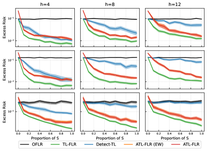
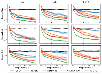
In this section, we explore how the smoothness of the coefficient functions, β(t)\beta^{(t)}, for t𝒮ct\in\mathcal{S}^{c}, will affect the performance of ATL-FLR. We also explore how different temperatures will affect the performance of Exponential Weighted ATL-FLR (ATL-FLR (EW)).

We consider the setting that β(t)\beta^{(t)} with t𝒮ct\in\mathcal{S}^{c} are generated from a much rougher Gaussian process, i.e. βt\beta_{t} are generated from a Gaussian process with mean function cos(2πt)\cos(2\pi t) with covariance kernel min(s,t)\min(s,t), which is exactly Wiener process, and thus the βt\beta_{t}s are less smooth than βt\beta_{t}s that are generated from Ornstein–Uhlenbeck process (the one we used in main paper). For ATL-FLR (EW), we consider three different temperatures, i.e. T=0.2,2,10T=0.2,2,10, where a lower temperature will usually produce small aggregation coefficients. All the other settings are the same as the simulation section.

The results are presented in Figure 3. In general, the patterns of using the Wiener process are consistent with using the Ornstein–Uhlenbeck process, which demonstrates the robustness of the proposed algorithms to negative transfer source models. We also note that while the temperature is low (T=0.2T=0.2), the small convex combination coefficients {cj}\{c_{j}\} will make ATL-FLR(EW) have almost the same performance as ATL-FLR, but it still cannot beat ATL-FLR. While we increase the temperature (T=2,T=10T=2,T=10), the gap between ATL-FLR(EW) and ATL-FLR increases, especially when the proportion of |𝒮||\mathcal{S}| is small. Therefore, selecting the wrong TT can hugely degrade the performance of ATL-FLR(EW). This demonstrates the superiority of sparse aggregation in practice since its performance does not depend on the selection of any hyperparameters.

Refer to caption
(a)
Refer to caption
(b)
Refer to caption
(c)
Figure 3: Excess Risk of different transfer learning algorithms. Each row corresponds to different β(0)\beta^{(0)} and the y-axes for each row are under the same scale. The result for each sample size is an average of 100 replicate experiments with the shaded area indicating ±\pm 2 standard error.

Appendix F Appendix: Real Data Application

In this section, we demonstrate an application of the proposed algorithms in the financial market. The goal of portfolio management is to balance future stock returns and risk, and thus investors can rebalance their portfolios according to their goals. Some investors may be interested in predicting the future stock returns in a specific sector, and transfer learning can borrow market information from other sectors to improve the prediction of the interest.

In this stock data application, for two given adjacent months, we focus on utilizing the Monthly Cumulative Return (MCR) of the first month to predict the Monthly Return (MR) of the subsequent month and improving the prediction accuracy on a certain sector by transferring market information from other sectors. Specifically, suppose for a specific stock, the daily price for the first month is {s1(t0),s1(t1),,s1(tm)}\{s^{1}(t_{0}),s^{1}(t_{1}),\cdots,s^{1}(t_{m})\} and for the second month is {s2(t0),s2(t1),,s2(tm)}\{s^{2}(t_{0}),s^{2}(t_{1}),\cdots,s^{2}(t_{m})\}, then the predictors and responses are expressed as

X(t)=s1(t)s1(t0)s1(t0)andY=s2(tm)s2(t0)s2(t0).X(t)=\frac{s^{1}(t)-s^{1}(t_{0})}{s^{1}(t_{0})}\quad\text{and}\quad Y=\frac{s^{2}(t_{m})-s^{2}(t_{0})}{s^{2}(t_{0})}. (13)

The stock price data are collected from Yahoo Finance (https://finance.yahoo.com/) and we focus on stocks whose corresponding companies have a market cap over 2020 Billion. We divide the sectors based on the division criteria on Nasdaq (https://www.nasdaq.com/market-activity/stocks/screener). The raw data obtained from websites are processed to match the format in (13) and both the raw data and processed data are available in https://github.com/haotianlin/TL-FLM.

After pre-processing, the dataset consists of total 1111 sectors: Basic Industries (BI), Capital Goods (CG), Consumer Durable (CD), Consumer Non-Durable (CND), Consumer Services (CS), Energy (E), Finance (Fin), Health Care (HC), Public Utility (PU), Technology (Tech), and Transportation (Trans), with the number of stocks in each sector as 60,58,31,30,104,55,70,68,46,103,4160,58,31,30,104,55,70,68,46,103,41. The period of the stocks’ price is 05/01/2021 to 09/30/2021.

We compare the performance of Pooled Transfer (Pooled-TL), Naive Transfer (Naive-TL), Detect-TL, ATL-FLR(EW) and ATL-FLR. Naive-TL implements TL-FLR by setting all source sectors belonging to 𝒮\mathcal{S}, while the Pooled-TL one omits the calibrate step in Naive-TL, and the other three are the same as the former simulation section. The learning of each sector is treated as the target task each time, and all the other sectors are sources. We randomly split the target sector into the train (80%80\%) and test (20%20\%) set and report the ratio of the four approaches’ prediction errors to OFLR’s on the test set. We consider the Matérn kernel as the reproducing kernel KK again. Specifically, we set ρ=1\rho=1 and ν=1/2,3/2,\nu=1/2,3/2,\infty (where ν=1/2\nu=1/2 is equivalent to the exponential kernel and ν=\nu=\infty is equivalent to Gaussian kernel) which endows KK with different smoothness properties. The tuning parameters are selected via Generalized Cross-Validation(GCV). Again, we replicate the experiment 100100 times and report the average prediction error with standard error in Figure 4.

Refer to caption
(a)
Refer to caption
(b)
Refer to caption
(c)
Figure 4: Relative prediction error of Pooled-TL, Naive-TL, Detect-TL, ATL-FLR(EW), and ATL-FLR to OFLR for each target sector. Each bar is an average of 100 replications, with standard error as the black line.

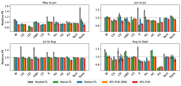
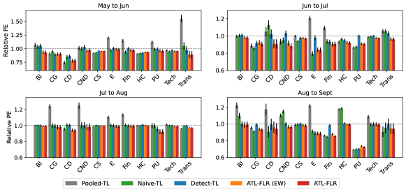
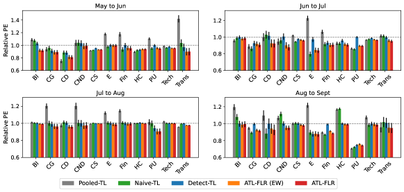
First, we note that the Pooled-TL and Naive-TL only reduce the prediction error in a few sectors, but make no improvement or even downgrade the predictions in most sectors. This implies the effect of direct transfer learning can be quite random, as it can benefit the prediction of the target sector when it shares high similarities with other sectors while having worse performance when similarities are low. Besides, Naive-TL shows an overall better performance compared to the Pooled-TL, demonstrating the importance of the calibrate step. For Detect-TL, all the ratios are close to 11, showing its limited improvement, which is as expected as it can miss positive transfer sources easily. Finally, both ATL-FLR(EW) and ATL-FLR provide more robust improvements on average. We can see both of them have improvements across almost all the sectors, regardless of the similarity between the target sector and source sectors. Comparing the results from different kernels, we can see the improvement patterns are consistent across all the sectors and adjacent months, showing the proposed algorithms are also robust to different reproducing kernels.