This paper was converted on www.awesomepapers.org from LaTeX by an anonymous user.
Want to know more? Visit the Converter page.

On Limiting Likelihood Ratio Processes
of some Change-Point Type Statistical Models

Sergueï Dachian
Laboratoire de Mathématiques
Université Blaise Pascal
63177 Aubière CEDEX, France
Serguei.Dachian@math.univ-bpclermont.fr
Abstract

Different change-point type models encountered in statistical inference for stochastic processes give rise to different limiting likelihood ratio processes. In this paper we consider two such likelihood ratios. The first one is an exponential functional of a two-sided Poisson process driven by some parameter, while the second one is an exponential functional of a two-sided Brownian motion. We establish that for sufficiently small values of the parameter, the Poisson type likelihood ratio can be approximated by the Brownian type one. As a consequence, several statistically interesting quantities (such as limiting variances of different estimators) related to the first likelihood ratio can also be approximated by those related to the second one. Finally, we discuss the asymptotics of the large values of the parameter and illustrate the results by numerical simulations.


Keywords: non-regularity, change-point, limiting likelihood ratio process, Bayesian estimators, maximum likelihood estimator, limiting distribution, limiting variance, asymptotic efficiency


Mathematics Subject Classification (2000): 62F99, 62M99

1 Introduction

Different change-point type models encountered in statistical inference for stochastic processes give rise to different limiting likelihood ratio processes. In this paper we consider two of these processes. The first one is the random process ZρZ_{\rho} on \mathbb{R} defined by

lnZρ(x)={ρΠ+(x)x,if x0,ρΠ(x)x,if x0,\ln Z_{\rho}(x)=\begin{cases}\vphantom{{\mathchoice{\mbox{$\displaystyle\left)\vrule height=11.5pt,depth=0.0pt,width=0.0pt\right.\n@space$}}{\mbox{$\textstyle\left)\vrule height=11.5pt,depth=0.0pt,width=0.0pt\right.\n@space$}}{\mbox{$\scriptstyle\left)\vrule height=5.63496pt,depth=0.0pt,width=0.0pt\right.\n@space$}}{\mbox{$\scriptscriptstyle\left)\vrule height=2.875pt,depth=0.0pt,width=0.0pt\right.\n@space$}}}}\rho\,\Pi_{+}(x)-x,&\text{if }x\geqslant 0,\\ \vphantom{{\mathchoice{\mbox{$\displaystyle\left)\vrule height=11.5pt,depth=0.0pt,width=0.0pt\right.\n@space$}}{\mbox{$\textstyle\left)\vrule height=11.5pt,depth=0.0pt,width=0.0pt\right.\n@space$}}{\mbox{$\scriptstyle\left)\vrule height=5.63496pt,depth=0.0pt,width=0.0pt\right.\n@space$}}{\mbox{$\scriptscriptstyle\left)\vrule height=2.875pt,depth=0.0pt,width=0.0pt\right.\n@space$}}}}-\rho\,\Pi_{-}(-x)-x,&\text{if }x\leqslant 0,\\ \end{cases} (1)

where ρ>0\rho>0, and Π+\Pi_{+} and Π\Pi_{-} are two independent Poisson processes on +\mathbb{R}_{+} with intensities 1/(eρ1)1/(e^{\rho}-1) and 1/(1eρ)1/(1-e^{-\rho}) respectively. We also consider the random variables

ζρ=xZρ(x)𝑑xZρ(x)𝑑xandξρ=argsupxZρ(x)\zeta_{\rho}=\frac{\int_{\mathbb{R}}x\,Z_{\rho}(x)\;dx}{\int_{\mathbb{R}}\,Z_{\rho}(x)\;dx}\quad\text{and}\quad\xi_{\rho}=\mathop{\rm argsup}\limits_{x\in\mathbb{R}}Z_{\rho}(x) (2)

related to this process, as well as to their second moments Bρ=𝐄ζρ2B_{\rho}=\mathbf{E}\zeta_{\rho}^{2} and Mρ=𝐄ξρ2M_{\rho}=\mathbf{E}\xi_{\rho}^{2}.

The process ZρZ_{\rho} (up to a linear time change) arises in some non-regular, namely change-point type, statistical models as the limiting likelihood ratio process, and the variables ζρ\zeta_{\rho} and ξρ\xi_{\rho} (up to a multiplicative constant) as the limiting distributions of the Bayesian estimators and of the maximum likelihood estimator respectively. In particular, BρB_{\rho} and MρM_{\rho} (up to the square of the above multiplicative constant) are the limiting variances of these estimators, and the Bayesian estimators being asymptotically efficient, the ratio Eρ=Bρ/MρE_{\rho}=B_{\rho}/M_{\rho} is the asymptotic efficiency of the maximum likelihood estimator in these models.

The main such model is the below detailed model of i.i.d. observations in the situation when their density has a jump (is discontinuous). Probably the first general result about this model goes back to Chernoff and Rubin [1]. Later, it was exhaustively studied by Ibragimov and Khasminskii in [10, Chapter 5] (\bigl{(}see also their previous works [7] and [8])\bigr{)}.


Model 1. Consider the problem of estimation of the location parameter θ\theta based on the observation Xn=(X1,,Xn)X^{n}=(X_{1},\ldots,X_{n}) of the i.i.d. sample from the density f(xθ)f(x-\theta), where the known function ff is smooth enough everywhere except at 0, and in 0 we have

0limx0f(x)=ab=limx0f(x)0.0\neq\lim_{x\uparrow 0}f(x)=a\neq b=\lim_{x\downarrow 0}f(x)\neq 0.

Denote 𝐏θn\mathbf{P}_{\theta}^{n} the distribution (corresponding to the parameter θ\theta) of the observation XnX^{n}. As nn\to\infty, the normalized likelihood ratio process of this model defined by

Zn(u)=d𝐏θ+unnd𝐏θn(Xn)=i=1nf(Xiθun)f(Xiθ)Z_{n}(u)=\frac{d\mathbf{P}_{\theta+\frac{u}{n}}^{n}}{d\mathbf{P}_{\theta}^{n}}(X^{n})=\prod_{i=1}^{n}\frac{f\left(X_{i}-\theta-\frac{u}{n}\right)}{f(X_{i}-\theta)}

converges weakly in the space 𝒟0(,+)\mathcal{D}_{0}(-\infty,+\infty) (the Skorohod space of functions on \mathbb{R} without discontinuities of the second kind and vanishing at infinity) to the process Za,bZ_{a,b} on \mathbb{R} defined by

lnZa,b(u)={ln(ab)Πb(u)(ab)u,if u0,ln(ab)Πa(u)(ab)u,if u0,\ln Z_{a,b}(u)=\begin{cases}\vphantom{{\mathchoice{\mbox{$\displaystyle\left)\vrule height=14.5pt,depth=0.0pt,width=0.0pt\right.\n@space$}}{\mbox{$\textstyle\left)\vrule height=14.5pt,depth=0.0pt,width=0.0pt\right.\n@space$}}{\mbox{$\scriptstyle\left)\vrule height=7.10497pt,depth=0.0pt,width=0.0pt\right.\n@space$}}{\mbox{$\scriptscriptstyle\left)\vrule height=3.625pt,depth=0.0pt,width=0.0pt\right.\n@space$}}}}\ln(\frac{a}{b})\,\Pi_{b}(u)-(a-b)\,u,&\text{if }u\geqslant 0,\\ \vphantom{{\mathchoice{\mbox{$\displaystyle\left)\vrule height=14.5pt,depth=0.0pt,width=0.0pt\right.\n@space$}}{\mbox{$\textstyle\left)\vrule height=14.5pt,depth=0.0pt,width=0.0pt\right.\n@space$}}{\mbox{$\scriptstyle\left)\vrule height=7.10497pt,depth=0.0pt,width=0.0pt\right.\n@space$}}{\mbox{$\scriptscriptstyle\left)\vrule height=3.625pt,depth=0.0pt,width=0.0pt\right.\n@space$}}}}-\ln(\frac{a}{b})\,\Pi_{a}(-u)-(a-b)\,u,&\text{if }u\leqslant 0,\\ \end{cases}

where Πb\Pi_{b} and Πa\Pi_{a} are two independent Poisson processes on +\mathbb{R}_{+} with intensities bb and aa respectively. The limiting distributions of the Bayesian estimators and of the maximum likelihood estimator are given by

ζa,b=uZa,b(u)𝑑uZa,b(u)𝑑uandξa,b=argsupuZa,b(u)\zeta_{a,b}=\frac{\int_{\mathbb{R}}u\,Z_{a,b}(u)\;du}{\int_{\mathbb{R}}\,Z_{a,b}(u)\;du}\quad\text{and}\quad\xi_{a,b}=\mathop{\rm argsup}\limits_{u\in\mathbb{R}}Z_{a,b}(u)

respectively. The convergence of moments also holds, and the Bayesian estimators are asymptotically efficient. So, 𝐄ζa,b2\mathbf{E}\zeta_{a,b}^{2} and 𝐄ξa,b2\mathbf{E}\xi_{a,b}^{2} are the limiting variances of these estimators, and 𝐄ζa,b2/𝐄ξa,b2\mathbf{E}\zeta_{a,b}^{2}/\mathbf{E}\xi_{a,b}^{2} is the asymptotic efficiency of the maximum likelihood estimator.

Now let us note, that up to a linear time change, the process Za,bZ_{a,b} is nothing but the process ZρZ_{\rho} with ρ=|ln(ab)|\rho=\left|\ln(\frac{a}{b})\right|. Indeed, by putting u=xabu=\frac{x}{a-b} we get

lnZa,b(u)\displaystyle\ln Z_{a,b}(u) ={ln(ab)Πb(xab)x,if xab0,ln(ab)Πa(xab)x,if xab0,\displaystyle=\begin{cases}\vphantom{{\mathchoice{\mbox{$\displaystyle\left)\vrule height=14.5pt,depth=0.0pt,width=0.0pt\right.\n@space$}}{\mbox{$\textstyle\left)\vrule height=14.5pt,depth=0.0pt,width=0.0pt\right.\n@space$}}{\mbox{$\scriptstyle\left)\vrule height=7.10497pt,depth=0.0pt,width=0.0pt\right.\n@space$}}{\mbox{$\scriptscriptstyle\left)\vrule height=3.625pt,depth=0.0pt,width=0.0pt\right.\n@space$}}}}\ln(\frac{a}{b})\,\Pi_{b}(\frac{x}{a-b})-x,&\text{if }\frac{x}{a-b}\geqslant 0,\\ \vphantom{{\mathchoice{\mbox{$\displaystyle\left)\vrule height=14.5pt,depth=0.0pt,width=0.0pt\right.\n@space$}}{\mbox{$\textstyle\left)\vrule height=14.5pt,depth=0.0pt,width=0.0pt\right.\n@space$}}{\mbox{$\scriptstyle\left)\vrule height=7.10497pt,depth=0.0pt,width=0.0pt\right.\n@space$}}{\mbox{$\scriptscriptstyle\left)\vrule height=3.625pt,depth=0.0pt,width=0.0pt\right.\n@space$}}}}-\ln(\frac{a}{b})\,\Pi_{a}(-\frac{x}{a-b})-x,&\text{if }\frac{x}{a-b}\leqslant 0,\\ \end{cases}
=lnZρ(x)=lnZρ((ab)u).\displaystyle=\ln Z_{\rho}(x)=\ln Z_{\rho}\bigl{(}(a-b)\,u\bigr{)}.

So, we have

ζa,b=ζρabandξa,b=ξρab,\zeta_{a,b}=\frac{\zeta_{\rho}}{a-b}\quad\text{and}\quad\xi_{a,b}=\frac{\xi_{\rho}}{a-b}\,,

and hence

𝐄ζa,b2=Bρ(ab)2,𝐄ξa,b2=Mρ(ab)2and𝐄ζa,b2𝐄ξa,b2=Eρ.\mathbf{E}\zeta_{a,b}^{2}=\frac{B_{\rho}}{(a-b)^{2}}\;,\quad\mathbf{E}\xi_{a,b}^{2}=\frac{M_{\rho}}{(a-b)^{2}}\quad\text{and}\quad\frac{\mathbf{E}\zeta_{a,b}^{2}}{\mathbf{E}\xi_{a,b}^{2}}=E_{\rho}\,.

Some other models where the process ZρZ_{\rho} arises occur in the statistical inference for inhomogeneous Poisson processes, in the situation when their intensity function has a jump (is discontinuous). In Kutoyants [14, Chapter 5] (\bigl{(}see also his previous work [12])\bigr{)} one can find several examples, one of which is detailed below.


Model 2. Consider the problem of estimation of the location parameter θ]α,β[\theta\in\left]\alpha,\beta\right[, 0<α<β<τ0<\alpha<\beta<\tau, based on the observation XTX^{T} on [0,T][0,T] of the Poisson process with τ\tau-periodic strictly positive intensity function S(t+θ)S(t+\theta), where the known function SS is smooth enough everywhere except at points t+τkt^{*}+\tau k, kk\in\mathbb{Z}, with some t[0,τ]t^{*}\in\left[0,\tau\right], in which we have

0limttS(t)=SS+=limttS(t)0.0\neq\lim_{t\uparrow t^{*}}S(t)=S_{-}\neq S_{+}=\lim_{t\downarrow t^{*}}S(t)\neq 0.

Denote 𝐏θT\mathbf{P}_{\theta}^{T} the distribution (corresponding to the parameter θ\theta) of the observation XTX^{T}. As TT\to\infty, the normalized likelihood ratio process of this model defined by

ZT(u)=d𝐏θ+uTTd𝐏θT(XT)=exp{0TlnSθ+uT(t)Sθ(t)dX(t)0T[Sθ+uT(t)Sθ(t)]𝑑t}Z_{T}(u)=\frac{d\mathbf{P}_{\theta+\frac{u}{T}}^{T}}{d\mathbf{P}_{\theta}^{T}}(X^{T})=\exp\biggl{\{}\int_{0}^{T}\!\!\ln\frac{S_{\theta+\frac{u}{T}}(t)}{S_{\theta}(t)}\,dX(t)-\int_{0}^{T}\!\!\left[S_{\theta+\frac{u}{T}}(t)-S_{\theta}(t)\right]\!dt\biggr{\}}

converges weakly in the space 𝒟0(,+)\mathcal{D}_{0}(-\infty,+\infty) to the process Zτ,S,S+Z_{\tau,S_{-},S_{+}} on \mathbb{R} defined by

lnZτ,S,S+={ln(S+S)ΠS(uτ)(S+S)uτ,if u0,ln(S+S)ΠS+(uτ)(S+S)uτ,if u0,\ln Z_{\tau,S_{-},S_{+}}=\begin{cases}\vphantom{{\mathchoice{\mbox{$\displaystyle\left)\vrule height=14.5pt,depth=0.0pt,width=0.0pt\right.\n@space$}}{\mbox{$\textstyle\left)\vrule height=14.5pt,depth=0.0pt,width=0.0pt\right.\n@space$}}{\mbox{$\scriptstyle\left)\vrule height=7.10497pt,depth=0.0pt,width=0.0pt\right.\n@space$}}{\mbox{$\scriptscriptstyle\left)\vrule height=3.625pt,depth=0.0pt,width=0.0pt\right.\n@space$}}}}\ln\bigl{(}\frac{S_{+}}{S_{-}}\bigr{)}\,\Pi_{S_{-}}\bigl{(}\frac{u}{\tau}\bigr{)}-(S_{+}-S_{-})\,\frac{u}{\tau}\,,&\text{if }u\geqslant 0,\\ \vphantom{{\mathchoice{\mbox{$\displaystyle\left)\vrule height=14.5pt,depth=0.0pt,width=0.0pt\right.\n@space$}}{\mbox{$\textstyle\left)\vrule height=14.5pt,depth=0.0pt,width=0.0pt\right.\n@space$}}{\mbox{$\scriptstyle\left)\vrule height=7.10497pt,depth=0.0pt,width=0.0pt\right.\n@space$}}{\mbox{$\scriptscriptstyle\left)\vrule height=3.625pt,depth=0.0pt,width=0.0pt\right.\n@space$}}}}-\ln\bigl{(}\frac{S_{+}}{S_{-}}\bigr{)}\,\Pi_{S_{+}}\bigl{(}-\frac{u}{\tau}\bigr{)}-(S_{+}-S_{-})\,\frac{u}{\tau}\,,&\text{if }u\leqslant 0,\\ \end{cases}

where ΠS\Pi_{S_{-}} and ΠS+\Pi_{S_{+}} are two independent Poisson processes on +\mathbb{R}_{+} with intensities SS_{-} and S+S_{+} respectively. The limiting distributions of the Bayesian estimators and of the maximum likelihood estimator are given by

ζτ,S,S+=uZτ,S,S+(u)𝑑uZτ,S,S+(u)𝑑uandξτ,S,S+=argsupuZτ,S,S+(u)\zeta_{\tau,S_{-},S_{+}}=\frac{\int_{\mathbb{R}}u\,Z_{\tau,S_{-},S_{+}}(u)\;du}{\int_{\mathbb{R}}\,Z_{\tau,S_{-},S_{+}}(u)\;du}\quad\text{and}\quad\xi_{\tau,S_{-},S_{+}}=\mathop{\rm argsup}\limits_{u\in\mathbb{R}}Z_{\tau,S_{-},S_{+}}(u)

respectively. The convergence of moments also holds, and the Bayesian estimators are asymptotically efficient. So, 𝐄ζτ,S,S+2\mathbf{E}\zeta_{\tau,S_{-},S_{+}}^{2} and 𝐄ξτ,S,S+2\mathbf{E}\xi_{\tau,S_{-},S_{+}}^{2} are the limiting variances of these estimators, and 𝐄ζτ,S,S+2/𝐄ξτ,S,S+2\mathbf{E}\zeta_{\tau,S_{-},S_{+}}^{2}/\mathbf{E}\xi_{\tau,S_{-},S_{+}}^{2} is the asymptotic efficiency of the maximum likelihood estimator.

Now let us note, that up to a linear time change, the process Zτ,S,S+Z_{\tau,S_{-},S_{+}} is nothing but the process ZρZ_{\rho} with ρ=|ln(S+S)|\rho=\bigl{|}\ln\bigl{(}\frac{S_{+}}{S_{-}}\bigr{)}\bigr{|}. Indeed, by putting u=τxS+Su=\frac{\tau x}{S_{+}-S_{-}} we get

Zτ,S,S+(u)=Zρ(x)=Zρ(S+Sτu).Z_{\tau,S_{-},S_{+}}(u)=Z_{\rho}(x)=Z_{\rho}\left(\frac{S_{+}-S_{-}}{\tau}\,u\right).

So, we have

ζτ,S,S+=τζρS+Sandζτ,S,S+=τξρS+S,\zeta_{\tau,S_{-},S_{+}}=\frac{\tau\,\zeta_{\rho}}{S_{+}-S_{-}}\quad\text{and}\quad\zeta_{\tau,S_{-},S_{+}}=\frac{\tau\,\xi_{\rho}}{S_{+}-S_{-}}\,,

and hence

𝐄ζτ,S,S+2=τ2Bρ(S+S)2,𝐄ξτ,S,S+2=τ2Mρ(S+S)2and𝐄ζτ,S,S+2𝐄ξτ,S,S+2=Eρ.\mathbf{E}\zeta_{\tau,S_{-},S_{+}}^{2}=\frac{\tau^{2}\,B_{\rho}}{(S_{+}-S_{-})^{2}}\;,\quad\mathbf{E}\xi_{\tau,S_{-},S_{+}}^{2}=\frac{\tau^{2}\,M_{\rho}}{(S_{+}-S_{-})^{2}}\quad\text{and}\quad\frac{\mathbf{E}\zeta_{\tau,S_{-},S_{+}}^{2}}{\mathbf{E}\xi_{\tau,S_{-},S_{+}}^{2}}=E_{\rho}\,.

The second limiting likelihood ratio process considered in this paper is the random process

Z0(x)=exp{W(x)12|x|},x,Z_{0}(x)=\exp\left\{W(x)-\frac{1}{2}\left|x\right|\right\},\quad x\in\mathbb{R}, (3)

where WW is a standard two-sided Brownian motion. In this case, the limiting distributions of the Bayesian estimators and of the maximum likelihood estimator (up to a multiplicative constant) are given by

ζ0=xZ0(x)𝑑xZ0(x)𝑑xandξ0=argsupxZ0(x)\zeta_{0}=\frac{\int_{\mathbb{R}}x\,Z_{0}(x)\;dx}{\int_{\mathbb{R}}\,Z_{0}(x)\;dx}\quad\text{and}\quad\xi_{0}=\mathop{\rm argsup}\limits_{x\in\mathbb{R}}Z_{0}(x) (4)

respectively, and the limiting variances of these estimators (up to the square of the above multiplicative constant) are B0=𝐄ζ02B_{0}=\mathbf{E}\zeta_{0}^{2} and M0=𝐄ξ02M_{0}=\mathbf{E}\xi_{0}^{2}.

The models where the process Z0Z_{0} arises occur in various fields of statistical inference for stochastic processes. A well-known example is the below detailed model of a discontinuous signal in a white Gaussian noise exhaustively studied by Ibragimov and Khasminskii in [10, Chapter 7.2] (\bigl{(}see also their previous work [9])\bigr{)}, but one can also cite change-point type models of dynamical systems with small noise (\bigl{(}see Kutoyants [12] and [13, Chapter 5])\bigr{)}, those of ergodic diffusion processes (\bigl{(}see Kutoyants [15, Chapter 3])\bigr{)}, a change-point type model of delay equations (\bigl{(}see Küchler and Kutoyants [11])\bigr{)}, an i.i.d. change-point type model (\bigl{(}see Deshayes and Picard [3])\bigr{)}, a model of a discontinuous periodic signal in a time inhomogeneous diffusion (\bigl{(}see Höpfner and Kutoyants [6])\bigr{)}, and so on.


Model 3. Consider the problem of estimation of the location parameter θ]α,β[\theta\in\left]\alpha,\beta\right[, 0<α<β<10<\alpha<\beta<1, based on the observation XεX^{\varepsilon} on [0,1]\left[0,1\right] of the random process satisfying the stochastic differential equation

dXε(t)=1εS(tθ)dt+dW(t),dX^{\varepsilon}(t)=\frac{1}{\varepsilon}\,S(t-\theta)\,dt+dW(t),

where WW is a standard Brownian motion, and SS is a known function having a bounded derivative on ]1,0[]0,1[\left]-1,0\right[\cup\left]0,1\right[ and satisfying

limt0S(t)limt0S(t)=r0.\lim_{t\uparrow 0}S(t)-\lim_{t\downarrow 0}S(t)=r\neq 0.

Denote 𝐏θε\mathbf{P}_{\theta}^{\varepsilon} the distribution (corresponding to the parameter θ\theta) of the observation XεX^{\varepsilon}. As ε0\varepsilon\to 0, the normalized likelihood ratio process of this model defined by

Zε(u)\displaystyle Z_{\varepsilon}(u) =d𝐏θ+ε2uεd𝐏θε(Xε)\displaystyle=\frac{d\mathbf{P}_{\theta+\varepsilon^{2}u}^{\varepsilon}}{d\mathbf{P}_{\theta}^{\varepsilon}}(X^{\varepsilon})
=exp{1ε01[S(tθε2u)S(tθ)]dW(t)\displaystyle=\exp\biggl{\{}\frac{1}{\varepsilon}\int_{0}^{1}\bigl{[}S(t-\theta-\varepsilon^{2}u)-S(t-\theta)\bigr{]}\,dW(t)
12ε201[S(tθε2u)S(tθ)]2dt}\displaystyle\phantom{=\exp\biggl{\{}}-\frac{1}{2\,\varepsilon^{2}}\int_{0}^{1}\bigl{[}S(t-\theta-\varepsilon^{2}u)-S(t-\theta)\bigr{]}^{2}\,dt\biggr{\}}

converges weakly in the space 𝒞0(,+)\mathcal{C}_{0}(-\infty,+\infty) (the space of continuous functions vanishing at infinity equipped with the supremum norm) to the process Z0(r2u)Z_{0}(r^{2}u), uu\in\mathbb{R}. The limiting distributions of the Bayesian estimators and of the maximum likelihood estimator are r2ζ0r^{-2}\zeta_{0} and r2ξ0r^{-2}\xi_{0} respectively. The convergence of moments also holds, and the Bayesian estimators are asymptotically efficient. So, r4B0r^{-4}B_{0} and r4M0r^{-4}M_{0} are the limiting variances of these estimators, and E0E_{0} is the asymptotic efficiency of the maximum likelihood estimator.


Let us also note that Terent’yev in [20] determined explicitly the distribution of ξ0\xi_{0} and calculated the constant M0=26M_{0}=26. These results were taken up by Ibragimov and Khasminskii in [10, Chapter 7.3], where by means of numerical simulation they equally showed that B0=19.5±0.5B_{0}=19.5\pm 0.5, and so E0=0.73±0.03E_{0}=0.73\pm 0.03. Later in [5], Golubev expressed B0B_{0} in terms of the second derivative (with respect to a parameter) of an improper integral of a composite function of modified Hankel and Bessel functions. Finally in [18], Rubin and Song obtained the exact values B0=16ζ(3)B_{0}=16\,\zeta(3) and E0=8ζ(3)/13E_{0}=8\,\zeta(3)/13, where ζ\zeta is Riemann’s zeta function defined by

ζ(s)=n=11ns.\zeta(s)=\sum_{n=1}^{\infty}\frac{1}{n^{s}}\;.

The random variables ζρ\zeta_{\rho} and ξρ\xi_{\rho} and the quantities BρB_{\rho}, MρM_{\rho} and EρE_{\rho}, ρ>0\rho>0, are much less studied. One can cite Pflug [16] for some results about the distribution of the random variables

argsupx+Zρ(x)andargsupxZρ(x)\mathop{\rm argsup}\limits_{x\in\mathbb{R}_{+}}Z_{\rho}(x)\quad\text{and}\quad\mathop{\rm argsup}\limits_{x\in\mathbb{R}_{-}}Z_{\rho}(x)

related to ξρ\xi_{\rho}.

In this paper we establish that the limiting likelihood ratio processes ZρZ_{\rho} and Z0Z_{0} are related. More precisely, we show that as ρ0\rho\to 0, the process Zρ(y/ρ)Z_{\rho}(y/\rho), yy\in\mathbb{R}, converges weakly in the space 𝒟0(,+)\mathcal{D}_{0}(-\infty,+\infty) to the process Z0Z_{0}. So, the random variables ρζρ\rho\,\zeta_{\rho} and ρξρ\rho\,\xi_{\rho} converge weakly to the random variables ζ0\zeta_{0} and ξ0\xi_{0} respectively. We show equally that the convergence of moments of these random variables holds, that is, ρ2Bρ16ζ(3)\rho^{2}B_{\rho}\to 16\,\zeta(3), ρ2Mρ26\rho^{2}M_{\rho}\to 26 and Eρ8ζ(3)/13E_{\rho}\to 8\,\zeta(3)/13.

These are the main results of the present paper, and they are presented in Section 2, where we also briefly discuss the second possible asymptotics ρ+\rho\to+\infty. The necessary lemmas are proved in Section 3. Finally, some numerical simulations of the quantities BρB_{\rho}, MρM_{\rho} and EρE_{\rho} for ρ]0,[\rho\in\left]0,\infty\right[ are presented in Section 4.

2 Main results

Consider the process Xρ(y)=Zρ(y/ρ)X_{\rho}(y)=Z_{\rho}(y/\rho), yy\in\mathbb{R}, where ρ>0\rho>0 and ZρZ_{\rho} is defined by (1). Note that

yXρ(y)𝑑yXρ(y)𝑑y=ρζρandargsupyXρ(y)=ρξρ,\frac{\int_{\mathbb{R}}y\,X_{\rho}(y)\;dy}{\int_{\mathbb{R}}\,X_{\rho}(y)\;dy}=\rho\,\zeta_{\rho}\quad\text{and}\quad\mathop{\rm argsup}\limits_{y\in\mathbb{R}}X_{\rho}(y)=\rho\,\xi_{\rho}\,,

where the random variables ζρ\zeta_{\rho} and ξρ\xi_{\rho} are defined by (2). Remind also the process Z0Z_{0} on \mathbb{R} defined by (3) and the random variables ζ0\zeta_{0} and ξ0\xi_{0} defined by (4). Recall finally the quantities Bρ=𝐄ζρ2B_{\rho}=\mathbf{E}\zeta_{\rho}^{2}, Mρ=𝐄ξρ2M_{\rho}=\mathbf{E}\xi_{\rho}^{2}, Eρ=Bρ/MρE_{\rho}=B_{\rho}/M_{\rho}, B0=𝐄ζ02=16ζ(3)B_{0}=\mathbf{E}\zeta_{0}^{2}=16\,\zeta(3), M0=𝐄ξ02=26M_{0}=\mathbf{E}\xi_{0}^{2}=26 and E0=B0/M0=8ζ(3)/13E_{0}=B_{0}/M_{0}=8\,\zeta(3)/13. Now we can state the main result of the present paper.

Theorem 1

The process XρX_{\rho} converges weakly in the space 𝒟0(,+)\mathcal{D}_{0}(-\infty,+\infty) to the process Z0Z_{0} as ρ0\rho\to 0. In particular, the random variables ρζρ\rho\,\zeta_{\rho} and ρξρ\rho\,\xi_{\rho} converge weakly to the random variables ζ0\zeta_{0} and ξ0\xi_{0} respectively. Moreover, for any k>0k>0 we have

ρk𝐄ζρk𝐄ζ0kandρk𝐄ξρk𝐄ξ0k,\rho^{k}\,\mathbf{E}\zeta_{\rho}^{k}\to\mathbf{E}\zeta_{0}^{k}\quad\text{and}\quad\rho^{k}\,\mathbf{E}\xi_{\rho}^{k}\to\mathbf{E}\xi_{0}^{k},

and in particular ρ2Bρ16ζ(3)\rho^{2}B_{\rho}\to 16\,\zeta(3), ρ2Mρ26\rho^{2}M_{\rho}\to 26 and Eρ8ζ(3)/13E_{\rho}\to 8\,\zeta(3)/13.

The results concerning the random variable ζρ\zeta_{\rho} are direct consequence of Ibragimov and Khasminskii [10, Theorem 1.10.2] and the following three lemmas.

Lemma 2

The finite-dimensional distributions of the process XρX_{\rho} converge to those of Z0Z_{0} as ρ0\rho\to 0.

Lemma 3

For all ρ>0\rho>0 and all y1,y2y_{1},y_{2}\in\mathbb{R} we have

𝐄|Xρ1/2(y1)Xρ1/2(y2)|214|y1y2|.\mathbf{E}\left|X_{\rho}^{1/2}(y_{1})-X_{\rho}^{1/2}(y_{2})\right|^{2}\leqslant\frac{1}{4}\left|y_{1}-y_{2}\right|.
Lemma 4

For any c] 0, 1/8[c\in\left]\,0\,{,}\;1/8\,\right[ we have

𝐄Xρ1/2(y)exp(c|y|)\mathbf{E}X_{\rho}^{1/2}(y)\leqslant\exp\bigl{(}-c\left|y\right|\bigr{)}

for all sufficiently small ρ\rho and all yy\in\mathbb{R}.

Note that these lemmas are not sufficient to establish the weak convergence of the process XρX_{\rho} in the space 𝒟0(,+)\mathcal{D}_{0}(-\infty,+\infty) and the results concerning the random variable ξρ\xi_{\rho}. However, the increments of the process lnXρ\ln X_{\rho} being independent, the convergence of its restrictions (and hence of those of XρX_{\rho}) on finite intervals [A,B][A,B]\subset\mathbb{R} (\bigl{(}that is, convergence in the Skorohod space 𝒟[A,B]\mathcal{D}[A,B] of functions on [A,B][A,B] without discontinuities of the second kind)\bigr{)} follows from Gihman and Skorohod [4, Theorem 6.5.5], Lemma 2 and the following lemma.

Lemma 5

For any ε>0\varepsilon>0 we have

limh0limρ0sup|y1y2|<h𝐏{|lnXρ(y1)lnXρ(y2)|>ε}=0.\lim_{h\to 0}\ \lim_{\rho\to 0}\ \sup_{\left|y_{1}-y_{2}\right|<h}\mathbf{P}\Bigl{\{}\bigl{|}\ln X_{\rho}(y_{1})-\ln X_{\rho}(y_{2})\bigr{|}>\varepsilon\Bigr{\}}=0.

Now, Theorem 1 follows from the following estimate on the tails of the process XρX_{\rho} by standard argument.

Lemma 6

For any b] 0, 3/40[b\in\left]\,0\,{,}\;3/40\,\right[ we have

𝐏{sup|y|>AXρ(y)>ebA}2ebA\mathbf{P}\biggl{\{}\sup_{\left|y\right|>A}X_{\rho}(y)>e^{-bA}\biggr{\}}\leqslant 2\,e^{-bA}

for all sufficiently small ρ\rho and all A>0A>0.

All the above lemmas will be proved in the next section, but before let us discuss the second possible asymptotics ρ+\rho\to+\infty. One can show that in this case, the process ZρZ_{\rho} converges weakly in the space 𝒟0(,+)\mathcal{D}_{0}(-\infty,+\infty) to the process Z(u)=eu𝟙{u>η}Z_{\infty}(u)=e^{-u}\,\mathbb{1}_{\{u>\eta\}}, uu\in\mathbb{R}, where η\eta is a negative exponential random variable with 𝐏{η<t}=et\mathbf{P}\{\eta<t\}=e^{t}, t0t\leqslant 0. So, the random variables ζρ\zeta_{\rho} and ξρ\xi_{\rho} converge weakly to the random variables

ζ=uZ(u)𝑑uZ(u)𝑑u=η+1andξ=argsupuZ(u)=η\zeta_{\infty}=\frac{\int_{\mathbb{R}}u\,Z_{\infty}(u)\;du}{\int_{\mathbb{R}}\,Z_{\infty}(u)\;du}=\eta+1\quad\text{and}\quad\xi_{\infty}=\mathop{\rm argsup}\limits_{u\in\mathbb{R}}Z_{\infty}(u)=\eta

respectively. One can equally show that, moreover, for any k>0k>0 we have

𝐄ζρk𝐄ζkand𝐄ξρk𝐄ξk,\mathbf{E}\zeta_{\rho}^{k}\to\mathbf{E}\zeta_{\infty}^{k}\quad\text{and}\quad\mathbf{E}\xi_{\rho}^{k}\to\mathbf{E}\xi_{\infty}^{k},

and in particular, denoting B=𝐄ζ2B_{\infty}\!=\mathbf{E}\zeta_{\infty}^{2}, M=𝐄ξ2M_{\infty}\!=\mathbf{E}\xi_{\infty}^{2} and E=B/ME_{\infty}\!=B_{\infty}/M_{\infty}, we finally have BρB=𝐄(η+1)2=1B_{\rho}\to B_{\infty}\!=\mathbf{E}(\eta+1)^{2}=1, MρM=𝐄η2=2M_{\rho}\to M_{\infty}\!=\mathbf{E}\eta^{2}=2 and EρE=1/2E_{\rho}\to E_{\infty}\!=1/2.

Let us note that these convergences are natural, since the process ZZ_{\infty} can be considered as a particular case of the process ZρZ_{\rho} with ρ=+\rho=+\infty if one admits the convention +0=0+\infty\cdot 0=0.

Note also that the process ZZ_{\infty} (up to a linear time change) is the limiting likelihood ratio process of Model 1 (Model 2) in the situation when ab=0a\cdot b=0 (SS+S_{-}\cdot S_{+}=0). In this case, the variables ζ=η+1\zeta_{\infty}=\eta+1 and ξ=η\xi_{\infty}=\eta (up to a multiplicative constant) are the limiting distributions of the Bayesian estimators and of the maximum likelihood estimator respectively. In particular, B=1B_{\infty}=1 and M=2M_{\infty}=2 (up to the square of the above multiplicative constant) are the limiting variances of these estimators, and the Bayesian estimators being asymptotically efficient, E=1/2E_{\infty}=1/2 is the asymptotic efficiency of the maximum likelihood estimator.

3 Proofs of the lemmas

First we prove Lemma 2. Note that the restrictions of the process lnXρ\ln X_{\rho} (as well as those of the process lnZ0\ln Z_{0}) on +\mathbb{R}_{+} and on \mathbb{R}_{-} are mutually independent processes with stationary and independent increments. So, to obtain the convergence of all the finite-dimensional distributions, it is sufficient to show the convergence of one-dimensional distributions only, that is,

lnXρ(y)lnZ0(y)=W(y)|y|2=𝒩(|y|2,|y|)\ln X_{\rho}(y)\Rightarrow\ln Z_{0}(y)=W(y)-\frac{\left|y\right|}{2}=\mathcal{N}\Bigl{(}-\frac{\left|y\right|}{2}\,,\left|y\right|\Bigr{)}

for all yy\in\mathbb{R}. Here and in the sequel “\Rightarrow” denotes the weak convergence of the random variables, and 𝒩(m,V)\mathcal{N}(m,V) denotes a “generic” random variable distributed according to the normal law with mean mm and variance VV.

Let y>0y>0. Then, noting that Π+(yρ)\displaystyle\Pi_{+}\Bigl{(}\frac{y}{\rho}\Bigr{)} is a Poisson random variable of parameter λ=yρ(eρ1)\displaystyle\lambda=\frac{y}{\rho\,(e^{\rho}-1)}\to\infty, we have

lnXρ(y)\displaystyle\ln X_{\rho}(y) =ρΠ+(yρ)yρ=ρyρ(eρ1)Π+(yρ)λλ+yeρ1yρ\displaystyle=\rho\,\Pi_{+}\Bigl{(}\frac{y}{\rho}\Bigr{)}-\frac{y}{\rho}=\rho\,\sqrt{\frac{y}{\rho\,(e^{\rho}-1)}}\ \frac{\Pi_{+}\bigl{(}\frac{y}{\rho}\bigr{)}-\lambda}{\sqrt{\lambda}}+\frac{y}{e^{\rho}-1}-\frac{y}{\rho}
=yρeρ1Π+(yρ)λλyeρ1ρρ(eρ1)𝒩(y2,y),\displaystyle=\sqrt{y}\,\sqrt{\frac{\rho}{e^{\rho}-1}}\ \frac{\Pi_{+}\bigl{(}\frac{y}{\rho}\bigr{)}-\lambda}{\sqrt{\lambda}}-y\,\frac{e^{\rho}-1-\rho}{\rho\,(e^{\rho}-1)}\Rightarrow\mathcal{N}\left(-\frac{y}{2}\,,y\right),

since

ρeρ1=ρρ+o(ρ)1,eρ1ρρ(eρ1)=ρ2/2+o(ρ2)ρ(ρ+o(ρ))12\frac{\rho}{e^{\rho}-1}=\frac{\rho}{\rho+o(\rho)}\to 1,\qquad\frac{e^{\rho}-1-\rho}{\rho\,(e^{\rho}-1)}=\frac{\rho^{2}/2+o(\rho^{2})}{\rho\,\bigr{(}\rho+o(\rho)\bigr{)}}\to\frac{1}{2}

and

Π+(yρ)λλ𝒩(0,1).\frac{\Pi_{+}\bigl{(}\frac{y}{\rho}\bigr{)}-\lambda}{\sqrt{\lambda}}\Rightarrow\mathcal{N}(0,1).

Similarly, for y<0y<0 we have

lnXρ(y)\displaystyle\ln X_{\rho}(y) =ρΠ(yρ)yρ=ρyρ(1eρ)λΠ(yρ)λy1eρyρ\displaystyle=-\rho\,\Pi_{-}\Bigl{(}\frac{-y}{\rho}\Bigr{)}-\frac{y}{\rho}=\rho\,\sqrt{\frac{-y}{\rho\,(1-e^{-\rho})}}\ \frac{\lambda^{\prime}-\Pi_{-}\bigl{(}\frac{-y}{\rho}\bigr{)}}{\sqrt{\lambda^{\prime}}}-\frac{-y}{1-e^{-\rho}}-\frac{y}{\rho}
=yρ1eρλΠ(yρ)λ+yeρ1+ρρ(1eρ)𝒩(y2,y),\displaystyle=\sqrt{-y}\,\sqrt{\frac{\rho}{1-e^{-\rho}}}\ \frac{\lambda^{\prime}-\Pi_{-}\bigl{(}\frac{-y}{\rho}\bigr{)}}{\sqrt{\lambda^{\prime}}}+y\,\frac{e^{-\rho}-1+\rho}{\rho\,(1-e^{-\rho})}\Rightarrow\mathcal{N}\left(\frac{y}{2}\,,-y\right),

and so, Lemma 2 is proved.


Now we turn to the proof of Lemma 4 (we will prove Lemma 3 just after). For y>0y>0 we can write

𝐄Xρ1/2(y)=𝐄exp(ρ2Π+(yρ)y2ρ)=exp(y2ρ)𝐄exp(ρ2Π+(yρ)).\mathbf{E}X_{\rho}^{1/2}(y)=\mathbf{E}\exp\left(\frac{\rho}{2}\,\Pi_{+}\Bigl{(}\frac{y}{\rho}\Bigr{)}-\frac{y}{2\rho}\right)=\exp\left(-\frac{y}{2\rho}\right)\,\mathbf{E}\exp\left(\frac{\rho}{2}\,\Pi_{+}\Bigl{(}\frac{y}{\rho}\Bigr{)}\right).

Note that Π+(yρ)\displaystyle\Pi_{+}\Bigl{(}\frac{y}{\rho}\Bigr{)} is a Poisson random variable of parameter λ=yρ(eρ1)\displaystyle\lambda=\frac{y}{\rho\,(e^{\rho}-1)} with moment generating function M(t)=exp(λ(et1))M(t)=\exp\bigl{(}\lambda\,(e^{t}-1)\bigr{)}. So, we get

𝐄Xρ1/2(y)\displaystyle\mathbf{E}X_{\rho}^{1/2}(y) =exp(y2ρ)exp(yρ(eρ1)(eρ/21))\displaystyle=\exp\left(-\frac{y}{2\rho}\right)\,\exp\left(\frac{y}{\rho\,(e^{\rho}-1)}\,(e^{\rho/2}-1)\right)
=exp(y2ρ+yρ(eρ/2+1))=exp(yeρ/212ρ(eρ/2+1))\displaystyle=\exp\left(-\frac{y}{2\rho}+\frac{y}{\rho\,(e^{\rho/2}+1)}\right)=\exp\left(-y\,\frac{e^{\rho/2}-1}{2\rho\,(e^{\rho/2}+1)}\right)
=exp(yeρ/4eρ/42ρ(eρ/4+eρ/4))=exp(ytanh(ρ/4)2ρ).\displaystyle=\exp\left(-y\,\frac{e^{\rho/4}-e^{-\rho/4}}{2\rho\,(e^{\rho/4}+e^{-\rho/4})}\right)=\exp\left(-y\,\frac{\tanh(\rho/4)}{2\rho}\right).

For y<0y<0 we obtain similarly

𝐄Xρ1/2(y)\displaystyle\mathbf{E}X_{\rho}^{1/2}(y) =𝐄exp(ρ2Π(yρ)y2ρ)\displaystyle=\mathbf{E}\exp\left(-\frac{\rho}{2}\,\Pi_{-}\Bigl{(}\frac{-y}{\rho}\Bigr{)}-\frac{y}{2\rho}\right)
=exp(y2ρ)exp(yρ(1eρ)(eρ/21))\displaystyle=\exp\left(-\frac{y}{2\rho}\right)\,\exp\left(\frac{-y}{\rho\,(1-e^{-\rho})}\,(e^{-\rho/2}-1)\right)
=exp(y2ρ+yρ(1+eρ/2))=exp(y1eρ/22ρ(1+eρ/2))\displaystyle=\exp\left(-\frac{y}{2\rho}+\frac{y}{\rho\,(1+e^{-\rho/2})}\right)=\exp\left(y\,\frac{1-e^{-\rho/2}}{2\rho\,(1+e^{-\rho/2})}\right)
=exp(ytanh(ρ/4)2ρ).\displaystyle=\exp\left(y\,\frac{\tanh(\rho/4)}{2\rho}\right).

Thus, for all yy\in\mathbb{R} we have

𝐄Xρ1/2(y)=exp(|y|tanh(ρ/4)2ρ),\mathbf{E}X_{\rho}^{1/2}(y)=\exp\left(-\left|y\right|\frac{\tanh(\rho/4)}{2\rho}\right), (5)

and since

tanh(ρ/4)2ρ=ρ/4+o(ρ)2ρ18\frac{\tanh(\rho/4)}{2\rho}=\frac{\rho/4+o(\rho)}{2\rho}\to\frac{1}{8}

as ρ0\rho\to 0, for any c] 0, 1/8[c\in\left]\,0\,{,}\;1/8\,\right[ we have 𝐄Xρ1/2(y)exp(c|y|)\mathbf{E}X_{\rho}^{1/2}(y)\leqslant\exp\bigl{(}-c\left|y\right|\bigr{)} for all sufficiently small ρ\rho and all yy\in\mathbb{R}. Lemma 4 is proved.


Further we verify Lemma 3. We first consider the case y1,y2+y_{1},y_{2}\in\mathbb{R}_{+} (say y1y2y_{1}\geqslant y_{2}). Using (5) and taking into account the stationarity and the independence of the increments of the process lnXρ\ln X_{\rho} on +\mathbb{R}_{+}, we can write

𝐄|Xρ1/2(y1)Xρ1/2(y2)|2\displaystyle\mathbf{E}\left|X_{\rho}^{1/2}(y_{1})-X_{\rho}^{1/2}(y_{2})\right|^{2} =𝐄Xρ(y1)+𝐄Xρ(y2)2𝐄Xρ1/2(y1)Xρ1/2(y2)\displaystyle=\mathbf{E}X_{\rho}(y_{1})+\mathbf{E}X_{\rho}(y_{2})-2\,\mathbf{E}X_{\rho}^{1/2}(y_{1})X_{\rho}^{1/2}(y_{2})
=22𝐄Xρ(y2)𝐄Xρ1/2(y1)Xρ1/2(y2)\displaystyle=2-2\,\mathbf{E}X_{\rho}(y_{2})\,\mathbf{E}\frac{X_{\rho}^{1/2}(y_{1})}{X_{\rho}^{1/2}(y_{2})}
=22𝐄Xρ1/2(y1y2)\displaystyle=2-2\,\mathbf{E}X_{\rho}^{1/2}(y_{1}-y_{2})
=22exp(|y1y2|tanh(ρ/4)2ρ)\displaystyle=2-2\exp\left(-\left|y_{1}-y_{2}\right|\frac{\tanh(\rho/4)}{2\rho}\right)
|y1y2|tanh(ρ/4)ρ14|y1y2|.\displaystyle\leqslant\left|y_{1}-y_{2}\right|\frac{\tanh(\rho/4)}{\rho}\leqslant\frac{1}{4}\left|y_{1}-y_{2}\right|.

The case y1,y2y_{1},y_{2}\in\mathbb{R}_{-} can be treated similarly.

Finally, if y1y20y_{1}y_{2}\leqslant 0 (say y20y1y_{2}\leqslant 0\leqslant y_{1}), we have

𝐄|Xρ1/2(y1)Xρ1/2(y2)|2\displaystyle\mathbf{E}\left|X_{\rho}^{1/2}(y_{1})-X_{\rho}^{1/2}(y_{2})\right|^{2} =22𝐄Xρ1/2(y1)𝐄Xρ1/2(y2)\displaystyle=2-2\,\mathbf{E}X_{\rho}^{1/2}(y_{1})\,\mathbf{E}X_{\rho}^{1/2}(y_{2})
=22exp(|y1|tanh(ρ/4)2ρ|y2|tanh(ρ/4)2ρ)\displaystyle=2-2\exp\left(-\left|y_{1}\right|\frac{\tanh(\rho/4)}{2\rho}-\left|y_{2}\right|\frac{\tanh(\rho/4)}{2\rho}\right)
=22exp(|y1y2|tanh(ρ/4)2ρ)\displaystyle=2-2\exp\left(-\left|y_{1}-y_{2}\right|\frac{\tanh(\rho/4)}{2\rho}\right)
14|y1y2|,\displaystyle\leqslant\frac{1}{4}\left|y_{1}-y_{2}\right|,

and so, Lemma 3 is proved.


Now let us check Lemma 5. First let y1,y2+y_{1},y_{2}\in\mathbb{R}_{+} (say y1y2y_{1}\geqslant y_{2}) such that Δ=|y1y2|<h\Delta=\left|y_{1}-y_{2}\right|<h. Then

𝐏{|lnXρ(y1)lnXρ(y2)|>ε}\displaystyle\mathbf{P}\Bigl{\{}\bigl{|}\ln X_{\rho}(y_{1})-\ln X_{\rho}(y_{2})\bigr{|}>\varepsilon\Bigr{\}} 1ε2𝐄|lnXρ(y1)lnXρ(y2)|2\displaystyle\leqslant\frac{1}{\varepsilon^{2}}\,\mathbf{E}\bigl{|}\ln X_{\rho}(y_{1})-\ln X_{\rho}(y_{2})\bigr{|}^{2}
=1ε2𝐄|lnXρ(Δ)|2\displaystyle=\frac{1}{\varepsilon^{2}}\,\mathbf{E}\bigl{|}\ln X_{\rho}(\Delta)\bigr{|}^{2}
=1ε2𝐄|ρΠ+(Δρ)Δρ|2\displaystyle=\frac{1}{\varepsilon^{2}}\,\mathbf{E}\left|\rho\,\Pi_{+}\Bigl{(}\frac{\Delta}{\rho}\Bigr{)}-\frac{\Delta}{\rho}\right|^{2}
=1ε2(ρ2(λ+λ2)+Δ2ρ22λΔ)\displaystyle=\frac{1}{\varepsilon^{2}}\left(\rho^{2}(\lambda+\lambda^{2})+\frac{\Delta^{2}}{\rho^{2}}-2\lambda\Delta\right)
=1ε2(β(ρ)Δ+γ(ρ)Δ2)\displaystyle=\frac{1}{\varepsilon^{2}}\left(\beta(\rho)\,\Delta+\gamma(\rho)\,\Delta^{2}\right)
<1ε2(β(ρ)h+γ(ρ)h2),\displaystyle<\frac{1}{\varepsilon^{2}}\left(\beta(\rho)\,h+\gamma(\rho)\,h^{2}\right),

where λ=Δρ(eρ1)\lambda=\frac{\Delta}{\rho\,(e^{\rho}-1)} is the parameter of the Poisson random variable Π+(Δρ)\Pi_{+}\bigl{(}\!\frac{\Delta}{\rho}\!\bigr{)},

β(ρ)\displaystyle\beta(\rho) =ρ(eρ1)=ρρ+o(ρ)1\displaystyle=\frac{\rho}{(e^{\rho}-1)}=\frac{\rho}{\rho+o(\rho)}\to 1
and
γ(ρ)\displaystyle\gamma(\rho) =1(eρ1)2+1ρ22ρ(eρ1)=(1ρ1eρ1)2\displaystyle=\frac{1}{(e^{\rho}-1)^{2}}+\frac{1}{\rho^{2}}-\frac{2}{\rho\,(e^{\rho}-1)}=\left(\frac{1}{\rho}-\frac{1}{e^{\rho}-1}\right)^{2}
=(eρ1ρρ(eρ1))2=(ρ2/2+o(ρ2)ρ(ρ+o(ρ)))214\displaystyle=\biggl{(}\frac{e^{\rho}-1-\rho}{\rho\,(e^{\rho}-1)}\biggr{)}^{2}=\biggl{(}\frac{\rho^{2}/2+o(\rho^{2})}{\rho\,\bigl{(}\rho+o(\rho)\bigr{)}}\biggr{)}^{2}\to\frac{1}{4}

as ρ0\rho\to 0. So, we have

limρ0sup|y1y2|<h𝐏{|lnXρ(y1)lnXρ(y2)|>ε}\displaystyle\lim_{\rho\to 0}\ \sup_{\left|y_{1}-y_{2}\right|<h}\mathbf{P}\Bigl{\{}\bigl{|}\ln X_{\rho}(y_{1})-\ln X_{\rho}(y_{2})\bigr{|}>\varepsilon\Bigr{\}} limρ01ε2(β(ρ)h+γ(ρ)h2)\displaystyle\leqslant\lim_{\rho\to 0}\frac{1}{\varepsilon^{2}}\left(\beta(\rho)\,h+\gamma(\rho)\,h^{2}\right)
=1ε2(h+h24),\displaystyle=\frac{1}{\varepsilon^{2}}\left(h+\frac{h^{2}}{4}\right),

and hence

limh0limρ0sup|y1y2|<h𝐏{|lnXρ(y1)lnXρ(y2)|>ε}=0,\lim_{h\to 0}\ \lim_{\rho\to 0}\ \sup_{\left|y_{1}-y_{2}\right|<h}\mathbf{P}\Bigl{\{}\bigl{|}\ln X_{\rho}(y_{1})-\ln X_{\rho}(y_{2})\bigr{|}>\varepsilon\Bigr{\}}=0,

where the supremum is taken only over y1,y2+y_{1},y_{2}\in\mathbb{R}_{+}.

For y1,y2y_{1},y_{2}\in\mathbb{R}_{-} such that Δ=|y1y2|<h\Delta=\left|y_{1}-y_{2}\right|<h one can obtain similarly

𝐏{|lnXρ(y1)lnXρ(y2)|>ε}\displaystyle\mathbf{P}\Bigl{\{}\bigl{|}\ln X_{\rho}(y_{1})-\ln X_{\rho}(y_{2})\bigr{|}>\varepsilon\Bigr{\}} 1ε2𝐄|lnXρ(y1)lnXρ(y2)|2\displaystyle\leqslant\frac{1}{\varepsilon^{2}}\,\mathbf{E}\bigl{|}\ln X_{\rho}(y_{1})-\ln X_{\rho}(y_{2})\bigr{|}^{2}
=1ε2(β(ρ)Δ+γ(ρ)Δ2)\displaystyle=\frac{1}{\varepsilon^{2}}\left(\beta^{\prime}(\rho)\,\Delta+\gamma^{\prime}(\rho)\,\Delta^{2}\right)
<1ε2(β(ρ)h+γ(ρ)h2),\displaystyle<\frac{1}{\varepsilon^{2}}\left(\beta^{\prime}(\rho)\,h+\gamma^{\prime}(\rho)\,h^{2}\right),

where

β(ρ)\displaystyle\beta^{\prime}(\rho) =ρ(1eρ)=ρρ+o(ρ)1\displaystyle=\frac{\rho}{(1-e^{-\rho})}=\frac{\rho}{\rho+o(\rho)}\to 1
and
γ(ρ)\displaystyle\gamma^{\prime}(\rho) =(eρ1+ρρ(1eρ))2=(ρ2/2+o(ρ2)ρ(ρ+o(ρ)))214\displaystyle=\biggl{(}\frac{e^{-\rho}-1+\rho}{\rho\,(1-e^{\rho})}\biggr{)}^{2}=\biggl{(}\frac{\rho^{2}/2+o(\rho^{2})}{\rho\,\bigl{(}\rho+o(\rho)\bigr{)}}\biggr{)}^{2}\to\frac{1}{4}

as ρ0\rho\to 0, which will yield the same conclusion as above, but with the supremum taken over y1,y2y_{1},y_{2}\in\mathbb{R}_{-}.

Finally, for y1y20y_{1}y_{2}\leqslant 0 (say y20y1y_{2}\leqslant 0\leqslant y_{1}) such that |y1y2|<h\left|y_{1}-y_{2}\right|<h, using the elementary inequality (ab)22(a2+b2)(a-b)^{2}\leqslant 2(a^{2}+b^{2}) we get

𝐏{|lnXρ(y1)lnXρ(y2)|>ε}\displaystyle\mathbf{P}\Bigl{\{}\bigl{|}\ln X_{\rho}(y_{1})-\ln X_{\rho}(y_{2})\bigr{|}>\varepsilon\Bigr{\}} 1ε2𝐄|lnXρ(y1)lnXρ(y2)|2\displaystyle\leqslant\frac{1}{\varepsilon^{2}}\,\mathbf{E}\bigl{|}\ln X_{\rho}(y_{1})-\ln X_{\rho}(y_{2})\bigr{|}^{2}
2ε2(𝐄|lnXρ(y1)|2+𝐄|lnXρ(y2)|2)\displaystyle\leqslant\frac{2}{\varepsilon^{2}}\left(\mathbf{E}\bigl{|}\ln X_{\rho}(y_{1})\bigr{|}^{2}+\mathbf{E}\bigl{|}\ln X_{\rho}(y_{2})\bigr{|}^{2}\right)
=2ε2(β(ρ)y1+γ(ρ)y12+β(ρ)|y2|+γ(ρ)|y2|2)\displaystyle=\frac{2}{\varepsilon^{2}}\left(\beta(\rho)y_{1}\!+\!\gamma(\rho)y_{1}^{2}\!+\!\beta^{\prime}(\rho)\!\left|y_{2}\right|\!+\!\gamma^{\prime}(\rho)\!\left|y_{2}\right|^{2}\right)
2ε2((β(ρ)+β(ρ))h+(γ(ρ)+γ(ρ))h2),\displaystyle\leqslant\frac{2}{\varepsilon^{2}}\Bigl{(}\bigl{(}\beta(\rho)+\beta^{\prime}(\rho)\bigr{)}\,h+\bigl{(}\gamma(\rho)+\gamma^{\prime}(\rho)\bigr{)}\,h^{2}\Bigr{)},

which again will yield the desired conclusion. Lemma 5 is proved.


It remains to verify Lemma 6. Clearly,

𝐏{sup|y|>AXρ(y)>ebA}𝐏{supy>AXρ(y)>ebA}+𝐏{supy<AXρ(y)>ebA}.\mathbf{P}\biggl{\{}\sup_{\left|y\right|>A}X_{\rho}(y)>e^{-bA}\biggr{\}}\leqslant\mathbf{P}\biggl{\{}\sup_{y>A}X_{\rho}(y)>e^{-bA}\biggr{\}}+\mathbf{P}\biggl{\{}\sup_{y<-A}X_{\rho}(y)>e^{-bA}\biggr{\}}.

In order to estimate the first term, we need two auxiliary results.

Lemma 7

For any c] 0, 3/32[c\in\left]\,0\,{,}\;3/32\,\right[ we have

𝐄Xρ1/4(y)exp(c|y|)\mathbf{E}X_{\rho}^{1/4}(y)\leqslant\exp\bigl{(}-c\left|y\right|\bigr{)}

for all sufficiently small ρ\rho and all yy\in\mathbb{R}.

Lemma 8

For all ρ>0\rho>0 the random variable

ηρ=supt+(Πλ(t)t),\eta_{\rho}=\sup_{t\in\mathbb{R}_{+}}\bigl{(}\Pi_{\lambda}(t)-t\bigr{)},

where Πλ\Pi_{\lambda} is a Poisson process on +\mathbb{R}_{+} with intensity λ=ρ/(eρ1)]0,1[\lambda=\rho/(e^{\rho}-1)\in\left]0,1\right[, verifies

𝐄exp(ρ4ηρ)2.\mathbf{E}\exp\left(\frac{\rho}{4}\,\eta_{\rho}\right)\leqslant 2.

The first result can be easily obtained following the proof of Lemma 4, so we prove the second one only. For this, let us remind that according to Shorack and Wellner [19, Proposition 1 on page 392] (\bigl{(}see also Pyke [17])\bigr{)}, the distribution function Fρ(x)=𝐏{ηρ<x}F_{\rho}(x)=\mathbf{P}\{\eta_{\rho}<x\} of ηρ\eta_{\rho} is given by

1Fρ(x)=𝐏{ηρx}=(1λ)eλxn>x(nx)nn!(λeλ)n1-F_{\rho}(x)=\mathbf{P}\{\eta_{\rho}\geqslant x\}=(1-\lambda)\,e^{\lambda x}\sum_{n>x}\frac{(n-x)^{n}}{n!}\,\bigl{(}\lambda\,e^{-\lambda}\bigr{)}^{n}

for x>0x>0, and is zero for x0x\leqslant 0. Hence, for x>0x>0 we have

1Fρ(x)\displaystyle 1-F_{\rho}(x) (1λ)eλxn>x(nx)n2πnnnen(λeλ)n\displaystyle\leqslant(1-\lambda)\,e^{\lambda x}\,\sum_{n>x}\frac{(n-x)^{n}}{\sqrt{2\pi n}\,n^{n}\,e^{-n}}\,\bigl{(}\lambda\,e^{-\lambda}\bigr{)}^{n}
=1λ2πeλxn>x1n(1xn)n(λe1λ)n\displaystyle=\frac{1-\lambda}{\sqrt{2\pi}}\,e^{\lambda x}\,\sum_{n>x}\frac{1}{\sqrt{n}}\left(1-\frac{x}{n}\right)^{n}\bigl{(}\lambda\,e^{1-\lambda}\bigr{)}^{n}
1λ2πeλxn>xex(λe1λ)nn\displaystyle\leqslant\frac{1-\lambda}{\sqrt{2\pi}}\,e^{\lambda x}\,\sum_{n>x}e^{-x}\frac{\bigl{(}\lambda\,e^{1-\lambda}\bigr{)}^{n}}{\sqrt{n}}
1λ2πe(λ1)x(λe1λ)xn>x(λe1λ)nxnx\displaystyle\leqslant\frac{1-\lambda}{\sqrt{2\pi}}\,e^{(\lambda-1)x}\,\bigl{(}\lambda\,e^{1-\lambda}\bigr{)}^{x}\sum_{n>x}\frac{\bigl{(}\lambda\,e^{1-\lambda}\bigr{)}^{n-x}}{\sqrt{n-x}}
=1λ2πλxk>0(λe1λ)kk1λ2πλx+(λe1λ)tt𝑑t\displaystyle=\frac{1-\lambda}{\sqrt{2\pi}}\,\lambda^{x}\sum_{k>0}\frac{\bigl{(}\lambda\,e^{1-\lambda}\bigr{)}^{k}}{\sqrt{k}}\leqslant\frac{1-\lambda}{\sqrt{2\pi}}\,\lambda^{x}\int_{\mathbb{R}_{+}}\frac{\bigl{(}\lambda\,e^{1-\lambda}\bigr{)}^{t}}{\sqrt{t}}\;dt
=1λ2πλxΓ(1/2)ln(λe1λ)=1λ2ln(λe1λ)(ρeρ1)x\displaystyle=\frac{1-\lambda}{\sqrt{2\pi}}\,\lambda^{x}\,\frac{\Gamma(1/2)}{\sqrt{-\ln\bigl{(}\lambda\,e^{1-\lambda}\bigr{)}}}=\frac{1-\lambda}{\sqrt{-2\ln\bigl{(}\lambda\,e^{1-\lambda}\bigr{)}}}\left(\frac{\rho}{e^{\rho}-1}\right)^{x}
(ρeρ/2eρ/2eρ/2)x=(ρeρ/22sinh(ρ/2))xeρx/2,\displaystyle\leqslant\left(\frac{\rho\,e^{-\rho/2}}{e^{\rho/2}-e^{-\rho/2}}\right)^{x}=\left(\frac{\rho\,e^{-\rho/2}}{2\sinh(\rho/2)}\right)^{x}\leqslant e^{-\rho x/2},

where we used Stirling inequality and the inequality 1λ2ln(λe1λ)1-\lambda\leqslant\sqrt{-2\ln\bigl{(}\lambda\,e^{1-\lambda}\bigr{)}}, which is easily reduced to the elementary inequality ln(1μ)μμ2/2\ln(1-\mu)\leqslant-\mu-\mu^{2}/2 by putting μ=1λ\mu=1-\lambda. So, we can finish the proof of Lemma 8 by writing

𝐄exp(ρ4ηρ)\displaystyle\mathbf{E}\exp\left(\frac{\rho}{4}\,\eta_{\rho}\right) =eρx/4𝑑Fρ(x)\displaystyle=\int_{\mathbb{R}}e^{\,\rho x/4}\;dF_{\rho}(x)
=[eρx/4(Fρ(x)1)]+ρ4eρx/4(Fρ(x)1)𝑑x\displaystyle=\Bigl{[}e^{\,\rho x/4}\bigl{(}F_{\rho}(x)-1\bigr{)}\Bigr{]}_{-\infty}^{+\infty}-\;\frac{\rho}{4}\int_{\mathbb{R}}e^{\,\rho x/4}\bigl{(}F_{\rho}(x)-1\bigr{)}\;dx
=ρ4eρx/4𝑑x+ρ4+eρx/4(1Fρ(x))𝑑x\displaystyle=\frac{\rho}{4}\int_{\mathbb{R}_{-}}e^{\,\rho x/4}\;dx+\frac{\rho}{4}\int_{\mathbb{R}_{+}}e^{\,\rho x/4}\bigl{(}1-F_{\rho}(x)\bigr{)}\;dx
1+ρ4+eρx/4𝑑x=2.\displaystyle\leqslant 1+\frac{\rho}{4}\int_{\mathbb{R}_{+}}e^{-\rho x/4}\;dx=2.

Now, let us get back to the proof of Lemma 6. Using Lemma 8 and taking into account the stationarity and the independence of the increments of the process lnXρ\ln X_{\rho} on +\mathbb{R}_{+}, we obtain

𝐏{supy>AXρ(y)>ebA}\displaystyle\mathbf{P}\biggl{\{}\sup_{y>A}X_{\rho}(y)>e^{-bA}\biggr{\}} ebA/4𝐄supy>AXρ1/4(y)\displaystyle\leqslant e^{\,bA/4}\;\mathbf{E}\sup_{y>A}X_{\rho}^{1/4}(y)
=ebA/4𝐄Xρ1/4(A)𝐄supy>AXρ1/4(y)Xρ1/4(A)\displaystyle=e^{\,bA/4}\;\mathbf{E}X_{\rho}^{1/4}(A)\;\mathbf{E}\sup_{y>A}\frac{X_{\rho}^{1/4}(y)}{X_{\rho}^{1/4}(A)}
=ebA/4𝐄Xρ1/4(A)𝐄supz>0Xρ1/4(z)\displaystyle=e^{\,bA/4}\;\mathbf{E}X_{\rho}^{1/4}(A)\;\mathbf{E}\sup_{z>0}X_{\rho}^{1/4}(z)
=ebA/4𝐄Xρ1/4(A)𝐄supz>0(exp(ρ4Π+(z/ρ)z4ρ))\displaystyle=e^{\,bA/4}\;\mathbf{E}X_{\rho}^{1/4}(A)\;\mathbf{E}\sup_{z>0}\left(\exp\Bigl{(}\frac{\rho}{4}\,\Pi_{+}(z/\rho)-\frac{z}{4\rho}\Bigr{)}\right)
=ebA/4𝐄Xρ1/4(A)𝐄exp(supt>0(ρ4(Πρeρ1(t)t)))\displaystyle=e^{\,bA/4}\;\mathbf{E}X_{\rho}^{1/4}(A)\;\mathbf{E}\exp\left(\sup_{t>0}\Bigl{(}\frac{\rho}{4}\bigl{(}\Pi_{\textstyle\frac{\rho}{e^{\rho}-1}}(t)-t\bigr{)}\Bigr{)}\right)
=ebA/4𝐄Xρ1/4(A)𝐄exp(ρ4ηρ)2ebA/4𝐄Xρ1/4(A).\displaystyle=e^{\,bA/4}\;\mathbf{E}X_{\rho}^{1/4}(A)\;\mathbf{E}\exp\left(\frac{\rho}{4}\,\eta_{\rho}\right)\leqslant 2\,e^{\,bA/4}\;\mathbf{E}X_{\rho}^{1/4}(A).

Hence, taking b] 0, 3/40[b\in\left]\,0\,{,}\;3/40\,\right[, we have 5b/4] 0, 3/32[5b/4\in\left]\,0\,{,}\;3/32\,\right[ and, using Lemma 7, we finally get

𝐏{supy>AXρ(y)>ebA}\displaystyle\mathbf{P}\biggl{\{}\sup_{y>A}X_{\rho}(y)>e^{-bA}\biggr{\}} 2ebA/4exp(5b4A)=2ebA\displaystyle\leqslant 2\,e^{\,bA/4}\,\exp\Bigl{(}-\frac{5b}{4}A\Bigr{)}=2\,e^{-bA}

for all sufficiently small ρ\rho and all A>0A>0, and so the first term is estimated.

The second term can be estimated in the same way, if we show that for all ρ>0\rho>0 the random variable

ηρ=supt+(Πλ(t)+t)=inft+(Πλ(t)t),\eta_{\rho}^{\prime}=\sup_{t\in\mathbb{R}_{+}}\bigl{(}-\Pi_{\lambda^{\prime}}(t)+t\bigr{)}=-\inf_{t\in\mathbb{R}_{+}}\bigl{(}\Pi_{\lambda^{\prime}}(t)-t\bigr{)},

where Πλ\Pi_{\lambda^{\prime}} is a Poisson process on +\mathbb{R}_{+} with intensity λ=ρ/(1eρ)]0,1[\lambda^{\prime}=\rho/(1-e^{-\rho})\in\left]0,1\right[, verifies

𝐄exp(ρ4ηρ)2.\mathbf{E}\exp\left(\frac{\rho}{4}\,\eta_{\rho}^{\prime}\right)\leqslant 2.

For this, let us remind that according to Pyke [17] (\bigl{(}see also Cramér [2])\bigr{)}, ηρ\eta_{\rho}^{\prime} is an exponential random variable with parameter rr, where rr is the unique positive solution of the equation

λ(er1)+r=0.\lambda^{\prime}(e^{-r}-1)+r=0.

In our case, this equation becomes

ρ1eρ(er1)+r=0,\frac{\rho}{1-e^{-\rho}}\,(e^{-r}-1)+r=0,

and r=ρr=\rho is clearly its solution. Hence ηρ\eta_{\rho}^{\prime} is an exponential random variable with parameter ρ\rho, which yields

𝐄exp(ρ4ηρ)=43<2,\mathbf{E}\exp\left(\frac{\rho}{4}\,\eta_{\rho}^{\prime}\right)=\frac{4}{3}<2,

and so, Lemma 6 is proved.

4 Numerical simulations

In this section we present some numerical simulations of the quantities BρB_{\rho}, MρM_{\rho} and EρE_{\rho} for ρ]0,[\rho\in\left]0,\infty\right[. Besides giving approximate values of these quantities, the simulation results illustrate both the asymptotics

BρB0ρ2,MρM0ρ2andEρE0asρ0,B_{\rho}\sim\frac{B_{0}}{\rho^{2}}\,,\quad M_{\rho}\sim\frac{M_{0}}{\rho^{2}}\quad\text{and}\quad E_{\rho}\to E_{0}\quad\text{as}\quad\rho\to 0,

with B0=16ζ(3)19.2329B_{0}=16\,\zeta(3)\approx 19.2329, M0=26M_{0}=26 and E0=8ζ(3)/130.7397E_{0}=8\,\zeta(3)/13\approx 0.7397, and

BρB,MρMandEρEasρ,B_{\rho}\to B_{\infty},\quad M_{\rho}\to M_{\infty}\quad\text{and}\quad E_{\rho}\to E_{\infty}\quad\text{as}\quad\rho\to\infty,

with B=1B_{\infty}=1, M=2M_{\infty}=2 and E=0.5E_{\infty}=0.5.

First, we simulate the events x1,x2,x_{1},x_{2},\ldots of the Poisson process Π+\Pi_{+} (\bigl{(}with the intensity 1/(eρ1))1/(e^{\rho}-1)\bigr{)}, and the events x1,x2,x^{\prime}_{1},x^{\prime}_{2},\ldots of the Poisson process Π\Pi_{-} (\bigl{(}with the intensity 1/(1eρ))1/(1-e^{-\rho})\bigr{)}.

Then we calculate

ζρ\displaystyle\zeta_{\rho} =xZρ(x)𝑑xZρ(x)𝑑x\displaystyle=\frac{\displaystyle\int_{\mathbb{R}}x\,Z_{\rho}(x)\;dx}{\displaystyle\int_{\mathbb{R}}\,Z_{\rho}(x)\;dx}
=i=1xieρixi+i=1eρixii=1xieρρi+xi+i=1eρρi+xii=1eρixi+i=1eρρi+xi\displaystyle=\frac{\displaystyle\sum_{i=1}^{\infty}x_{i}\,e^{\rho i-x_{i}}+\sum_{i=1}^{\infty}e^{\rho i-x_{i}}-\sum_{i=1}^{\infty}x^{\prime}_{i}\,e^{\rho-\rho i+x^{\prime}_{i}}+\sum_{i=1}^{\infty}e^{\rho-\rho i+x^{\prime}_{i}}}{\displaystyle\sum_{i=1}^{\infty}e^{\rho i-x_{i}}+\sum_{i=1}^{\infty}e^{\rho-\rho i+x^{\prime}_{i}}}
and
ξρ\displaystyle\xi_{\rho} =argsupxZρ(x)={xk,if ρkxk>ρρ+x,x,otherwise,\displaystyle=\mathop{\rm argsup}\limits_{x\in\mathbb{R}}Z_{\rho}(x)=\begin{cases}x_{k},&\text{if }\rho k-x_{k}>\rho-\rho\ell+x^{\prime}_{\ell},\\ -x^{\prime}_{\ell},&\text{otherwise},\end{cases}

where

k=argmaxi1(ρixi)and=argmaxi1(ρρi+xi),k=\mathop{\rm argmax}\limits_{i\geqslant 1}\,(\rho i-x_{i})\quad\text{and}\quad\ell=\mathop{\rm argmax}\limits_{i\geqslant 1}\,(\rho-\rho i+x^{\prime}_{i}),

so that

xk=argsupx+Zρ(x)andx=argsupxZρ(x).x_{k}=\mathop{\rm argsup}\limits_{x\in\mathbb{R}_{+}}Z_{\rho}(x)\quad\text{and}\quad-x^{\prime}_{\ell}=\mathop{\rm argsup}\limits_{x\in\mathbb{R}_{-}}Z_{\rho}(x).

Finally, repeating these simulations 10710^{7} times (for each value of ρ\rho), we approximate Bρ=𝐄ζρ2B_{\rho}=\mathbf{E}\zeta_{\rho}^{2} and Mρ=𝐄ξρ2M_{\rho}=\mathbf{E}\xi_{\rho}^{2} by the empirical second moments, and Eρ=Bρ/MρE_{\rho}=B_{\rho}/M_{\rho} by their ratio.

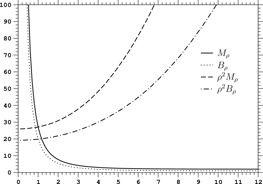
The results of the numerical simulations are presented in Figures 1 and 2. The ρ0\rho\to 0 asymptotics of BρB_{\rho} and MρM_{\rho} can be observed in Figure 1, where besides these functions we also plotted the functions ρ2Bρ\rho^{2}B_{\rho} and ρ2Mρ\rho^{2}M_{\rho}, making apparent the constants B019.2329B_{0}\approx 19.2329 and M0=26M_{0}=26.

Refer to caption
Figure 1: BρB_{\rho} and MρM_{\rho} (ρ0\rho\to 0 asymptotics)

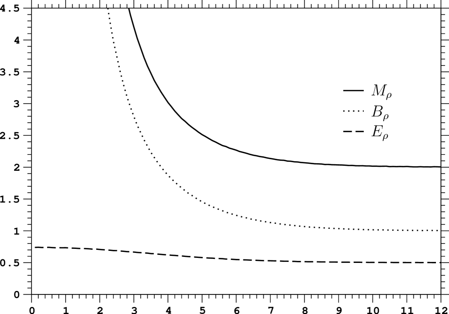
In Figure 2 we use a different scale on the vertical axis to better illustrate the ρ\rho\to\infty asymptotics of BρB_{\rho} and MρM_{\rho}, as well as both the asymptotics of EρE_{\rho}. Note that the function EρE_{\rho} appear to be decreasing, so we can conjecture that bigger is ρ\rho, smaller is the efficiency of the maximum likelihood estimator, and so, this efficiency is always between E=0.5E_{\infty}=0.5 and E00.7397E_{0}\approx 0.7397.

Refer to caption
Figure 2: BρB_{\rho} and MρM_{\rho} (ρ\rho\to\infty asymptotics) EρE_{\rho} (both asymptotics)

References

  • [1] Chernoff, H and Rubin, H, “The estimation of the location of a discontinuity in density”, Proc. 3rd Berkeley Symp. 1, pp. 19–37, 1956.
  • [2] Cramér, H., “On some questions connected with mathematical risk”, Univ. California Publ. Statist. 2, pp. 99–123, 1954.
  • [3] Deshayes, J. and Picard, D., “Lois asymptotiques des tests et estimateurs de rupture dans un modèle statistique classique”, Ann. Inst. H. Poincaré Probab. Statist. 20, no. 4, pp. 309–327, 1984.
  • [4] Gihman, I.I. and Skorohod, A.V., “The theory of stochastic processes I.”, Springer-Verlag, New York, 1974.
  • [5] Golubev, G.K., “Computation of the efficiency of the maximum-likelihood estimator when observing a discontinuous signal in white noise”, Problems Inform. Transmission 15, no. 3, pp. 61–69, 1979.
  • [6] Höpfner, R. and Kutoyants, Yu.A., “Estimating discontinuous periodic signals in a time inhomogeneous diffusion”, preprint, 2009.
    http://www.mathematik.uni-mainz.de/˜hoepfner/ssp/zeit.html
  • [7] Ibragimov, I.A. and Khasminskii, R.Z., “On the asymptotic behavior of generalized Bayes’ estimator”, Dokl. Akad. Nauk SSSR 194, pp. 257–260, 1970.
  • [8] Ibragimov, I.A. and Khasminskii, R.Z., “The asymptotic behavior of statistical estimates for samples with a discontinuous density”, Mat. Sb. 87 (129), no. 4, pp. 554–558, 1972.
  • [9] Ibragimov, I.A. and Khasminskii, R.Z., “Estimation of a parameter of a discontinuous signal in a white Gaussian noise”, Problems Inform. Transmission 11, no. 3, pp. 31–43, 1975.
  • [10] Ibragimov, I.A. and Khasminskii, R.Z., “Statistical estimation. Asymptotic theory”, Springer-Verlag, New York, 1981.
  • [11] Küchler, U. and Kutoyants, Yu.A., “Delay estimation for some stationary diffusion-type processes”, Scand. J. Statist. 27, no. 3, pp. 405–414, 2000.
  • [12] Kutoyants, Yu.A., “Parameter estimation for stochastic processes”, Armenian Academy of Sciences, Yerevan, 1980 (in Russian), translation of revised version, Heldermann-Verlag, Berlin, 1984.
  • [13] Kutoyants, Yu.A., “Identification of dynamical systems with small noise”, Mathematics and its Applications 300, Kluwer Academic Publishers Group, Dordrecht, 1994.
  • [14] Kutoyants, Yu.A., “Statistical Inference for Spatial Poisson Processes”, Lect. Notes Statist. 134, Springer-Verlag, New York, 1998.
  • [15] Kutoyants, Yu.A., “Statistical inference for ergodic diffusion processes”, Springer Series in Statistics, Springer-Verlag, London, 2004.
  • [16] Pflug, G.Ch., “On an argmax-distribution connected to the Poisson process”, in Proceedings of the Fifth Prague Conference on Asymptotic Statistics, eds. P. Mandl and H. Hušková, pp. 123–130, 1993.
  • [17] Pyke, R., “The supremum and infimum of the Poisson process”, Ann. Math. Statist. 30, pp. 568–576, 1959.
  • [18] Rubin, H. and Song, K.-S., “Exact computation of the asymptotic efficiency of maximum likelihood estimators of a discontinuous signal in a Gaussian white noise”, Ann. Statist. 23, no. 3, pp. 732–739, 1995.
  • [19] Shorack, G.R. and Wellner, J.A., “Empirical processes with applications to statistics”, John Wiley & Sons Inc., New York, 1986.
  • [20] Terent’yev, A.S., “Probability distribution of a time location of an absolute maximum at the output of a synchronized filter”, Radioengineering and Electronics 13, no. 4, pp. 652–657, 1968.