On Novel Fixed-Point-Type Iterations with Structure-Preserving Doubling Algorithms for Stochastic Continuous-time Algebraic Riccati equations

Tsung-Ming Huang Department of Mathematics, National Taiwan Normal University, Taipei 116, Taiwan (min@ntnu.edu.tw). Yueh-Cheng Kuo Department of Applied Mathematics, National University of Kaohsiung, Kaohsiung 811, Taiwan (yckuo@nuk.edu.tw). Ren-Cang Li Department of Mathematics, University of Texas at Arlington, Arlington, USA (rcli@uta.edu). Wen-Wei Lin Nanjing Center for Applied Mathematics, Nanjing, China; Department of Applied Mathematics, National Yang Ming Chiao Tung University, Hsinchu 300, Taiwan. (wwlin@math.nctu.edu.tw).

(today)

Abstract

In this paper we mainly propose efficient and reliable numerical algorithms for solving stochastic continuous-time algebraic Riccati equations (SCARE) typically arising from the differential state-dependent Riccati equation technique from the 3D missile/target engagement, the F16 aircraft flight control and the quadrotor optimal control etc. To this end, we develop a fixed point (FP)-type iteration with solving a CARE by the structure-preserving doubling algorithm (SDA) at each iterative step, called FP-CARE_SDA. We prove that either the FP-CARE_SDA is monotonically nondecreasing or nonincreasing, and is R-linearly convergent, with the zero initial matrix or a special initial matrix satisfying some assumptions. The FP-CARE_SDA (FPC) algorithm can be regarded as a robust initial step to produce a good initial matrix, and then the modified Newton (mNT) method can be used by solving the corresponding Lyapunov equation with SDA (FPC-mNT-Lyap_SDA). Numerical experiments show that the FPC-mNT-Lyap_SDA algorithm outperforms the other existing algorithms.

1 Introduction

The nonlinear dynamics of the stochastic state-dependent control system in continuous-time subject to multiplicative white noises can be described as

\displaystyle dx(t)=A(x)x+B(x)u+\sum_{i=1}^{r}(A_{0}^{i}(x)x+B_{0}^{i}(x)u)dw_{i}(t),

(1.1)

wher $A(x)$ , $A_{0}^{i}(x)\in\mathbb{R}^{n\times n}$ , $B(x)$ , $B_{0}^{i}(x)\in\mathbb{R}^{n\times m}$ for $i=1,\ldots,r$ , $x(t)$ and $u(t)$ are the state and the control input, $w(t)=[w_{1}(t),\cdots,w_{r}(t)]^{\top}$ is a standard Wiener process satisfying that each $w_{i}(t)$ is a standard Brownian motion. Under the nonlinear dynamical system (1.1), we consider the cost functional with respect to the control $u(t)$ with a given initial $x_{0}$

\displaystyle J(t_{0},x_{0};u)=E\left\{\int_{t_{0}}^{\infty}\begin{bmatrix}x\\ u\end{bmatrix}^{\top}\begin{bmatrix}Q(x)&L(x)\\ L^{\top}(x)&R(x)\end{bmatrix}\begin{bmatrix}x\\ u\end{bmatrix}dt\right\},

(1.2)

in which $Q(x)\in\mathbb{R}^{n\times n}$ , $L(x)\in\mathbb{R}^{m\times n}$ , and $R(x)>0\in\mathbb{R}^{m\times m}$ with $Q(x)-L(x)R(x)^{-1}L(x)^{\top}\geq 0$ .

Recently, the state-dependent Riccati equation (SDRE) [3] generalizes the well-known linear quadratic regulator (LQR) [23] and attacks broad attention in nonlinear optimal controls [26, 16, 25]. The SDRE scheme manifests state and control weighting functions to ameliorate the overall performance [9], as well as, capabilities and potentials of other performance merits as global asymptotic stability [21, 19, 4]. In practical applications such as the differential SDRE with impact angle guidance strategies [20, 24] models a 3D pursuer/target trajecting tracking or interception engagement, finite-time SDRE for F16 aircraft flight controls [6], SDRE optimal control design for quadrotors for enhancing the robustness against unmodeled disturbances [5], and position/velocity controls for a high-speed vehicle [1]. However, these application problems are real-world manipulation, the stochastic SDRE (SSDRE) should indispensably be considered. That is, the goal in SSDRE control is to minimize the cost function (1.2) and compute the optimal control $u$ at each fixed/frozen state $x$ .

Assume that, with $A_{0}\equiv A\equiv A(x)$ , $\{A_{0}^{i}\equiv A_{0}^{i}(x),B_{0}^{i}\equiv B_{0}^{i}(x)\}_{i=1}^{r}$ , $Q\equiv Q(x)$ , $R\equiv R(x)$ , $L\equiv L(x)$ ,

(c1) The pair $(\{A_{0}^{i}\}_{i=0}^{r},\{B_{0}^{i}\}_{i=0}^{r})$ is stabilizable, i.e., there exists $F\in\mathbb{R}^{m\times n}$ such that the linear differential equation

\displaystyle\frac{d}{dt}Z(t)=\mathcal{L}_{F}Z(t)\equiv(A+BF)^{\top}Z+Z(A+BF)+\sum_{i=1}^{r}(A_{0}^{i}+B_{0}^{i}F)^{\top}Z(A_{0}^{i}+B_{0}^{i}F)

is exponentially stable, i.e., $e^{\mathcal{L}_{F}Z(t-t_{0})}$ is exponentially stable;

(c2) The pair $(\{A_{0}^{i}\}_{i=0}^{r},C)$ is detectable with $C^{\top}C=Q-LR^{-1}L^{\top}$ , that is, $(\{A_{0}^{i\top}\}_{i=0}^{r},\{C_{i}\}_{i=0}^{r})$ is stabilizable with $C_{0}=C$ and $\{C_{i}\equiv 0\}_{i=1}^{r}$ .

For a fixed state $x$ , if both (c1) and (c2) hold, then the stochastic continuous-time algebraic Riccati equation (SCARE) corresponding to (1.1) and (1.2)

	$\displaystyle A^{\top}X+XA+\sum_{i=1}^{r}A_{0}^{i\top}XA_{0}^{i}+Q$
	$\displaystyle-\left(XB+\sum_{i=1}^{r}A_{0}^{i\top}XB_{0}^{i}+L\right)\left(\sum_{i=1}^{r}B_{0}^{i\top}XB_{0}^{i}+R\right)^{-1}\left(B^{\top}X+\sum_{i=1}^{r}B_{0}^{i\top}XA_{0}^{i}+L^{\top}\right)=0,$		(1.3)

has a unique positive semi-definite (PSD) stabilizing solution $X_{*}\equiv X_{*}(x)$ [11] such that the system $(A(x)+B(x)F_{X_{*}},A_{0}^{1}(x)+B_{0}^{1}(x)F_{X_{*}},\cdots,A_{0}^{r}(x)+B_{0}^{r}(x)F_{X_{*}})$ is stable with

\displaystyle F_{X_{*}}=-\left(\sum_{i=1}^{r}B_{0}^{i}(x)^{\top}X_{*}B_{0}^{i}(x)+R(x)\right)^{-1}\left(B(x)^{\top}X_{*}+\sum_{i=1}^{r}B_{0}^{i}(x)^{\top}X_{*}A_{0}^{i}(x)+L(x)^{\top}\right).

(1.4)

In fact, $X_{*}$ is a stabilizing solution if and only if the closed-loop system

\displaystyle dx(t)=(A(x)+B(x)F_{X_{*}})x+\sum_{i=1}^{r}(A_{0}^{i}(x)x+B_{0}^{i}(x)F_{X_{*}})dw_{i}(t)

is exponentially stable.

For convenience for discussion of convergence, the SCARE (1.3) can be rewritten as

A^{\top}X+XA+Q+\Pi_{11}(X)\\ -(XB+L+\Pi_{12}(X))(R+\Pi_{22}(X))^{-1}(XB+L+\Pi_{12}(X))^{\top}=0,

(1.5)

where

	$\displaystyle\Pi(X)$	$\displaystyle\equiv\begin{bmatrix}\Pi_{11}(X)&\Pi_{12}(X)\\ \Pi_{12}(X)^{\top}&\Pi_{22}(X)\end{bmatrix}\equiv\begin{bmatrix}\sum_{i=1}^{r}A_{0}^{i\top}XA_{0}^{i}&\sum_{i=1}^{r}A_{0}^{i\top}XB_{0}^{i}\\ \sum_{i=1}^{r}B_{0}^{i\top}XA_{0}^{i}&\sum_{i=1}^{r}B_{0}^{i\top}XB_{0}^{i}\end{bmatrix}$
		$\displaystyle=\begin{bmatrix}A_{0}^{1\top}&\cdots&A_{0}^{r\top}\\ B_{0}^{1\top}&\cdots&B_{0}^{r\top}\\ \end{bmatrix}(I_{r}\otimes X)\begin{bmatrix}A_{0}^{1}&B_{0}^{1}\\ \vdots&\vdots\\ A_{0}^{r}&B_{0}^{r}\\ \end{bmatrix}.$		(1.6)

Note that if $X\geq 0$ , then $\Pi(X)\geq 0$ and it also holds that

\displaystyle\Pi(X)\geq\Pi(Y)\geq 0\ \mbox{ for }\ X\geq Y\geq 0.

(1.7)

The main task of this paper is to develop an efficient, reliable, and robust algorithm for solving SCARE in (1.3) or (1.5). Several numerical methods, such as the fixed-point (FP) method [13], Newton (NT) method [10], modified Newton (mNT) method [8, 12, 15], structure-preserving double algorithms (SDAs) [13], have been proposed for solving the positive semi-definite (PSD) solutions for SCARE in (1.3). In fact, based on the FP, NT, mNT and SDA methods, we can combine these methods to propose various algorithms to efficiently solve SCARE (1.3) or (1.5). Nevertheless, factors such as the conditions for convergence, monotonic convergence, convergence speed, accuracy of residuals and computational cost of iterative algorithms can ultimately determine the effectiveness, reliability and robustness of a novel algorithm.

We consider the following four algorithms for solving SCARE.

(i) FP-CARE_SDA: We rewrite (1.5) as

\displaystyle\mathcal{R}(X)\equiv A_{c}(X)^{\top}X+XA_{c}(X)-XG_{c}(X)X+H_{c}(X)=0

(1.8)

where $A_{c}(X),G_{c}(X)$ and $H_{c}(X)$ are defined in (2.2b), (2.2c) and (2.2d), respectively. We frozen $X$ in $A_{c}(X),G_{c}(X)$ and $H_{c}(X)$ as a fixed-point iteration and solve the CARE (1.8) by SDA [14, 22], called the FP-CARE_SDA.

Let $\widehat{X}\geq 0$ be a PSD solution of SCARE (1.5). The sequence $\{X_{k}\}_{k=0}^{\infty}$ generated by FP-CARE_SDA with $X_{0}=0$ is monotonically nondecreasing and R-linearly convergent to a PSD $0\leq\widehat{X}_{-}\leq\widehat{X}$ (see Theorem 3.3). On the other hand, if $X_{0}\geq\widehat{X}$ such that $A_{c}(X_{0})-G_{c}(X_{0})X_{0}$ is stable, and $\mathcal{R}(X_{0})\leq 0$ , FP-CARE_SDA generates a monotonically nonincreasing sequence which converges R-linearly to a PSD $\widehat{X}_{+}\geq\widehat{X}\geq 0$ (see Theorem 3.4).

(ii) NT-FP-Lyap_SDA: The SCARE (1.5) can be regarded as a nonlinear equation and solved by Newton’s method in (1.9) which has been derived by [10]

\displaystyle A_{X_{k}}^{\top}X+XA_{X_{k}}+\Pi_{X_{k}}(X)=-M_{X_{k}},

(1.9)

where $A_{X_{k}}$ , $\Pi_{X_{k}}(X)$ and $M_{X_{k}}$ are given in (4.2b), (4.2c) and (4.2d), respectively. To solve the Newton’s step (1.9), we frozen $X$ in $\Pi_{X_{k}}(X)$ as a fixed-point iteration and solve the associated Lyapunov equation by the special L-SDA in Algorithm 2.

Let $\widehat{X}\geq 0$ be a PSD solution of SCARE (1.5). If there is a $X_{0}\geq\widehat{X}$ such that $\mathcal{R}_{X_{0}}^{\prime}$ is stable, then $\{X_{k}\}_{k=0}^{\infty}$ generated by NT-FP-Lyap_SDA is monotonically nonincreasing and quadratically convergent to a PSD $\widehat{X}_{+}\geq\widehat{X}$ (see [10]). Here $\mathcal{R}_{X_{0}}^{\prime}$ denotes the Frèchet partial derivative with respect to $X_{0}$ .

(iii) mNT-FP-Lyap_SDA: The method NT-FP-Lyap_SDA proposed in (ii) can be accelerated by the modified NT (mNT) step [12]. That is, the Lyapunov equation (1.9) with the frozen term $\Pi_{X_{k}}(X)$ only solved once for approximating the modified Newton step:

\displaystyle A_{X_{k}}^{\top}X+XA_{X_{k}}=-\Pi_{X_{k}}(X_{k})-M_{X_{k}}.

If $X_{0}\geq\widehat{X}$ with $\mathcal{R}(X_{0})\leq 0$ such that $A_{0}-G_{0}X_{0}$ is stable, and $X_{k}\geq 0$ for all $k\geq 0$ generated by mNT-FP-Lyap_SDA algorithm, $\{X_{k}\}_{k=1}^{\infty}$ is monotonically nonincreasing and converges to a PSD $\widehat{X}_{+}\geq\widehat{X}\geq 0$ (see Theorem 5.4).

(iv) FP: In [13], the authors used the Möbius transformation to transform the SCARE (1.5) into a stochastic discrete-time algebraic Riccati equation (SDARE) and proposed following fixed-point (FP) iteration to solve SDARE:

	$\displaystyle X_{1}$	$\displaystyle=H_{\gamma},$
	$\displaystyle X_{k+1}$	$\displaystyle=E_{\gamma}^{\top}(X_{k}\otimes I_{r+1})\left(I_{n(r+1)}+G_{\gamma}(X_{k}\otimes I_{r+1})\right)^{-1}E_{\gamma}+H_{\gamma},$

where $E_{\gamma}$ , $G_{\gamma}$ , and $H_{\gamma}$ are defined in (8.1). The convergence of the fixed-point iteration has been proved in [13].

This paper is organized as follows. We propose the FP-CARE_SDA (FPC) algorithm for solving SCARE (1.3) in Section 2 and prove its monotonically nondecreasing/nonincreasing convergence with suitable initial matrices in Section 3. We propose the mNT-FP-Lyap_SDA algorithm and prove its monotonic convergences in Sections 4 and 5, respectively. Moreover, for the practical applications, we proposed FPC-NT-FP-Lyap_SDA and FPC-mNT-FP-Lyap_SDA algorithms, which are combined FP-CARE_SDA with NT-FP-Lyap_SDA and mNT-FP-Lyap_SDA algorithms. In Section 6, numerical examples from benchmarks show the convergence behavior of proposed algorithms. The real-world practical applications demonstrate the robustness of FP-CARE_SDA and the efficiency of the FPC-mNT-FP-Lyap_SDA.

2 Fixed-Point CARE_SDA method

In this section, we propose a FP-CARE_SDA algorithm to solve (1.5). Let

\displaystyle L_{c}(X)=L+\Pi_{12}(X),\quad R_{c}(X)=R+\Pi_{22}(X),\quad Q_{c}(X)=Q+\Pi_{11}(X).

(2.1)

Then equation (1.5) is equivalent to

\displaystyle A^{\top}X+XA-(XB+L_{c}(X))R_{c}(X)^{-1}(XB+L_{c}(X))^{\top}+Q_{c}(X)=0


	$\displaystyle A_{c}(X)^{\top}X+XA_{c}(X)-XG_{c}(X)X+H_{c}(X)=0$		(2.2a)
with

	$\displaystyle A_{c}(X)$	$\displaystyle=A-BR_{c}(X)^{-1}L_{c}(X)^{\top},$	(2.2b)
	$\displaystyle G_{c}(X)$	$\displaystyle=BR_{c}(X)^{-1}B^{\top},$	(2.2c)
	$\displaystyle H_{c}(X)$	$\displaystyle=Q_{c}(X)-L_{c}(X)R_{c}(X)^{-1}L_{c}(X)^{\top}.$	(2.2d)

For a given $X_{k}\geq 0$ , we denote

\displaystyle R_{k}=R_{c}(X_{k}),\quad G_{k}=G_{c}(X_{k}),\quad A_{k}=A_{c}(X_{k}),\quad H_{k}=H_{c}(X_{k})

(2.3)

and consider the following CARE

\displaystyle A_{k}^{\top}X+XA_{k}-XG_{k}X+H_{k}=0,

(2.4)

where $G_{k}\geq 0$ from (2.3).

Proposition 2.1.

If $(A,B)$ is stabilizable, $(A_{k},G_{k})$ is stabilizable.

Proof.

Let $y^{\top}(A-BR_{k}^{-1}L_{c}(X_{k}))=\lambda y^{\top}$ with ${\rm Re}(\lambda)\geq 0$ . Suppose $y^{\top}G_{k}=y^{\top}BR_{k}^{-1}B^{\top}=0$ . This implies that $y^{\top}BR_{k}^{-1/2}=0$ , i.e., $y^{\top}B=0$ . Then we have $y^{\top}A=\lambda y^{\top}$ , ${\rm Re}(\lambda)\geq 0$ , which implies that $y=0$ by stabilzability of $(A,B)$ . ∎

Proposition 2.2.

Let $C^{\top}C=Q-LR^{-1}L^{\top}$ (a full rank decomposition). Suppose that ${\rm Ker}C\subseteq\left(\bigcap_{i=1}^{r}{\rm Ker}A_{0}^{i}\right)\bigcap{\rm Ker}L$ . If $(C,A)$ is detectable, $(H_{k},A_{k})$ is detectable and $H_{k}\geq 0$ for $X_{k}\geq 0$ .

Proof.

Let $A_{k}x=Ax-BR_{k}^{-1}(L+\sum_{i=1}^{r}(B_{0}^{i})^{\top}X_{k}A_{0}^{i})x=\lambda x$ with ${\rm Re}(\lambda)\geq 0$ . If $H_{k}x=0$ , then from (2.3) and (2.2d) follows that

\displaystyle x^{\top}C^{\top}Cx+x^{\top}\Lambda(X_{k})x=0,

(2.5)

where $\Lambda(X)\equiv(Q-C^{\top}C+\Pi_{11}(X))-L_{c}(X)R_{c}(X)^{-1}L_{c}(X)^{\top}$ . From (1), it holds that

\displaystyle 0\leq\Pi(X_{k})+\begin{bmatrix}Q-C^{\top}C&L\\ L^{\top}&R\end{bmatrix}=\begin{bmatrix}I&L_{c}(X_{k})R_{c}(X_{k})^{-1}\\ 0&I\end{bmatrix}\begin{bmatrix}\Lambda(X_{k})&0\\ 0&R_{c}(X_{k})\end{bmatrix}\begin{bmatrix}I&0\\ R_{c}(X_{k})^{-1}L_{c}(X_{k})^{\top}&I\end{bmatrix},

which implies that $\Lambda(X_{k})\geq 0$ and $H_{k}=C^{\top}C+\Lambda(X_{k})\geq 0$ . Hence, we have $Cx=0$ and $x^{\top}\Lambda(X_{k})x=0$ . Since ${\rm Ker}C\subseteq\left(\bigcap_{i=1}^{r}{\rm Ker}A_{0}^{i}\right)\bigcap{\rm Ker}L$ , we obtain that $A_{0}^{i}x=0$ for $i=1,\ldots,r$ . This means that $Ax=\lambda x$ with ${\rm Re}(\lambda)\geq 0$ . Therefore, $x=0$ by the detectability of $(C,A)$ and then $(H_{k},A_{k})$ is detectable. ∎

Theorem 2.1.

For a given $X_{k}\geq 0$ , the CARE of (2.4) has a unique PSD stabilizing solution $X_{k+1}\geq 0$ .

Proof.

From Propositions 2.1 and 2.2, as well as the uniqueness and existence theorem [17] follows that there is a unique stabilizing solution $X_{k+1}\geq 0$ for (2.4). ∎

It has been shown in [14, 22] that the structure-preserving doubling algorithm (SDA) can be applied to solve (2.4) with quadratic convergence. In this paper, we consider using the SDA as an implicit fixed-point iteration, called FP-CARE_SDA as stated in Algorithm 1, for solving the SCARE (1.5).

Algorithm 1 FP-CARE_SDA method for solving SCARE (1.5)

A,Q\in\mathbb{R}^{n\times n}

B,L\in\mathbb{R}^{n\times m}

R=R^{\top}\in\mathbb{R}^{m\times m}

A_{0}^{i}\in\mathbb{R}^{n\times n}

B_{0}^{i}\in\mathbb{R}^{n\times m}

for

i=1,\ldots,r

, and a tolerance

\varepsilon

0: Solution

X

1: Set

k=0

and

\delta=\infty

2: Choose an initial

X_{0}^{\top}=X_{0}

3: while

\delta>\varepsilon

4: Set

L_{c}=L+\Pi_{12}(X_{k})

R_{c}=\Pi_{22}(X_{k})+R

and

Q_{c}=\Pi_{11}(X_{k})+Q

5: Set

A_{c}=A-BR_{c}^{-1}L_{c}^{\top}

G_{c}=BR_{c}^{-1}B^{\top}

and

H_{c}=Q_{c}-L_{c}R_{c}^{-1}L_{c}^{\top}

6: Use SDA to solve the stabilizing solution

X_{k+1}

of the CARE

\displaystyle A_{c}^{\top}X+XA_{c}-XG_{c}X+H_{c}=0.

7: Compute the normalized residual

\delta

of (1.5) with

X=X_{k+1}

8: Set

k=k+1

9: end while

3 Convergence Analysis for FP-CARE_SDA Method

In this section, we will study the convergence analysis of the FP-CARE_SDA algorithm. Let $\widehat{X}$ be a PSD solution of SCARE (1.3). With different initial conditions of $X_{0}$ , the sequence $\{X_{k}\}_{k=0}^{\infty}$ generated by FP-CARE_SDA is monotonically nondecreasing/nonincreasing to $\widehat{X}$ and R-linearly convergent to some PSD solution $\widehat{X}_{-}/\widehat{X}_{+}$ , respectively, with $\widehat{X}_{+}\geq\widehat{X}\geq\widehat{X}_{-}\geq 0$ .

Let

\displaystyle\Gamma(X)

\displaystyle\equiv\left[\begin{array}[]{cc|c}0&-A&-B\\ -A^{\top}&Q_{c}(X)&L_{c}(X)\\ \hline\cr-B^{\top}&L_{c}(X)^{\top}&R_{c}(X)\end{array}\right]\equiv\left[\begin{array}[]{c|c}\Gamma_{11}(X)&\Gamma_{12}(X)\\ \hline\cr\Gamma_{21}(X)^{\top}&R_{c}(X)\end{array}\right]\in\mathbb{R}^{(2n+m)\times(2n+m)},

(3.6)

where $Q_{c}(X)$ , $L_{c}(X)$ , and $R_{c}(X)$ are given in (2.1). Then the Schur complement of the block matrix $\Gamma(X)$ has the form

$\displaystyle\Omega(X)=$	$\displaystyle\begin{bmatrix}0&-A\\ -A^{\top}&Q_{c}(X)\end{bmatrix}-\begin{bmatrix}-B\\ L_{c}(X)\end{bmatrix}R_{c}(X)^{-1}\begin{bmatrix}-B^{\top}&L_{c}(X)^{\top}\end{bmatrix}$
$\displaystyle=$	$\displaystyle\begin{bmatrix}-BR_{c}(X)^{-1}B^{\top}&-(A-BR_{c}(X)^{-1}L_{c}(X)^{\top})\\ -(A^{\top}-L_{c}(X)R_{c}(X)^{-1}B^{\top})&Q_{c}(X)-L_{c}(X)R_{c}(X)^{-1}L_{c}(X)^{\top}\end{bmatrix}$
$\displaystyle=$	$\displaystyle\begin{bmatrix}-G_{c}(X)&-A_{c}(X)\\ -A_{c}(X)^{\top}&H_{c}(X)\end{bmatrix},$	(3.7)

where $A_{c}(X)$ , $G_{c}(X)$ and $H_{c}(X)$ in (2.2) are the coefficient matrices of CARE (2.2a).

Lemma 3.1.

Let $\Omega(X)$ be defined in (3). Then

\displaystyle\Omega(X)\geq\Omega(Y)\text{ for }X\geq Y\geq 0.

(3.8)

Proof.

Suppose that $X\geq Y\geq 0$ . From (3.6), (2.1) and (1), we have

	$\displaystyle\Gamma(X)$	$\displaystyle=\left[\begin{array}[]{c\|cc}0&-A&-B\\ \hline\cr-A^{\top}&Q&L\\ -B^{\top}&L^{\top}&R\end{array}\right]+\left[\begin{array}[]{ccc}0&\cdots&0\\ \hline\cr A_{0}^{1\top}&\cdots&A_{0}^{r\top}\\ B_{0}^{1\top}&\cdots&B_{0}^{r\top}\end{array}\right](I_{r}\otimes X)\left[\begin{array}[]{c\|cc}0&A_{0}^{1}&B_{0}^{1}\\ \vdots&\vdots&\vdots\\ 0&A_{0}^{r}&B_{0}^{r}\end{array}\right]$
		$\displaystyle\geq\left[\begin{array}[]{c\|cc}0&-A&-B\\ \hline\cr-A^{\top}&Q&L\\ -B^{\top}&L^{\top}&R\end{array}\right]+\left[\begin{array}[]{ccc}0&\cdots&0\\ \hline\cr A_{0}^{1\top}&\cdots&A_{0}^{r\top}\\ B_{0}^{1\top}&\cdots&B_{0}^{r\top}\end{array}\right](I_{r}\otimes Y)\left[\begin{array}[]{c\|cc}0&A_{0}^{1}&B_{0}^{1}\\ \vdots&\vdots&\vdots\\ 0&A_{0}^{r}&B_{0}^{r}\end{array}\right]=\Gamma(Y).$

Now, we show that (3.8). For any $\textbf{w}\in\mathbb{R}^{2n}$ , since $\Gamma(X)\geq\Gamma(Y)$ , we have

\displaystyle\Gamma_{\textbf{w}}(X)\equiv\left[\begin{array}[]{cc}\textbf{w}^{\top}\Gamma_{11}(X)\textbf{w}&\textbf{w}^{\top}\Gamma_{12}(X)\\ \Gamma_{12}(X)^{\top}\textbf{w}&R_{c}(X)\end{array}\right]\geq\left[\begin{array}[]{cc}\textbf{w}^{\top}\Gamma_{11}(Y)\textbf{w}&\textbf{w}^{\top}\Gamma_{12}(Y)\\ \Gamma_{12}^{\top}(Y)\textbf{w}&R_{c}(Y)\end{array}\right]\equiv\Gamma_{\textbf{w}}(Y).

(3.13)

It is easily seen that $\textbf{w}^{\top}\Omega(X)\textbf{w}$ and $\textbf{w}^{\top}\Omega(Y)\textbf{w}$ are Schur complement of $\Gamma_{\textbf{w}}(X)$ and $\Gamma_{\textbf{w}}(Y)$ , respectively. Suppose that $\alpha\in\mathbb{R}_{+}$ such that

\displaystyle\textbf{w}^{\top}\Omega(Y)\textbf{w}+\alpha>0.

Let

\displaystyle\Gamma_{\textbf{w}}^{\alpha}(X)=\Gamma_{\textbf{w}}(X)+\left[\begin{array}[]{cc}\alpha&0\\ 0&0\end{array}\right],\ \ \Gamma_{\textbf{w}}^{\alpha}(Y)=\Gamma_{\textbf{w}}(Y)+\left[\begin{array}[]{cc}\alpha&0\\ 0&0\end{array}\right].

(3.18)

Note that $\textbf{w}^{\top}\Omega(Y)\textbf{w}+\alpha$ is the Schur complement of $\Gamma_{\textbf{w}}^{\alpha}(Y)$ . Since $R_{c}(Y)>0$ and $\textbf{w}^{\top}\Omega(Y)\textbf{w}+\alpha>0$ , it follows from (3.13) that $\Gamma_{\textbf{w}}^{\alpha}(X)\geq\Gamma_{\textbf{w}}^{\alpha}(Y)>0$ . Hence,

\displaystyle 0<\Gamma_{\textbf{w}}^{\alpha}(X)^{-1}\leq\Gamma_{\textbf{w}}^{\alpha}(Y)^{-1}.

(3.19)

From (3.18), we obtain that the $(1,1)$ entries of $\Gamma_{\textbf{w}}^{\alpha}(X)^{-1}$ and $\Gamma_{\textbf{w}}^{\alpha}(Y)^{-1}$ are $(\textbf{w}^{\top}\Omega(X)\textbf{w}+\alpha)^{-1}$ and $(\textbf{w}^{\top}\Omega(Y)\textbf{w}+\alpha)^{-1}$ , respectively. It follows from (3.19) that $0<(\textbf{w}^{\top}\Omega(X)\textbf{w}+\alpha)^{-1}\leq(\textbf{w}^{\top}\Omega(Y)\textbf{w}+\alpha)^{-1}$ for any $\textbf{w}\in\mathbb{R}^{2n}$ . This implies that (3.8) holds. ∎

Remark 1.

Let $\Omega(X)$ be defined in (3). The SCARE in (2.2a) can be represented as

\displaystyle\begin{bmatrix}X&-I\end{bmatrix}\Omega(X)\begin{bmatrix}X\\ -I\end{bmatrix}=0.

(3.20)

Let $\{X_{k}\}_{k=0}^{\infty}$ be a sequence generated by Algorithm 1. Suppose that $X_{k-1}\geq 0$ . From Theorem 2.1, it holds that the CARE

\displaystyle A_{k-1}^{\top}X_{k}+X_{k}A_{k-1}-X_{k}G_{k-1}X_{k}+H_{k-1}=0,

(3.21)

has a PSD solution $X_{k}\geq 0$ . That is,

\displaystyle\begin{bmatrix}X_{k}&-I\end{bmatrix}\Omega(X_{k-1})\begin{bmatrix}X_{k}\\ -I\end{bmatrix}=0.

(3.22)

We now state a well-known result [18] to show the monotonicity of $\{X_{k}\}_{k=0}^{\infty}$ .

Lemma 3.2.

[18] Let $A,Q\in\mathbb{R}^{n\times n}$ with $A$ stable and $Q\leq 0$ . Then the solution of the Lyapunov equation $A^{\top}X+XA=Q$ is PSD.

Theorem 3.3.

Let $\widehat{X}\geq 0$ be a solution of SCARE (1.5). Suppose that $\{X_{k}\}_{k=0}^{\infty}$ is a sequence generated by Algorithm 1 with $X_{0}=0$ . Then

(i): $X_{k}\leq X_{k+1}$ , $X_{k}\leq\widehat{X}$ , $\mathcal{R}(X_{k})\geq 0$ , and $A_{k}-G_{k}\widehat{X}$ is stable for each $k\geq 0$ .
(ii): $\lim_{k\rightarrow\infty}X_{k}=\widehat{X}_{-}$ , where $\widehat{X}_{-}\leq\widehat{X}$ is a solution of SCARE (1.5).
(iii): $\sigma\left(A_{c}(\widehat{X}_{-})-G_{c}(\widehat{X}_{-})\widehat{X}_{-}\right)\subset\mathbb{C}_{-}\bigcup i\mathbb{R}$ .

Proof.

(i). We prove the assertion by induction for each $k\geq 0$ . For $k=0$ , we have $0=X_{0}\leq\widehat{X}$ and $\mathcal{R}(X_{0})=H_{0}\geq 0$ . Since $X_{1}$ is the stabilizing PSD solution of

\displaystyle A_{0}^{\top}X+XA_{0}-XG_{0}X+H_{0}=0,

where $(A_{0},G_{0})$ is stabilizable and $(H_{0},A_{0})$ is detectable, we have $X_{1}\geq X_{0}=0$ . Now, we claim that $A_{0}-G_{0}\widehat{X}$ is stable. From Lemma 3.1 and using the fact that $X_{0}\leq\widehat{X}$ , we have

	$\displaystyle(A_{0}^{\top}-\widehat{X}G_{0})\widehat{X}+\widehat{X}(A_{0}-G_{0}\widehat{X})$	$\displaystyle=\begin{bmatrix}\widehat{X}&-I\end{bmatrix}\Omega(X_{0})\begin{bmatrix}\widehat{X}\\ -I\end{bmatrix}-H_{0}-\widehat{X}^{\top}G_{0}\widehat{X}$
		$\displaystyle\leq-H_{0}-\widehat{X}^{\top}G_{0}\widehat{X}.$		(3.23)

Suppose that $A_{0}-G_{0}\widehat{X}$ is not stable. Then there exist $y\neq 0$ and Re $(\lambda)\geq 0$ such that $(A_{0}-G_{0}\widehat{X})y=\lambda y$ . From (3), we have

\displaystyle 2{\rm Re}(\lambda)y^{*}\widehat{X}y\leq-y^{*}H_{0}y-y^{*}\widehat{X}^{\top}G_{0}\widehat{X}y.

Since $\widehat{X},H_{0},G_{0}\geq 0$ and Re $(\lambda)\geq 0$ , we obtain that $H_{0}y=0$ and $G_{0}\widehat{X}y=0$ . This implies that $A_{0}y=\lambda y$ which is a contradiction because of the detectabity of $(H_{0},A_{0})$ . Hence, $A_{0}-G_{0}\widehat{X}$ is stable. We now assume that the assertion (i) is true for $k\geq 0$ and $X_{k+2}$ is the stabilizing solution of the CARE

\displaystyle\begin{bmatrix}X&-I\end{bmatrix}\Omega(X_{k+1})\begin{bmatrix}X\\ -I\end{bmatrix}=0.

Then we have $A_{k+1}-G_{k+1}X_{k+2}$ is stable and

		$\displaystyle(A_{k+1}^{\top}-X_{k+2}G_{k+1})(X_{k+2}-X_{k+1})+(X_{k+2}-X_{k+1})(A_{k+1}-G_{k+1}X_{k+2})$
	$\displaystyle=$	$\displaystyle A_{k+1}^{\top}X_{k+2}+X_{k+2}A_{k+1}-X_{k+2}G_{k+1}X_{k+2}-(A_{k+1}^{\top}X_{k+1}+X_{k+1}A_{k+1}-X_{k+1}G_{k+1}X_{k+1})$
		$\displaystyle-(X_{k+2}-X_{k+1})G_{k+1}(X_{k+2}-X_{k+1})$
	$\displaystyle=$	$\displaystyle-\mathcal{R}(X_{k+1})-(X_{k+2}-X_{k+1})G_{k+1}(X_{k+2}-X_{k+1}).$

From Lemma 3.1 and using the fact that $X_{k}\leq X_{k+1}$ , we have

\displaystyle 0=\begin{bmatrix}X_{k+1}&-I\end{bmatrix}\Omega(X_{k})\begin{bmatrix}X_{k+1}\\ -I\end{bmatrix}\leq\begin{bmatrix}X_{k+1}&-I\end{bmatrix}\Omega(X_{k+1})\begin{bmatrix}X_{k+1}\\ -I\end{bmatrix}=\mathcal{R}(X_{k+1}).

Hence, $X_{k+1}\leq X_{k+2}$ by Lemma 3.2. Using the fact that $X_{k}\leq\widehat{X}$ and Lemma 3.1, we have

	$\displaystyle(A_{k}^{\top}-\widehat{X}G_{k})(\widehat{X}-X_{k+1})+(\widehat{X}-X_{k+1})(A_{k}-G_{k}\widehat{X})$
	$\displaystyle=\begin{bmatrix}\widehat{X}&-I\end{bmatrix}\Omega(X_{k})\begin{bmatrix}\widehat{X}\\ -I\end{bmatrix}-(\widehat{X}-X_{k+1})G_{k}(\widehat{X}-X_{k+1})\leq-(\widehat{X}-X_{k+1})G_{k}(\widehat{X}-X_{k+1}).$

This leads to $X_{k+1}\leq\widehat{X}$ because $A_{k}-G_{k}\widehat{X}$ is stable. Now, we claim that $A_{k+1}-G_{k+1}\widehat{X}$ is stable. After calculation, it holds that


		$\displaystyle(A_{k+1}^{\top}-\widehat{X}G_{k+1})(\widehat{X}-X_{k+1})+(\widehat{X}-X_{k+1})(A_{k+1}-G_{k+1}\widehat{X})$
		$\displaystyle=\begin{bmatrix}\widehat{X}&-I\end{bmatrix}\Omega(X_{k+1})\begin{bmatrix}\widehat{X}\\ -I\end{bmatrix}-\begin{bmatrix}X_{k+1}&-I\end{bmatrix}\Omega(X_{k+1})\begin{bmatrix}X_{k+1}\\ -I\end{bmatrix}-(\widehat{X}-X_{k+1})G_{k+1}(\widehat{X}-X_{k+1}).$	(3.24a)
Similarly, using the fact that $X_{k}\leq X_{k+1}\leq\widehat{X}$ and Lemma 3.1, we have

	$\displaystyle\begin{bmatrix}\widehat{X}&-I\end{bmatrix}\Omega(X_{k+1})\begin{bmatrix}\widehat{X}\\ -I\end{bmatrix}\leq 0\ \text{ and }\ -\begin{bmatrix}X_{k+1}&-I\end{bmatrix}\Omega(X_{k+1})\begin{bmatrix}X_{k+1}\\ -I\end{bmatrix}\leq 0.$		(3.24b)

Assume that $A_{k+1}-G_{k+1}\widehat{X}$ is not stable. Then there exist $y\neq 0$ and $\mbox{Re}(\lambda)\geq 0$ such that $(A_{k+1}-G_{k+1}\widehat{X})y=\lambda y$ . From (3.24) and $X_{k+1}\leq\widehat{X}$ , we obtain that $0\leq 2\mbox{Re}(\lambda)y^{*}(\widehat{X}-X_{k+1})y$ and hence,

	$\displaystyle 0$	$\displaystyle=y^{*}\begin{bmatrix}\widehat{X}&-I\end{bmatrix}\Omega(X_{k+1})\begin{bmatrix}\widehat{X}\\ -I\end{bmatrix}y$
		$\displaystyle=y^{*}\left[(A_{k+1}^{\top}-\widehat{X}G_{k+1})\widehat{X}+\widehat{X}(A_{k+1}-G_{k+1}\widehat{X})+\widehat{X}G_{k+1}\widehat{X}+H_{k+1}\right]y$
		$\displaystyle=2\mbox{Re}(\lambda)y^{}\widehat{X}y+y^{}\widehat{X}G_{k+1}\widehat{X}y+y^{*}H_{k+1}y.$

Since $\widehat{X},H_{k+1},G_{k+1}\geq 0$ , we obtain that $H_{k+1}y=0$ and $G_{k+1}\widehat{X}y=0$ . This means that

\displaystyle\lambda y=(A_{k+1}-G_{k+1}\widehat{X})y=A_{k+1}y,\quad y\neq 0,\quad\mbox{Re}(\lambda)\geq 0,\quad\mbox{ and }\quad H_{k+1}y=0,

which contradicts the detectability of $(H_{k+1},A_{k+1})$ . Therefore, $A_{k+1}-G_{k+1}\widehat{X}$ is stable. The induction process is complete.

(ii). Since the sequence $\{X_{k}\}$ is monotonically nondecreasing and bounded above by $\widehat{X}$ , we have $\lim_{k\rightarrow\infty}X_{k}=\widehat{X}_{-}$ , where $\widehat{X}_{-}\leq\widehat{X}$ is a solution of SCARE (1.5).

(iii). By (i), all $A_{k}-G_{k}\widehat{X}_{-}$ are stable, by continuity $\sigma\left(A_{c}(\widehat{X}_{-})-G_{c}(\widehat{X}_{-})\widehat{X}_{-}\right)\subset\mathbb{C}_{-}\bigcup i\mathbb{R}$ . ∎

From another perspective, we can prove that $\{X_{k}\}_{k=0}^{\infty}$ is monotonically nonincreasing if the initial $X_{0}$ satisfies some strict conditions.

Theorem 3.4.

Let $\widehat{X}\geq 0$ be a solution of SCARE (1.5). Suppose that $\{X_{k}\}_{k=0}^{\infty}$ is a sequence generated by Algorithm 1. Let $X_{0}\geq\widehat{X}$ such that $A_{0}-G_{0}X_{0}$ is stable and $\mathcal{R}(X_{0})\leq 0$ . Then

(i): $X_{k}\geq X_{k+1}$ , $X_{k}\geq\widehat{X}$ , $\mathcal{R}(X_{k})\leq 0$ for each $k\geq 0$ .
(ii): $\lim_{k\rightarrow\infty}X_{k}=\widehat{X}_{+}$ , where $\widehat{X}_{+}\geq\widehat{X}$ is a solution of SCARE (1.5).
(iii): $\sigma\left(A_{c}(\widehat{X}_{+})-G_{c}(\widehat{X}_{+})\widehat{X}_{+}\right)\subset\mathbb{C}_{-}\bigcup i\mathbb{R}$ .

Proof.

(i). We prove the assertion by mathematical induction on $k\geq 0$ . First, we show that if $X_{k-1}\geq\widehat{X}$ , $X_{k}\geq\widehat{X}$ . From (3.22), we have

		$\displaystyle(A_{k-1}^{\top}-X_{k}G_{k-1})(\widehat{X}-X_{k})+(\widehat{X}-X_{k})(A_{k-1}-G_{k-1}X_{k})$
	$\displaystyle=$	$\displaystyle\ (\widehat{X}-X_{k})G_{k-1}(\widehat{X}-X_{k})+\begin{bmatrix}\widehat{X}&-I\end{bmatrix}\Omega(X_{k-1})\begin{bmatrix}\widehat{X}\\ -I\end{bmatrix}.$		(3.25)

Since $X_{k-1}\geq\widehat{X}$ and $\widehat{X}$ is a solution of SCARE (1.5), it follows from Lemma 3.1 that

\displaystyle\begin{bmatrix}\widehat{X}&-I\end{bmatrix}\Omega(X_{k-1})\begin{bmatrix}\widehat{X}\\ -I\end{bmatrix}\geq\begin{bmatrix}\widehat{X}&-I\end{bmatrix}\Omega(\widehat{X})\begin{bmatrix}\widehat{X}\\ -I\end{bmatrix}=0.

Since $G_{k-1}\geq 0$ and $A_{k-1}-G_{k-1}X_{k}$ is stable, it follows from (3) and Lemma 3.2 that $X_{k}\geq\widehat{X}$ . Since $X_{0}\geq\widehat{X}\geq 0$ , we obtain that $X_{k}\geq\widehat{X}$ for each $k$ .

Next, we show that the sequence $\{X_{k}\}$ is monotonically nonincreasing. First, we show that $X_{0}\geq X_{1}$ . Since $X_{1}$ is the stabilizing solution of

\displaystyle A_{0}^{\top}X+XA_{0}-XG_{0}X+H_{0}=0,

we have

\displaystyle(A_{0}-G_{0}X_{0})^{\top}(X_{1}-X_{0})+(X_{1}-X_{0})(A_{0}-G_{0}X_{0})=(X_{0}-X_{1})G_{0}(X_{0}-X_{1})-\mathcal{R}(X_{0})\geq 0.

Since $(A_{0}-G_{0}X_{0})$ is stable, from Lemma 3.2, $X_{0}\geq X_{1}$ . Suppose that $X_{k-1}\geq X_{k}\geq 0$ and $X_{k+1}$ stabilizing solution of

\displaystyle\begin{bmatrix}X&-I\end{bmatrix}\Omega(X_{k})\begin{bmatrix}X\\ -I\end{bmatrix}=0.

Since $X_{k}$ is stabilizing solution satisfying (3.22), we have $A_{k-1}-G_{k-1}X_{k}$ is stable. On the other hand,

		$\displaystyle(A_{k-1}^{\top}-X_{k}G_{k-1})(X_{k+1}-X_{k})+(X_{k+1}-X_{k})(A_{k-1}-G_{k-1}X_{k})$
	$\displaystyle=$	$\displaystyle(X_{k+1}-X_{k})G_{k-1}(X_{k+1}-X_{k})+\begin{bmatrix}X_{k+1}&-I\end{bmatrix}\Omega(X_{k-1})\begin{bmatrix}X_{k+1}\\ -I\end{bmatrix}.$

From Lemma 3.1 and using the fact that $X_{k-1}\geq X_{k}$ , we have

\displaystyle\begin{bmatrix}X_{k+1}&-I\end{bmatrix}\Omega(X_{k-1})\begin{bmatrix}X_{k+1}\\ -I\end{bmatrix}\geq\begin{bmatrix}X_{k+1}&-I\end{bmatrix}\Omega(X_{k})\begin{bmatrix}X_{k+1}\\ -I\end{bmatrix}=0.

Hence, $X_{k}\geq X_{k+1}$ by Lemma 3.2. Since $X_{0}\geq X_{1}$ , we find that $\{X_{k}\}_{k=0}^{\infty}$ is a monotonically nonincreasing sequence by mathematical induction. Finally, we show that $\mathcal{R}(X_{k})\leq 0$ for each $k$ . Since $\{X_{k}\}_{k=0}^{\infty}$ is monotonically nonincreasing, from Lemma 3.1 we have

\displaystyle\mathcal{R}(X_{k})=\begin{bmatrix}X_{k}&-I\end{bmatrix}\Omega(X_{k})\begin{bmatrix}X_{k}\\ -I\end{bmatrix}\leq\begin{bmatrix}X_{k}&-I\end{bmatrix}\Omega(X_{k-1})\begin{bmatrix}X_{k}\\ -I\end{bmatrix}=0.

(ii). Since the sequence $\{X_{k}\}_{k=0}^{\infty}$ is monotonically nonincreasing and bounded below by $\widehat{X}$ , we have $\lim_{k\rightarrow\infty}X_{k}=\widehat{X}_{+}$ , where $\widehat{X}_{+}$ is a solution of SCARE (1.5). (iii). Using the fact that $A_{k}-G_{k}X_{k+1}$ is stable for each $k$ , by continuity $\sigma\left(A_{c}(\widehat{X}_{+})-G_{c}(\widehat{X}_{+})\widehat{X}_{+}\right)\subset\mathbb{C}_{-}\bigcup i\mathbb{R}$ . ∎

Remark 2.

From Theorems 3.3 and 3.4, we obtain that $\widehat{X}_{-}$ and $\widehat{X}_{+}$ are minimal and maximal PSD solutions of SCARE (1.5), respectively. In addition, we obtain that all eiganvalues of $A_{c}(\widehat{X}_{-})-G_{c}(\widehat{X}_{-})\widehat{X}_{-}$ and $A_{c}(\widehat{X}_{+})-G_{c}(\widehat{X}_{+})\widehat{X}_{+}$ are in $\mathbb{C}_{-}\bigcup i\mathbb{R}$ . If the PSD solution of SCARE (1.5) is unique, we have $\widehat{X}_{-}=\widehat{X}_{+}$ .

From Theorems 3.3 and 3.4, we proved that the sequence $\{X_{k}\}_{k=1}^{\infty}$ generated by the FP-CARE_SDA converges monotonically. Suppose that

\displaystyle\lim_{k\to\infty}X_{k}=\widehat{X}\geq 0.

From (2.4), we have the implicit relation between $X_{k}$ and $X_{k+1}$ as

\displaystyle\mathcal{R}(X_{k},X_{k+1})

\displaystyle=A_{k}^{\top}X_{k+1}+X_{k+1}A_{k}-X_{k+1}G_{k}X_{k+1}+H_{k}=0,

where $R_{k}=R+\Pi_{22}(X_{k})$ , $G_{k}=BR_{k}^{-1}B^{\top}$ , $A_{k}=A-BR_{k}^{-1}(L+\Pi_{12}(X_{k}))^{\top}$ and $H_{k}=Q+\Pi_{11}(X_{k})-(L+\Pi_{12}(X_{k}))R_{k}^{-1}(L+\Pi_{12}(X_{k}))^{\top}$ . Let $\mathcal{H}^{n}$ be the set of all Hermitian matrices and

\displaystyle\mathcal{R}_{X_{k}}^{\prime}:\mathcal{H}^{n}\to\mathcal{H}^{n},\quad\mathcal{R}_{X_{k+1}}^{\prime}:\mathcal{H}^{n}\to\mathcal{H}^{n}

be the Frèchet partial derivative with respect to $X_{k}$ and $X_{k+1}$ , respectively, i.e.,


$\displaystyle\mathcal{R}_{X_{k}}^{\prime}(Z)$	$\displaystyle=\lim_{t\to 0}\frac{1}{t}(\mathcal{R}(X_{k}+tZ)-\mathcal{R}(X_{k})),$	(3.26a)
$\displaystyle\mathcal{R}_{X_{k+1}}^{\prime}(Z)$	$\displaystyle=\lim_{t\to 0}\frac{1}{t}(\mathcal{R}(X_{k+1}+tZ)-\mathcal{R}(X_{k+1})).$	(3.26b)

From the implicit function theorem in Banach space, it holds that

\displaystyle\mathcal{R}_{X_{k}}^{\prime}(Z)+\mathcal{R}_{X_{k+1}}^{\prime}(Z)\frac{dX_{k+1}}{dX_{k}}=0.

(3.27)

From (3.27), we can derive the derivation of the explicit expression of $X_{k+1}:=F(X_{k})$ .

From (3.26b) follows that

\displaystyle\mathcal{R}_{X_{k+1}}^{\prime}(Z)=(A_{k}^{\top}-X_{k+1}G_{k})Z+Z(A_{k}-G_{k}X_{k+1}).

(3.28)

Furthermore, the Frèchet derivatives of $H_{c}(X)$ , $G_{c}(X)$ and $A_{c}(X)$ at $X=X_{k}$ are


$\displaystyle H_{c}^{{}^{\prime}}(X_{k})(Z)=$	$\displaystyle\Pi_{11}(Z)-\Pi_{12}(Z)R_{c}(X_{k})^{-1}L_{c}(X_{k})^{\top}-L_{c}(X_{k})R_{c}(X_{k})^{-1}\Pi_{12}(Z)^{\top}$
	$\displaystyle+L_{c}(X_{k})R_{c}(X_{k})^{-1}\Pi_{22}(Z)R_{c}(X_{k})^{-1}L_{c}(X_{k})^{\top}$
$\displaystyle=$	$\displaystyle\left[I,-L_{c}(X_{k})R_{c}(X_{k})^{-1}\right]\Pi(Z)\left[\begin{array}[]{c}I\\ -R_{c}(X_{k})^{-1}L_{c}(X_{k})^{\top}\end{array}\right],$	(3.29c)
$\displaystyle G_{c}^{{}^{\prime}}(X_{k})(Z)=$	$\displaystyle-BR_{c}(X_{k})^{-1}\Pi_{22}(Z)R_{c}(X_{k})^{-1}B^{\top},$	(3.29d)
$\displaystyle A_{c}^{{}^{\prime}}(X_{k})(Z)=$	$\displaystyle BR_{c}(X_{k})^{-1}\Pi_{22}(Z)R_{c}(X_{k})^{-1}L_{c}(X_{k})^{\top}-BR_{c}(X_{k})^{-1}\Pi_{12}(Z)^{\top}.$	(3.29e)

From (3.26a) and (3.29), we have

\displaystyle\mathcal{R}_{X_{k}}^{\prime}(Z)=\left(A_{c}^{{}^{\prime}}(X_{k})(Z)\right)^{\top}X_{k+1}+X_{k+1}A_{c}^{{}^{\prime}}(X_{k})(Z)-X_{k+1}G_{c}^{{}^{\prime}}(X_{k})(Z)X_{k+1}+H_{c}^{{}^{\prime}}(X_{k})(Z)

(3.30)

Denote

\displaystyle\widehat{A}=A_{c}(\widehat{X}),\ \ \widehat{G}=G_{c}(\widehat{X}),\ \ \widehat{L}=L_{c}(\widehat{X}),\ \ \widehat{R}=R_{c}(\widehat{X}).

From (3.28), (3.29) and (3.30), we set

	$\displaystyle\mathcal{L}_{\widehat{X}}(Z)\equiv$	$\displaystyle(\widehat{A}^{\top}-\widehat{X}\widehat{G})Z+Z(\widehat{A}-\widehat{G}\widehat{X}),$
	$\displaystyle\Psi_{\widehat{X}}(Z)\equiv$	$\displaystyle\left(\widehat{L}\widehat{R}^{-1}\Pi_{22}(Z)\widehat{R}^{-1}B^{\top}-\Pi_{12}(Z)\widehat{R}^{-1}B^{\top}\right)\widehat{X}+\widehat{X}\left(B\widehat{R}^{-1}\Pi_{22}(Z)\widehat{R}^{-1}\widehat{L}^{\top}-B\widehat{R}^{-1}\Pi_{12}(Z)^{\top}\right)$
		$\displaystyle+\widehat{X}B\widehat{R}^{-1}\Pi_{22}(Z)\widehat{R}^{-1}B^{\top}\widehat{X}+\left[I,-\widehat{L}\widehat{R}^{-1}\right]\Pi(Z)\left[\begin{array}[]{c}I\\ -\widehat{R}^{-1}\widehat{L}^{\top}\end{array}\right].$

Theorem 3.5.

Suppose $\lim_{k\to\infty}X_{k}=\widehat{X}\geq 0$ monotonically by SDA-CARE. If $\rho(\mathcal{L}_{\widehat{X}}^{-1}\Psi_{\widehat{X}})<1$ , then $\{X_{k}\}_{k=1}^{\infty}$ converges to $\widehat{X}$ R-linearly with

\displaystyle\limsup_{k\to\infty}\sqrt[k]{\|X_{k}-\widehat{X}\|}\leq\widehat{\gamma}<1

for some $0<\widehat{\gamma}<1$ and $\|\cdot\|$ being any matrix norm.

Proof.

From implicit function theorem, there is a function $F$ such that

\displaystyle X_{k+1}=F(X_{k}),\quad\widehat{X}=F(\widehat{X}).

(3.31)

Then

\displaystyle X_{k+1}-\widehat{X}=F(X_{k})-F(\widehat{X})=F^{\prime}(\widehat{X})(X_{k}-\widehat{X})+o(\|X_{k}-\widehat{X}\|).

By implicit function Theorem, we have

\displaystyle-F^{\prime}(\widehat{X})(Z)=\mathcal{L}_{\widehat{X}}^{-1}\Psi_{\widehat{X}}(Z).

(3.32)

Since $\rho(\mathcal{L}_{\widehat{X}}^{-1}\Psi_{\widehat{X}})<1$ , there exists a matrix norm $\|\cdot\hat{\|}$ and a constant $M$ such that $\|\cdot\|\leq M\|\cdot\hat{\|}$ and

\displaystyle\|\mathcal{L}_{\widehat{X}}^{-1}\Psi_{\widehat{X}}\hat{\|}<1.

(3.33)

Therefore, it implies

\displaystyle\|X_{k+1}-\widehat{X}\|\leq\|F^{\prime}(\widehat{X})^{k}\|\|X_{0}-\widehat{X}\|\leq M\|F^{\prime}(\widehat{X})^{k}\hat{\|}\|X_{0}-\widehat{X}\|.

That is

\displaystyle\sqrt[k]{\|X_{k+1}-\widehat{X}\|}\leq M^{1/k}\|F^{\prime}(\widehat{X})\hat{\|}\|X_{0}-\widehat{X}\|^{1/k}.

Hence, $\limsup_{k\to\infty}\sqrt[k]{\|X_{k}-\widehat{X}\|}\leq\widehat{\gamma}<1$ for some $\widehat{\gamma}<1$ . ∎

4 Newton method and Modified Newton method

Newton’s method for solving the SCARE (1.5) has been studied in [10]. The associated Newton’s iteration is

\displaystyle X_{k+1}=X_{k}-(\mathcal{R}_{X_{k}}^{\prime})^{-1}\mathcal{R}(X_{k}),\ \mbox{ for }k=0,1,2,\ldots,

(4.1)

provided that the Frèchet derivative $\mathcal{R}_{X_{k}}^{\prime}$ are all invertible. The iteration in (4.1) is equivalent to solve $X_{k+1}$ of the nonlinear matrix equation


	$\displaystyle A_{X_{k}}^{\top}X+XA_{X_{k}}+\Pi_{X_{k}}(X)=-M_{X_{k}},$		(4.2a)
where

	$\displaystyle A_{X_{k}}$	$\displaystyle=A-BR_{k}^{-1}S_{X_{k}}^{\top}=A_{k}-G_{k}X_{k},$	(4.2b)
	$\displaystyle\Pi_{X_{k}}(X)$	$\displaystyle=\begin{bmatrix}I&-S_{X_{k}}R_{k}^{-1}\end{bmatrix}\Pi(X)\begin{bmatrix}I\\ -R_{k}^{-1}S_{X_{k}}^{\top}\end{bmatrix},$	(4.2c)
	$\displaystyle M_{X_{k}}$	$\displaystyle=\begin{bmatrix}I&-S_{X_{k}}R_{k}^{-1}\end{bmatrix}\begin{bmatrix}Q&L\\ L^{\top}&R\end{bmatrix}\begin{bmatrix}I\\ -R_{k}^{-1}S_{X_{k}}^{\top}\end{bmatrix}$	(4.2d)
with

	$\displaystyle S_{X_{k}}=X_{k}B+L_{c}(X_{k})\equiv X_{k}B+L_{k}.$		(4.2e)

The sequence $\{X_{k}\}_{k=0}^{\infty}$ computed by Newton’s method converges to the maximal solution $\widehat{X}_{+}$ of (1.5) under mild conditions.

Theorem 4.1 ([10]).

Assume that there exists a solution $\widehat{X}$ to $\mathcal{R}(X)\geq 0$ and a stabilizing matrix $X_{0}$ (i.e., $A_{X_{0}}$ is stable and $\rho((A_{X_{0}}^{\top}X_{0}+X_{0}A_{X_{0}})^{-1}\Pi_{X_{0}})<1$ ). Then,

(i): $X_{k}\geq X_{k+1}\geq\widehat{X}$ , $\mathcal{R}(X_{k})\leq 0$ for all $k$ .
(ii): $\lim_{k\to\infty}X_{k}=\widehat{X}_{+}$ is the maximal solution of (1.5).

The authors in [10] provided the convergence analysis in Theorem 4.1. However, it lacks the numerical methods for solving (4.2a). A method of solving (4.2a) is the following fixed-point iteration

\displaystyle A_{X_{k}}^{\top}Y_{j+1}+Y_{j+1}A_{X_{k}}=-(\Pi_{X_{k}}(Y_{j})+M_{X_{k}})

(4.3)

for $j=0,1,2,\ldots$ with $Y_{0}=X_{k}$ .

The Lyapunov equation in (4.3) is a special case of CARE. As shown in [14], we can find the Möbius transformation $g(z)=\frac{z+\alpha}{z-\alpha}$ with $\alpha>0$ to transform (4.3) into a DARE


	$\displaystyle Y=A_{d}^{\top}YA_{d}+H_{d}$		(4.4a)
with

	$\displaystyle A_{d}$	$\displaystyle=I+2\alpha(A_{X_{k}}-\alpha I)^{-1},$	(4.4b)
	$\displaystyle H_{d}$	$\displaystyle=2\alpha(A_{X_{k}}^{\top}-\alpha I)^{-1}(\Pi_{X_{k}}(Y_{j})+M_{X_{k}})(A_{X_{k}}-\alpha I)^{-1}.$	(4.4c)

Therefore, the Lyapunov equation (4.3) can be solved efficiently by L-SDA in Algorithm 2.

0: Coefficient matrices

C\geq 0

and

E

(stable), parameter

\alpha>0

, the stopping tolerance

\varepsilon

0: The solution

Y

1: Compute

E_{0}=I+2\alpha(E-\alpha I)^{-1}

and

Y_{0}=2\alpha(E^{\top}-\alpha I)^{-1}C(E-\alpha I)^{-1}

2: Set

k=0

3: repeat

4: Compute

E_{k+1}=E_{k}^{2}

and

Y_{k+1}=Y_{k}+E_{k}^{\top}Y_{k}E_{k}

5: Compute the normalized residual

\delta

of Lyapunov equation.

6: Set

k=k+1

7: until

\delta<\varepsilon

8: Set

Y=Y_{k}

Algorithm 2 L-SDA for solving Lyapunov equation

E^{\top}Y+YE+C=0

Algorithm 3 Newton fixed-point Lyapunov (NT-FP-Lyap_SDA) method for solving SCARE (1.5)

A,Q\in\mathbb{R}^{n\times n}

B,L\in\mathbb{R}^{n\times m}

R=R^{\top}\in\mathbb{R}^{m\times m}

A_{0}^{i}\in\mathbb{R}^{n\times n}

B_{0}^{i}\in\mathbb{R}^{n\times m}

for

i=1,\ldots,r

, initial

X_{0}^{\top}=X_{0}

, and a tolerance

\varepsilon

0: Solution

X

1: Set

k=0

and

\delta=\infty

2: while

\delta>\varepsilon

3: Compute

S_{k}=X_{k}B+L+\Pi_{12}(X_{k})

R_{k}=\Pi_{22}(X_{k})+R

4: Compute

A_{X_{k}}=A-BR_{k}^{-1}S_{k}^{\top}

P_{k}=[I,-S_{k}R_{k}^{-\top}]^{\top}

and

M_{k}=P_{k}^{\top}\begin{bmatrix}Q&L\\ L^{\top}&R\end{bmatrix}P_{k}

5: Set

Y_{0}=X_{k}

j=0

and

\delta_{f}=\infty

6: while

\delta_{f}>\varepsilon

7: Compute

\Pi_{Y_{j}}=P_{k}^{\top}\Pi(Y_{j})P_{k}

and

C_{j}=\Pi_{Y_{j}}+M_{k}

8: Use L-SDA to solve the stabilizing solution

Y_{{j+1}}

of the Lyapunov equation

\displaystyle A_{X_{k}}^{\top}Y+YA_{X_{k}}+C_{j}=0.

9: Compute the normalized residual

\delta_{f}

of (4.2a) with

X=Y_{{j+1}}

and set

j=j+1

10: end while

11: Set

X_{k+1}=Y_{j}

and compute the normalized residual

\delta

of (1.5) with

X=X_{k+1}

12: Set

k=k+1

13: end while

14: Set

X=X_{k}

Algorithm 3, called the NT-FP-Lyap_SDA algorithm, states the processes of solving SCARE in (1.5) by combining Newton’s iteration in (4.2a) with fixed-point iteration in (4.3). Steps 2-13 are the outer iterations of Newton’s method. The inner iterations in Steps 6-10 are the fixed-point iteration to solve the nonlinear matrix equation in (4.2a).

It is well-known that the fixed-point iteration in (4.3) has only a linear convergence if it converges. Even if the convergence of Newton’s method is quadratic, the overall iterations for solving (4.2a) by (4.3) can be large. To reduce the iterations, as the proposed method in [12], we modify the Newton’s iteration in (4.2a) as

\displaystyle A_{X_{k}}^{\top}X+XA_{X_{k}}=-\Pi_{X_{k}}(X_{k})-M_{X_{k}}

(4.5)

and solve it by L-SDA in Algorithm 2. Solving (4.5) is equival to solve (4.2a) by using one iteration of fixed-point iteration in (4.3) with $Y_{0}=X_{k}$ . We state the modified Newton’s iteration in Algorithm 4 and call it as mNT-FP-Lyap_SDA algorithm.

Algorithm 4 mNT-FP-Lyap_SDA method for solving SCARE (1.5)

A,Q\in\mathbb{R}^{n\times n}

B,L\in\mathbb{R}^{n\times m}

R=R^{\top}\in\mathbb{R}^{m\times m}

A_{0}^{i}\in\mathbb{R}^{n\times n}

B_{0}^{i}\in\mathbb{R}^{n\times m}

for

i=1,\ldots,r

, and a tolerance

\varepsilon

0: Solution

X

1: Set

k=0

and

\delta=\infty

2: Choose an initial

X_{0}^{\top}=X_{0}

3: while

\delta>\varepsilon

4: Compute

S_{k}=X_{k}B+L+\Pi_{12}(X_{k})

R_{k}=\Pi_{22}(X_{k})+R

5: Compute

A_{X_{k}}=A-BR_{k}^{-1}S_{k}^{\top}

P_{k}=[I,-S_{k}R_{k}^{-\top}]^{\top}

and

M_{k}=P_{k}^{\top}\begin{bmatrix}Q&L\\ L^{\top}&R\end{bmatrix}P_{k}

6: Compute

C_{k}=P_{k}^{\top}\Pi(X_{k})P_{k}+M_{k}

7: Use L-SDA to solve the stabilizing solution

X_{{k+1}}

of the Lyapunov equation

\displaystyle A_{X_{k}}^{\top}X+XA_{X_{k}}+C_{k}=0.

8: Compute the normalized residual

\delta

of (1.5) with

X=X_{k+1}

9: Set

k=k+1

10: end while

11: Set

X=X_{k}

In Theorem 4.1, a stabilizing matrix $X_{0}$ is needed to guarantee the convergence of Newton’s method. However, the initial $X_{0}$ is generally not easy to find. To tackle this drawback, we integrate FP-CARE_SDA (FPC) method in Algorithm 1 into Algorithm 3. We take a few iterations of Algorithm 1, e.g. $k=5$ , to obtain $X_{k}$ and then use $X_{k}$ as an initial $X_{0}$ in Algorithm 3. We summarize it in Algorithm 5, called the FPC-NT-FP-Lyap_SDA method.

Algorithm 5 FPC-NT-FP-Lyap_SDA method for solving SCARE (1.5)

A,Q\in\mathbb{R}^{n\times n}

B,L\in\mathbb{R}^{n\times m}

R=R^{\top}\in\mathbb{R}^{m\times m}

A_{0}^{i}\in\mathbb{R}^{n\times n}

B_{0}^{i}\in\mathbb{R}^{n\times m}

for

i=1,\ldots,r

, and a tolerance

\varepsilon

0: Solution

X

1: Set

k=0

and

\delta=\infty

2: Choose an initial

X_{0}^{\top}=X_{0}

3: Use FP-CARE_SDA algorithm (Algorithm 1) with initial

X_{0}

to compute an approximated

X_{k}

satisfied

\|X_{k}-X_{k-1}\|<0.01

4: Use NT-FP-Lyap_SDA algorithm (Algorithm 3) with initial matrix

X_{k}

to solve SCARE (1.5).

5 Convergence Analysis for Modified Newton Method

In this section, we study the convergence of the modified Newton’s method. For the special case that $L=0$ and $B_{0}^{i}=0$ , $i=1,\ldots,r$ , Guo has shown the following result in [12].

Theorem 5.1.

[12] Let $\widehat{X}\geq 0$ be the solution of SCARE (1.5) with $L=0$ and $B_{0}^{i}=0$ , $i=1,\ldots,r$ . Assume $X_{0}\geq\widehat{X}$ such that $A_{0}-G_{0}X_{0}$ is stable and $\mathcal{R}(X_{0})\leq 0$ . Then $\{X_{k}\}_{k=0}^{\infty}$ generated by mNT-FP-Lyap_SDA algorithm is satisfied $\mathcal{R}(X_{k})\leq 0$ , $X_{0}\geq X_{1}\geq\cdots\geq X_{k}\geq\cdots\geq\widehat{X}$ , and $\lim_{k\to\infty}X_{k}=\widehat{X}_{+}$ , where $\widehat{X}_{+}$ is the maximal solution of SCARE (1.5).

Now, we consider the general case, i.e., $B_{0}^{i}\neq 0$ . Here, we assume that the sequence $\{X_{k}\}_{k=0}^{\infty}$ exists and $X_{k}\geq 0$ for all $k$ . Under this posterior assumption, we have the monotonic convergence of $\{X_{k}\}_{k=0}^{\infty}$ .

Lemma 5.2.

Let $C^{\top}C=Q-LR^{-1}L^{\top}$ . Assume that ${\rm Ker}C\subseteq\left(\bigcap_{i=1}^{r}{\rm Ker}A_{0}^{i}\right)\bigcap{\rm Ker}L$ and $(C,A)$ is detectable. Suppose that $\{X_{k}\}_{k=0}^{\infty}$ is a sequence generated by mNT-FP-Lyap_SDA algorithm (Algorithm 4). Then $A_{k}-G_{k}X_{k}$ is stable if $X_{k+1}\geq 0$ .

Proof.

From Proposition 2.2, $(H_{k},A_{k})$ is detectable. Let $H_{k}=C_{k}^{\top}C_{k}$ . From (4.2b) and (5.1), we have

\displaystyle(A_{k}-G_{k}X_{k})^{\top}X_{k+1}+X_{k+1}(A_{k}-G_{k}X_{k})=-(H_{k}+X_{k}G_{k}X_{k}).

Assume that $A_{k}-G_{k}X_{k}$ is not stable. Then there exist $y\neq 0$ and $\mbox{Re}(\lambda)\geq 0$ such that $(A_{k}-G_{k}X_{k})y=\lambda y$ which implies that

\displaystyle 0\leq 2\mbox{Re}(\lambda)y^{*}X_{k+1}y=-(y^{*}H_{k}y+y^{*}X_{k}G_{k}X_{k}y).

Since $H_{k},G_{k}\geq 0$ , we obtain the following $H_{k}y=0$ and $G_{k}X_{k}y=0$ . This means that

\displaystyle\lambda y=(A_{k}-G_{k}X_{k})y=A_{k}y,\quad y\neq 0,\quad\mbox{Re}(\lambda)\geq 0,\quad\mbox{ and }\quad H_{k}y=0,

which contradicts the detectability of $(H_{k},A_{k})$ . ∎

From (2.1), (4.2c) and (4.2d), we have

$\displaystyle\Pi_{X_{k}}(X_{k})+M_{X_{k}}$	$\displaystyle=\begin{bmatrix}I&-S_{X_{k}}R_{c}(X_{k})^{-1}\end{bmatrix}\begin{bmatrix}Q_{c}(X_{k})&L_{c}(X_{k})\\ L_{c}(X_{k})^{\top}&R_{c}(X_{k})\end{bmatrix}\begin{bmatrix}I\\ -R_{c}(X_{k})^{-1}S_{X_{k}}^{\top}\end{bmatrix}$
	$\displaystyle=\begin{bmatrix}I&-L_{c}(X_{k})R_{c}(X_{k})^{-1}\end{bmatrix}\begin{bmatrix}Q_{c}(X_{k})&L_{c}(X_{k})\\ L_{c}(X_{k})^{\top}&R_{c}(X_{k})\end{bmatrix}\begin{bmatrix}I\\ -R_{c}(X_{k})^{-1}L_{c}(X_{k})^{\top}\end{bmatrix}$
	$\displaystyle+\begin{bmatrix}I&-L_{c}(X_{k})R_{c}(X_{k})^{-1}\end{bmatrix}\begin{bmatrix}Q_{c}(X_{k})&L_{c}(X_{k})\\ L_{c}(X_{k})^{\top}&R_{c}(X_{k})\end{bmatrix}\begin{bmatrix}0\\ -R_{c}(X_{k})^{-1}B^{\top}X_{k}\end{bmatrix}$
	$\displaystyle+\begin{bmatrix}0&-X_{k}BR_{c}(X_{k})^{-1}\end{bmatrix}\begin{bmatrix}Q_{c}(X_{k})&L_{c}(X_{k})\\ L_{c}(X_{k})^{\top}&R_{c}(X_{k})\end{bmatrix}\begin{bmatrix}I\\ -R_{c}(X_{k})^{-1}S_{X_{k}}^{\top}\end{bmatrix}$
	$\displaystyle=H_{c}(X_{k})+X_{k}BR_{c}(X_{k})^{-1}B^{\top}X_{k}.$	(5.1)

Substituting (4.2b) and (5.1) into (4.5), the modified Newton’s iteration in (4.5) is equivalent to solve the following equation

\displaystyle A_{k}^{\top}X+XA_{k}-XG_{k}X+H_{k}+(X-X_{k})G_{k}(X-X_{k})=0.

(5.2)

The matrix $H_{c}(X)$ in (2.2d) is PSD and satisfies $H_{c}(X)\geq H_{c}(Y)$ for $X\geq Y\geq 0$ . Suppose that $\widehat{X}_{-}\geq 0$ in Theorem 3.3 is the minimal PSD solution of SCARE (1.5). From (3.29c), the Frèchet derivative $H_{c}^{{}^{\prime}}(\widehat{X}_{-}):\mathcal{H}^{n}\rightarrow\mathcal{H}^{n}$ of $H_{c}(X)$ at $\widehat{X}_{-}\geq 0$ is given by

\displaystyle H_{c}^{{}^{\prime}}(\widehat{X}_{-})(Z)=

\displaystyle[I,-L_{c}R_{c}^{-1}]\Pi(Z)\left[\begin{array}[]{c}I\\ -R_{c}^{-1}L_{c}^{\top}\end{array}\right],

(5.5)

where $Z\in\mathcal{H}^{n}$ is Hermitian, $R_{c}=R_{c}(\widehat{X}_{-})$ , and $L_{c}=L_{c}(\widehat{X}_{-})$ . Note that if $Z\geq 0$ , then $H_{c}^{{}^{\prime}}(\widehat{X}_{-})(Z)\geq 0$ . In the following theorem, we show the monotonically nondecreasing property if the initial $X_{0}$ is close enough to the solution $\widehat{X}_{-}$ .

Theorem 5.3.

Let $\widehat{X}_{-}\geq 0$ in Theorem 3.3 be the minimal PSD solution of SCARE (1.5). Assume that there exists $\alpha>0$ such that the Frèchet derivative of $H_{c}(X)$ at $X=\widehat{X}_{-}$ satisfies $H_{c}^{{}^{\prime}}(\widehat{X}_{-})(Z)\geq\alpha Z$ for all $Z\geq 0$ . Let $X_{0}\leq\widehat{X}_{-}$ be close enough to the solution $\widehat{X}_{-}$ and $\mathcal{R}(X_{0})\geq 0$ . Suppose that $\{X_{k}\}_{k=0}^{\infty}$ with $X_{k}\geq 0$ for all $k$ is a sequence generated by mNT-FP-Lyap_SDA algorithm (Algorithm 4). Then

(i): $X_{k}\leq X_{k+1}$ , $X_{k}\leq\widehat{X}_{-}$ , $\mathcal{R}(X_{k})\geq 0$ for each $k\geq 0$ .
(ii): $\lim_{k\rightarrow\infty}X_{k}=\widehat{X}_{-}$ .

Proof.

Since $X_{k+1}\geq 0$ , from Lemma 5.2, $A_{k}-G_{k}X_{k}$ is stable for $k=0,1,\ldots$ . We first show that

\displaystyle\begin{bmatrix}Y&I\end{bmatrix}(\Omega(Y)-\Omega(X_{k}))\left[\begin{array}[]{c}Y\\ I\end{array}\right]\geq(Y-X_{k})G_{k}(Y-X_{k}),

(5.8)

for $X_{0}\leq X_{k}\leq Y\leq\widehat{X}_{-}$ . From the first-order expansion, we have

\displaystyle H_{c}(Y)-H_{c}(X_{k})=H_{c}^{{}^{\prime}}(X_{k})(Y-X_{k})+o(Y-X_{k}).

Using the fact that $H_{c}^{{}^{\prime}}(\widehat{X}_{-})(Z)\geq\alpha Z$ for $Z\geq 0$ , $G_{c}(\widehat{X}_{-})\geq 0$ is bounded and $X_{0}$ is sufficiently close to $\widehat{X}_{-}$ , by continuity we have

\displaystyle H_{c}(Y)-H_{c}(X_{k})\geq\frac{\alpha}{2}(Y-X_{k})\text{ and }G_{k}=G_{c}(X_{k})\text{ is bounded.}

Hence,

\displaystyle H_{c}(Y)-H_{c}(X_{k})\geq(Y-X_{k})G_{k}(Y-X_{k}).

From Lemma 3.1, we have $\Omega(Y)-\Omega(X_{k})\geq 0$ , and then

\displaystyle\begin{bmatrix}Y&I\end{bmatrix}(\Omega(Y)-\Omega(X_{k}))\left[\begin{array}[]{c}Y\\ I\end{array}\right]\geq\begin{bmatrix}Y&I\end{bmatrix}\left[\begin{array}[]{cc}0&0\\ 0&H_{c}(Y)-H_{c}(X_{k})\end{array}\right]\left[\begin{array}[]{c}Y\\ I\end{array}\right]\geq(Y-X_{k})G_{k}(Y-X_{k}).

This shows that (5.8).

Now, we prove assertion (i) by induction. For $k=0$ , we already have $X_{0}\leq\widehat{X}_{-}$ and $\mathcal{R}(X_{0})\geq 0$ . From (5.1), we have

\displaystyle(A_{0}^{\top}-X_{0}G_{0})(X_{1}-X_{0})+(X_{1}-X_{0})(A_{0}-G_{0}X_{0})=-\mathcal{R}(X_{0})\leq 0.

Since $A_{0}-G_{0}X_{0}$ is stable, by Lemma 3.2, we obtain that $X_{0}\leq X_{1}$ . We now assume that assertion (i) is true for $k\geq 0$ . From (5.2), we obtain that

	$\displaystyle(A_{k}^{\top}-X_{k}G_{k})(\widehat{X}_{-}-X_{k+1})+(\widehat{X}_{-}-X_{k+1})(A_{k}-G_{k}X_{k})$
	$\displaystyle=\begin{bmatrix}\widehat{X}_{-}&-I\end{bmatrix}\Omega(X_{k})\begin{bmatrix}\widehat{X}_{-}\\ -I\end{bmatrix}+(\widehat{X}_{-}-X_{k})G_{k}(\widehat{X}_{-}-X_{k}).$

Using the fact that $\widehat{X}_{-}$ is a solution of SCARE, it follows from (5.8) that

\displaystyle\begin{bmatrix}\widehat{X}_{-}&-I\end{bmatrix}\Omega(X_{k})\begin{bmatrix}\widehat{X}_{-}\\ -I\end{bmatrix}+(\widehat{X}_{-}-X_{k})G_{k}(\widehat{X}_{-}-X_{k})\leq 0.

Therefore, $X_{k+1}\leq\widehat{X}_{-}$ by Lemma 3.2. Now, we show that $X_{k+1}\leq X_{k+2}$ and $\mathcal{R}(X_{k+1})\geq 0$ . Since

\displaystyle[X_{k+1},-I]\Omega(X_{k})\begin{bmatrix}X_{k+1}\\ -I\end{bmatrix}+(X_{k+1}-X_{k})G_{k}(X_{k+1}-X_{k})=0

and $X_{k}\leq X_{k+1}\leq\widehat{X}_{-}$ , we have

	$\displaystyle\mathcal{R}(X_{k+1})$	$\displaystyle\equiv\begin{bmatrix}X_{k+1}&-I\end{bmatrix}\Omega(X_{k+1})\begin{bmatrix}X_{k+1}\\ -I\end{bmatrix}$
		$\displaystyle=[X_{k+1},-I](\Omega(X_{k+1})-\Omega(X_{k}))\begin{bmatrix}X_{k+1}\\ -I\end{bmatrix}-(X_{k+1}-X_{k})G_{k}(X_{k+1}-X_{k}).$

From (5.8), we have $\mathcal{R}(X_{k+1})\geq 0$ . Then we obtain that

	$\displaystyle(A_{k+1}^{\top}-X_{k+1}G_{k+1})(X_{k+2}-X_{k+1})+(X_{k+2}-X_{k+1})(A_{k+1}-G_{k+1}X_{k+1})$
	$\displaystyle=-\begin{bmatrix}X_{k+1}&-I\end{bmatrix}\Omega(X_{k+1})\begin{bmatrix}X_{k+1}\\ -I\end{bmatrix}=-\mathcal{R}(X_{k+1})\leq 0.$

Hence, $X_{k+1}\leq X_{k+2}.$ The induction process is complete.

(ii). From the assertion (i), we have the sequence $\{X_{k}\}_{k=0}^{\infty}$ is monotonically nondecreasing and bounded above by $\widehat{X}_{-}$ . This implies that $\lim_{k\rightarrow\infty}X_{k}=\widehat{X}_{-}$ . ∎

Next, we show the monotonically nonincreasing property and the convergence of $\{X_{k}\}_{k=0}^{\infty}$ as follows.

Theorem 5.4.

Let $\widehat{X}\geq 0$ be the solution of SCARE (1.5). Let $X_{0}\geq\widehat{X}$ such that $A_{0}-G_{0}X_{0}$ is stable and $\mathcal{R}(X_{0})\leq 0$ . Suppose that $\{X_{k}\}_{k=0}^{\infty}$ with $X_{k}\geq 0$ for all $k$ is a sequence generated by mNT-FP-Lyap_SDA algorithm (Algorithm 4). Then

(i): $X_{k}\geq X_{k+1}$ , $X_{k}\geq\widehat{X}$ , $\mathcal{R}(X_{k})\leq 0$ for each $k\geq 0$ .
(ii): $\lim_{k\rightarrow\infty}X_{k}=\widehat{X}_{+}$ , where $\widehat{X}_{+}\geq\widehat{X}$ is a solution of SCARE (1.5).
(iii): $\sigma\left(A_{c}(\widehat{X}_{+})-G_{c}(\widehat{X}_{+})\widehat{X}_{+}\right)\subset\mathbb{C}_{-}\bigcup i\mathbb{R}$ .

Proof.

(i). Since $X_{k+1}\geq 0$ , from Lemma 5.2, $A_{k}-G_{k}X_{k}$ is stable for $k=0,1,\ldots$ . Now, we prove by induction that for each $k\geq 0$ ,

\displaystyle X_{k}\geq X_{k+1},\ \ X_{k}\geq\widehat{X}\text{ and }\mathcal{R}(X_{k})\leq 0.

(5.9)

For $k=0$ , we already have $X_{0}\geq\widehat{X}$ and $\mathcal{R}(X_{0})\leq 0$ . From (5.1), we have

\displaystyle(A_{0}^{\top}-X_{0}G_{0})(X_{1}-X_{0})+(X_{1}-X_{0})(A_{0}-G_{0}X_{0})=-\mathcal{R}(X_{0})\geq 0.

Since $A_{0}-G_{0}X_{0}$ is stable, by Lemma 3.2, we obtain that $X_{0}\geq X_{1}$ . We now assume that (5.9) is true for $k\geq 0$ . From (5.2) and Lemma 3.1, we obtain that

	$\displaystyle(A_{k}^{\top}-X_{k}G_{k})(\widehat{X}-X_{k+1})+(\widehat{X}-X_{k+1})(A_{k}-G_{k}X_{k})=\begin{bmatrix}\widehat{X}&-I\end{bmatrix}\Omega(X_{k})\begin{bmatrix}\widehat{X}\\ -I\end{bmatrix}+(\widehat{X}-X_{k})G_{k}(\widehat{X}-X_{k})$
	$\displaystyle\geq\begin{bmatrix}\widehat{X}&-I\end{bmatrix}\Omega(\widehat{X})\begin{bmatrix}\widehat{X}\\ -I\end{bmatrix}+(\widehat{X}-X_{k})G_{k}(\widehat{X}-X_{k})=(\widehat{X}-X_{k})G_{k}(\widehat{X}-X_{k})\geq 0.$

Therefore, $X_{k+1}\geq\widehat{X}$ by Lemma 3.2. Now, we show that $X_{k+1}\geq X_{k+2}$ and $\mathcal{R}(X_{k+1})\leq 0$ . From Lemma 3.1, $X_{k}\geq X_{k+1}$ and $X_{k+1}$ satisfies (5.2), we have

	$\displaystyle\mathcal{R}(X_{k+1})$	$\displaystyle\equiv A_{k+1}^{\top}X_{k+1}+X_{k+1}A_{k+1}-X_{k+1}G_{k+1}X_{k+1}+H_{k+1}=\begin{bmatrix}X_{k+1}&-I\end{bmatrix}\Omega(X_{k+1})\begin{bmatrix}X_{k+1}\\ -I\end{bmatrix}$
		$\displaystyle\leq\begin{bmatrix}X_{k+1}&-I\end{bmatrix}\Omega(X_{k})\begin{bmatrix}X_{k+1}\\ -I\end{bmatrix}=-(X_{k+1}-X_{k})G_{k}(X_{k+1}-X_{k})\leq 0.$

Then we obtain that

	$\displaystyle(A_{k+1}^{\top}-X_{k+1}G_{k+1})(X_{k+2}-X_{k+1})+(X_{k+2}-X_{k+1})(A_{k+1}-G_{k+1}X_{k+1})$
	$\displaystyle=\begin{bmatrix}X_{k+2}&-I\end{bmatrix}\Omega(X_{k+1})\begin{bmatrix}X_{k+2}\\ -I\end{bmatrix}-\begin{bmatrix}X_{k+1}&-I\end{bmatrix}\Omega(X_{k+1})\begin{bmatrix}X_{k+1}\\ -I\end{bmatrix}+(X_{k+2}-X_{k+1})G_{k+1}(X_{k+2}-X_{k+1})$
	$\displaystyle=-\begin{bmatrix}X_{k+1}&-I\end{bmatrix}\Omega(X_{k+1})\begin{bmatrix}X_{k+1}\\ -I\end{bmatrix}=-\mathcal{R}(X_{k+1})\geq 0.$

Hence, $X_{k+1}\geq X_{k+2}$ . The induction process is complete.

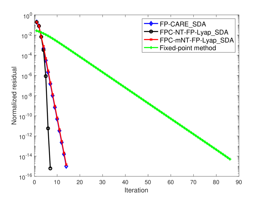
(ii). From the assertion (i), we have the sequence $\{X_{k}\}_{k=0}^{\infty}$ is monotonically nonincreasing and bounded below by $\widehat{X}$ . This implies that $\lim_{k\rightarrow\infty}X_{k}=\widehat{X}_{+}$ , where $\widehat{X}_{+}$ is a solution of SCARE (1.5). (iii). Since $A_{k}-G_{k}X_{k}$ is stable for each $k$ , by continuity $\sigma\left(A_{c}(\widehat{X}_{+})-G_{c}(\widehat{X}_{+})\widehat{X}_{+}\right)\subset\mathbb{C}_{-}\bigcup i\mathbb{R}$ . ∎

In practice, solving Lyapunov equation by Algorithm 2 outperforms solving CARE by SDA algorithm. However, it is difficult to find an initial matrix $X_{0}$ satisfying the conditions in Theorem 5.3 or Theorem 5.4. Moreover, comparing the Lyapunov equation in (4.5) with the CARE in (2.4), the CARE is more approximated the SCARE (1.5) than the Lyapunov equation. The convergence of FP-CARE_SDA algorithm will be better than that of mNT-FP-Lyap_SDA algorithm as shown in Figure 1.

To preserve the advantage and tackle the drawbacks of mNT-FP-Lyap_SDA algorithm, we proposed a practical algorithm that integrates FP-CARE_SDA and mNT-FP-Lyap_SDA algorithms. If we ignore the quadratic term $(X-X_{k})G_{k}(X-X_{k})$ in (5.2), then (5.2) is equal the CARE in (2.4). Assume that $X_{k}\geq 0$ in (5.2) is closed to the nonnegative solution of the SCARE (1.5). The norm of this quadratic term will be small, which means that FP-CARE_SDA and mNT-FP-Lyap_SDA algorithms will have the similar convergence. Furthermore, from Theorem 3.3, $\{X_{k}\}_{k=0}^{\infty}$ produced by FP-CARE_SDA with $X_{0}=0$ is monotonically nondecreasing and $\mathcal{R}(X_{k})\geq 0$ for all $k\geq 0$ . Therefore, we can use FP-CARE_SDA method in Algorithm 1 with $X_{0}=0$ to obtain $X_{k}$ , which is close enough to $\widehat{X}_{-}$ and $\mathcal{R}(X_{k})\geq 0$ . Based on Theorem 5.3, such $X_{k}$ can be used as an initial matrix of the mNT-FP-Lyap_SDA algorithm to improve the convergence of the mNT-FP-Lyap_SDA algorithm. We call this integrating method as the FPC-mNT-FP-Lyap_SDA method and state in Algorithm 6.

Algorithm 6 FPC-mNT-FP-Lyap_SDA method for solving SCARE (1.5)

A,Q\in\mathbb{R}^{n\times n}

B,L\in\mathbb{R}^{n\times m}

R=R^{\top}\in\mathbb{R}^{m\times m}

A_{0}^{i}\in\mathbb{R}^{n\times n}

B_{0}^{i}\in\mathbb{R}^{n\times m}

for

i=1,\ldots,r

, and a tolerance

\varepsilon

0: Solution

X

1: Set

k=0

and

\delta=\infty

2: Choose an initial

X_{0}^{\top}=X_{0}

3: Use FP-CARE_SDA algorithm (Algorithm 1) with initial

X_{0}

to compute an approximated

X_{k}

satisfied

\|X_{k}-X_{k-1}\|<0.01

4: Use mNT-FP-Lyap_SDA algorithm (Algorithm 4) with initial matrix

X_{k}

to solve SCARE (1.5).

6 Numerical experiments

In this section, we construct eight examples of SCAREs, in which $A$ , $B$ , $Q$ , $R$ come from the references and $A_{0}^{1},\ldots,A_{0}^{r}$ , $B_{0}^{1},\ldots,B_{0}^{r}$ are constructed in this paper. In the first four examples, we find an initial $X_{0}$ satisfying the conditions in Theorems 3.4 and 5.4 to numerically validate $\{X_{k}\}_{k=0}^{\infty}$ produced by FP-CARE_SDA and mNT-FP-Lyap_SDA algorithms to be monotonically nonincreasing and compare the convergence of the FP-CARE_SDA, NT-FP-Lyap_SDA and mNT-FP-Lyap_SDA algorithms. Such initial $X_{0}$ is difficult to find in Examples 5 - 8, then we use $X_{0}=0$ as the initial matrix. Theorem 3.3 shows $\{X_{k}\}_{k=0}^{\infty}$ to be monotonically nondecreasing for the FP-CARE_SDA algorithm. Numerical results show the failure of the convergence for the NT-FP-Lyap_SDA and mNT-FP-Lyap_SDA algorithms. However, the FPC-NT-FP-Lyap_SDA and FPC-mNT-FP-Lyap_SDA algorithms converge well to demonstrate the robustness of FP-CARE_SDA algorithm.

We use the normalized residual

\displaystyle\mbox{NRes}_{k}\equiv\frac{\|\mathcal{R}(X_{k})\|_{F}}{2\|AX_{k}\|_{F}+\|Q\|_{F}+\|\Pi_{11}(X_{k})\|_{F}+\|\mathcal{B}(X_{k})\|_{F}}

to measure the precision of the calculated solutions $X_{k}$ , where $\mathcal{B}(X)=(XB+L+\Pi_{12}(X))(R+\Pi_{22}(X))^{-1}(XB+L+\Pi_{12}(X))^{\top}$ . In Subsections 6.1 and 6.2, we demonstrate the convergence behaviors of $\mbox{NRes}_{k}$ for FP-CARE_SDA (Algorithm 1), NT-FP-Lyap_SDA (Algorithm 3), mNT-FP-Lyap_SDA (Algorithm 4), FPC-NT-FP-Lyap_SDA (Algorithm 5), FPC-mNT-FP-Lyap_SDA (Algorithm 6), and fixed-point iteration in (8.2) proposed by Guo and Liang [13]. The efficiency of these algorithms is demonstrated in Subsection 6.3.

All computations in this section are performed in MATLAB 2023a with an Apple M2 Pro CPU.

6.1 Numerical Validation of the convergence

Example 1.

Let

	$\displaystyle A$	$\displaystyle=\begin{bmatrix}0.9512&0\\ 0&0.9048\end{bmatrix},\quad B=\begin{bmatrix}4.8770&4.8770\\ -1.1895&3.5690\end{bmatrix},\quad Q=\begin{bmatrix}0.005&0\\ 0&0.020\end{bmatrix},\quad R=\begin{bmatrix}\frac{1}{3}&0\\ 0&3\end{bmatrix},\quad L=0,$
	$\displaystyle A_{0}^{1}$	$\displaystyle=\begin{bmatrix}-0.1&0.1\\ -0.2&0.2\end{bmatrix},\quad A_{0}^{2}=\begin{bmatrix}1&-0.1\\ 0.5&0\end{bmatrix},\quad A_{0}^{3}=\begin{bmatrix}0&-0.2\\ 0.2&0.5\end{bmatrix},$
	$\displaystyle B_{0}^{1}$	$\displaystyle=\begin{bmatrix}0&-0.1\\ 0.1&0\end{bmatrix},\quad B_{0}^{2}=\begin{bmatrix}0.5&1\\ -0.1&0.2\end{bmatrix},\quad B_{0}^{3}=\begin{bmatrix}1&-1\\ -0.2&1\end{bmatrix},$

where $A$ , $B$ , $Q$ and $R$ are given in Example 2.2 of [2].

Example 2.

Let

	$\displaystyle A$	$\displaystyle=\varepsilon\begin{bmatrix}\frac{7}{3}&\frac{2}{3}&0\\ \frac{2}{3}&2&-\frac{2}{3}\\ 0&-\frac{2}{3}&\frac{5}{3}\end{bmatrix},\quad B=\frac{1}{\sqrt{\varepsilon}}I_{3},\quad A_{0}^{1}=0.1\begin{bmatrix}0.1&-0.1&0.01\\ -0.2&0.1&-0.1\\ 0.05&-0.01&0.3\end{bmatrix},\quad R=I_{3},\quad L=0,$
	$\displaystyle Q$	$\displaystyle=\begin{bmatrix}(4\varepsilon+4+\varepsilon^{-1})/9&2(2\varepsilon-1-\varepsilon^{-1})/9&2(2-\varepsilon-\varepsilon^{-1})/9\\ 2(2\varepsilon-1-\varepsilon^{-1})/9&(1+4\varepsilon+4/\varepsilon)/9&2(-1-\varepsilon+2/\varepsilon)/9\\ 2(2-\varepsilon-\varepsilon^{-1})/9&2(-1-\varepsilon+2/\varepsilon)/9&(4+\varepsilon+4/\varepsilon)/9\end{bmatrix},\quad B_{0}^{1}=0.1\begin{bmatrix}0&0&0.2\\ 0.36&-0.6&0\\ 0&-0.95&-0.032\end{bmatrix}$

with $\varepsilon=0.01$ , where $A$ , $B$ , $Q$ and $R$ are given in Example 12 of [7].

Example 3.

Let

	$\displaystyle A$	$\displaystyle=\begin{bmatrix}0.9512&0\\ 0&0.9048\end{bmatrix},\quad B=\begin{bmatrix}4.8770&4.8770\\ -1.1895&3.5690\end{bmatrix},\quad Q=\begin{bmatrix}0.0028&-0.0013\\ -0.0013&0.0190\end{bmatrix},$
	$\displaystyle R$	$\displaystyle=\begin{bmatrix}1/3&0\\ 0&3\end{bmatrix},\quad A_{0}^{1}=6.5\begin{bmatrix}0.1&0.2\\ 0.2&0.1\end{bmatrix},\quad B_{0}^{1}=6.5I_{2},\quad L=0,$

modified in [27].

Example 4.

Let

	$\displaystyle A$	$\displaystyle=\begin{bmatrix}3-\varepsilon&1\\ 4&2-\varepsilon\end{bmatrix},\quad B=\begin{bmatrix}1\\ 1\end{bmatrix},\quad Q=\begin{bmatrix}4\varepsilon-11&2\varepsilon-5\\ 2\varepsilon-5&2\varepsilon-2\end{bmatrix},\quad A_{0}^{1}=\begin{bmatrix}0.1&-0.1\\ -0.2&0.1\end{bmatrix},$
	$\displaystyle B_{0}^{1}$	$\displaystyle=\begin{bmatrix}0.1\\ 0\end{bmatrix},\quad L=\begin{bmatrix}0\\ 0\end{bmatrix},\quad R=1,\ \mbox{ with }\ \varepsilon=5,$

where $A$ , $B$ , $Q$ and $R$ are given Example 11 of [7].

In Examples 1 - 4, we firstly take $X_{0}=0$ as the initial matrix for FP-CARE_SDA, NT-FP-Lyap_SDA and mNT-FP-Lyap_SDA algorithms. FP-CARE_SDA has a monotonically nondecreasing convergence as shown in Theorem 3.3. The numerical result shows that (i) the produced sequence converges to the solution $\widehat{X}_{-}\geq 0$ of the SCARE; (ii) NT-FP-Lyap_SDA and mNT-FP-Lyap_SDA algorithms fail to converge to $\widehat{X}_{-}$ .

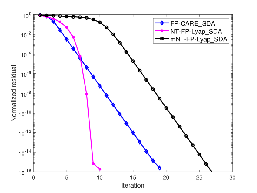
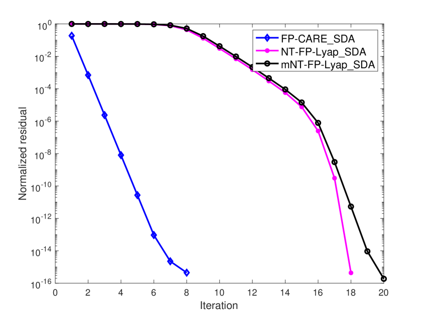
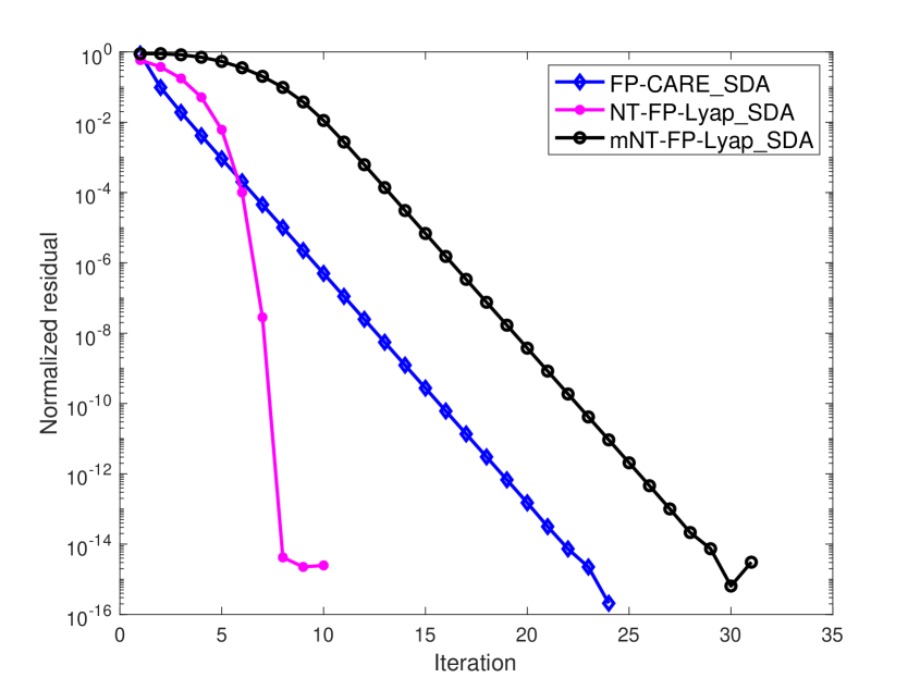
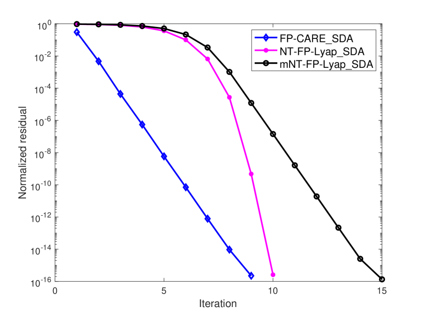
Next, we choose an initial $X_{0}$ with $\mathcal{R}(X_{0})\leq 0$ , $X_{0}\geq\widehat{X}$ , $A_{0}-G_{0}X_{0}$ being stable and $\rho(\mathcal{L}_{A_{X_{0}}}^{-1}\Pi_{X_{0}})<1$ so that $\{X_{k}\}_{k=0}^{\infty}$ produced by the FP-CARE_SDA, NT-FP-Lyap SDA and mNT-FP-Lyap SDA algorithms are monotonically nonincreasing and converge to the solution $\widehat{X}_{+}$ of the SCARE. Using the same initial $X_{0}$ for FP-CARE_SDA, NT-FP-Lyap_SDA and mNT-FP-Lyap_SDA algorithms, the normalized residual $\mbox{NRes}_{k}$ of the algorithms are shown in Figure 1. Numerical results show that $\widehat{X}_{+}=\widehat{X}{-}$ for these four examples.

The numerical results in Figure 1 show that the convergence of the FP-CARE_SDA algorithm is obviously better than that of the mNT-FP-Lyap_SDA algorithm. Furthermore, the normalized residuals at the first few iterations of the FP-CARE_SDA algorithm are less than those of the NT-FP-Lyap_SDA and mNT-FP-Lyap_SDA algorithms. These indicate that we can use a few iterations of FP-CARE_SDA algorithm to produce a good initial matrix $X_{0}$ for the NT-FP-Lyap_SDA and mNT-FP-Lyap_SDA algorithms, which are, called FPC-NT-FP-Lyap_SDA and FPC-mNT-FP-Lyap_SDA, respectively, used to improve the convergence and efficiency of the algorithms.

6.2 Robustness of FP-CARE_SDA algorithm

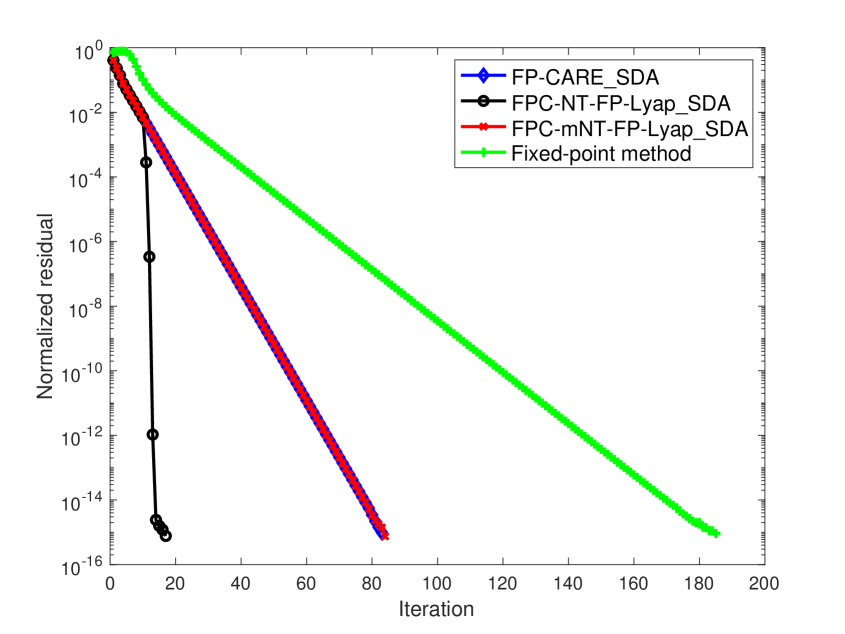
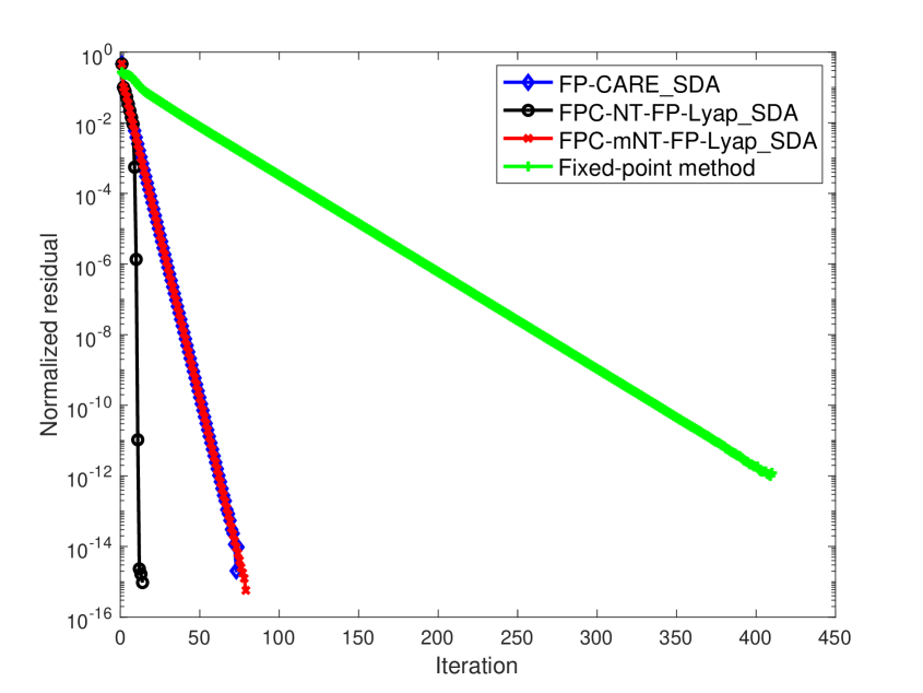
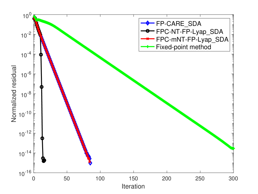
Due to the difficulty in selecting the initial matrix for Theorems 3.4 and 5.4, based on Theorem 3.3, we take $X_{0}=0$ as the initial matrix so that the FP-CARE_SDA algorithm has monotonically nondecreasing convergence. Numerical results show that the NT-FP-Lyap_SDA and mNT-FP-Lyap_SDA algorithms with $X_{0}=0$ fail to converge. In the following, we introduce four typical practical examples and discuss the convergence of the FPC-NT-FP-Lyap_SDA and FPC-mNT-FP-Lyap_SDA algorithms for these examples to demonstrate the robustness of FP-CARE_SDA algorithm.

Example 5.

The coefficient matrices, $A$ , $B$ , $Q$ , $R$ , and $L$ of a mathematical model of position and velocity controls for a string of high-speed vehicles [1] can be described as,

	$\displaystyle A$	$\displaystyle=\begin{bmatrix}C&D\\ &\ddots&\ddots\\ &&C&D\\ &&&C&-1\\ &&&&-1\end{bmatrix}\in\mathbb{R}^{(2m-1)\times(2m-1)},\quad C=\begin{bmatrix}-1&0\\ 1&0\end{bmatrix},\quad D=\begin{bmatrix}0&0\\ -1&0\end{bmatrix},$
	$\displaystyle B$	$\displaystyle=[b_{ij}]\in\mathbb{R}^{(2m-1)\times m},\quad b_{ij}=\begin{cases}1,&\mbox{ for }i=1,3,5,\ldots,2m-1,j=(i+1)/2,\\ 0,&\mbox{ otherwise},\end{cases}$
	$\displaystyle Q$	$\displaystyle=[q_{ij}]\in\mathbb{R}^{(2m-1)\times(2m-1)},\quad q_{ij}=\begin{cases}10,&\mbox{ for }i=2,4,6,\ldots,2m-1,\ j=i,\\ 0,&\mbox{ otherwise},\end{cases}$
	$\displaystyle R$	$\displaystyle=I_{m},\quad L=0_{(2m-1)\times m},$

where $m$ is the number of vehicles. Furthermore, the multiplicative white noises are

	$\displaystyle A_{0}^{i}$	$\displaystyle=0.1\times i\times\frac{\\|A\\|_{\infty}}{\\|\widehat{A}_{0}^{i}\\|_{\infty}}\widehat{A}_{0}^{i}\text{ with }\widehat{A}_{0}^{i}=\mbox{{wgn}}(2m-1,2m-1,8\times i),\mbox{ for }i=1,\ldots,5,$
	$\displaystyle B_{0}^{i}$	$\displaystyle=0.15\times i\times\frac{\\|B\\|_{\infty}}{\\|\widehat{B}_{0}^{i}\\|_{\infty}}\widehat{B}_{0}^{i}\text{ with }\widehat{B}_{0}^{i}=\mbox{{wgn}}(2m-1,m,3\times i),\mbox{ for }i=1,\ldots,5,$

where wgn is a MATLAB built-in function used to generate white Gaussian noise.

Example 6.

The differential SDRE with impact angle guidance strategies models the 3D missile/target interception engagement [20, 24]. The nonlinear dynamics can be expressed as in (1.1), where the system, the control and the white noise matrix are given by


$\displaystyle A(x)$	$\displaystyle=\begin{bmatrix}0&1&0&0&0\\ 0&\frac{-2\dot{r}}{r}&0&\frac{-1}{2}\dot{\psi}\sin(2x_{1}+2\theta_{f})&\frac{g_{1}}{z_{a}}\\ 0&0&0&1&0\\ 0&2\dot{\psi}\tan(x_{1}+\theta_{f})&0&\frac{-2\dot{r}}{r}&\frac{g_{2}}{z_{a}}\\ 0&0&0&0&-\eta\end{bmatrix}\ \ B(x)=\begin{bmatrix}0&0\\ \frac{-\cos\theta_{M}}{r}&0\\ 0&0\\ \frac{\sin\theta_{M}\sin\psi_{M}}{r\cos\theta}&\frac{-\cos\psi_{M}}{r\cos\theta}\\ 0&0\end{bmatrix},$
$\displaystyle A_{0}^{i}$	$\displaystyle=0.2\times i\times\frac{\\|A\\|_{\infty}}{\\|\widehat{A}_{0}^{i}\\|_{\infty}}\widehat{A}_{0}^{i}\ \text{ with }\ \widehat{A}_{0}^{i}=\mbox{{wgn}}(5,5,8\times i),\mbox{ for }i=1,\ldots,4,$	(6.1a)
$\displaystyle B_{0}^{i}$	$\displaystyle=0.1\times i\times\frac{\\|B\\|_{\infty}}{\\|\widehat{B}_{0}^{i}\\|_{\infty}}\widehat{B}_{0}^{i}\ \text{ with }\ \widehat{B}_{0}^{i}=\mbox{{wgn}}(5,2,3\times i),\mbox{ for }i=1,\ldots,4,$	(6.1b)

in which $r$ measures the distance between missile and target, $\{\psi,\theta\}$ (respective to $\{\psi_{M},\theta_{M}\}$ ) are the azimuth and elevation angles (respective to missile) corresponding to the initial frame (respective the line-of-sight (LOS) frame). Furthermore, the state vector $x=[x_{1},x_{2},x_{3},x_{4},x_{5}]^{\top}$ is defined by $x_{1}=\theta-\theta_{f}$ , $x_{2}=\dot{x}_{1}$ , $x_{3}=\psi-\psi_{f}$ , $x_{4}=\dot{x}_{3}$ with $\theta_{f}$ and $\psi_{f}$ being prescribed final angles, $x_{5}$ is a slow varying stable auxiliary variable governed by $\dot{x}_{5}=-\eta x_{5}$ , $\eta>0$ , $g_{1}$ and $g_{2}$ are highly nonlinear functions on $r$ , $\theta$ , $\psi$ , $\theta_{f}$ , $\psi_{f}$ , $\theta_{T}$ , $\psi_{T}$ , $a_{T}^{z}$ and $a_{T}^{y}$ (see [24] for details), where $\{\psi_{T},\theta_{T}\}$ are the azimuth and elevation angles of the target to the LOS frame, $a_{T}^{z}$ and $a_{T}^{y}$ are the lateral accelerations for the target, and $(u_{1},u_{2})=(a_{M}^{z},a_{M}^{y})$ is the control vector for the maneuverability of missile.

For a fixed state $x$ at the state-dependent technique of SDRE [20], the coefficient matrices of the SCARE (1.3) associated with the optimization problem (1.2) under the nonlinear dynamics for the missile/target engagement have the forms.

	$\displaystyle A$	$\displaystyle=\begin{bmatrix}0&1&0&0&0\\ 0&0.0696&0&-0.0307&-1.91\times 10^{-4}\\ 0&0&0&1&0\\ 0&0.123&0&0.0696&6.13\times 10^{-4}\\ 0&0&0&0&-0.1\end{bmatrix},\quad B=\begin{bmatrix}0&0\\ -9.13\times 10^{-5}&0\\ 0&0\\ 2.42\times 10^{-5}&-1.30\times 10^{-4}\\ 0&0\end{bmatrix},$
	$\displaystyle Q$	$\displaystyle={\rm diag}(1000,1000,1000,1000,0),\quad R=I_{2},\quad L=0,\quad A_{0}^{i}\text{ and }B_{0}^{i}\text{ are as in \eqref{eq6.1}.}$

Example 7.

[6] Finite-time SDRE of F16 aircraft flight control system [6] can be described as

	$\displaystyle\dot{\mathbf{x}}\equiv\begin{bmatrix}\dot{u}\\ \dot{v}\\ \dot{w}\\ \dot{p}\\ \dot{q}\\ \dot{r}\end{bmatrix}=$	$\displaystyle\begin{bmatrix}(g\sin\theta)/u&0&0&0&-w&v\\ (-g\sin\phi\cos\theta)/u&0&0&w&0&-u\\ (-g\cos\phi\cos\theta)/u&0&0&-v&u&0\\ 0&0&0&c_{1}q/2&(c_{1}p+c_{2}r)/2&c_{2}q/2\\ 0&0&0&c_{3}p+c_{4}r/2&0&c_{4}p/2-c_{3}r\\ 0&0&0&c_{5}q/2&(c_{5}p+c_{6}r)/2&c_{6}q/2\end{bmatrix}\begin{bmatrix}u\\ v\\ w\\ p\\ q\\ r\end{bmatrix}$
		$\displaystyle+\begin{bmatrix}1/m&0&0&0\\ 0&0&0&0\\ 0&0&0&0\\ 0&c_{lp}&0&c_{np}\\ c_{mq}Z_{TP}&0&c_{mq}&0\\ 0&c_{lr}&0&c_{nr}\end{bmatrix}\begin{bmatrix}F_{T}\\ L\\ M\\ N\end{bmatrix}\equiv A(\mathbf{x})\mathbf{x}+B(\mathbf{x})\mathbf{u},$

where $g$ is the gravity force, $m$ is the aircraft mass, $(u,v,w)$ , $(p,q,r)$ are the aircraft velocity and angular velocity vectors, respectively, for roll $\phi$ , pitch $\theta$ and yaw $\psi$ angles, $c$ ’s parameters are the suitable combinations of coefficients of the aircraft inertial matrix, the control vector $\mathbf{u}=[F_{T},L,M,N]^{\top}$ consists of the thrust, the resulted rolling, pitch and yawing moments from the layout of ailerons, elevators and rudders, $Z_{TP}$ is the position of the thrust point.

For a fixed state $\mathbf{x}$ , the coefficient matrices of the SCARE (1.3) with the optimization problem (1.4) has the forms

	$\displaystyle A$	$\displaystyle=\begin{bmatrix}3.958\times 10^{-5}&0&0&0&-5.866&-6.985\\ 2.116\times 10^{-4}&0&0&5.866&0&-84.66\\ -0.1158&0&0&6.985&84.66&0\\ 0&0&0&1.791\times 10^{-4}&4.303\times 10^{-3}&-5.006\times 10^{-3}\\ 0&0&0&-5.329\times 10^{-3}&0&-4.259\times 10^{-2}\\ 0&0&0&-4.769\times 10^{-3}&3.253\times 10^{-2}&-1.791\times 10^{-4}\end{bmatrix},$
	$\displaystyle B$	$\displaystyle=\begin{bmatrix}1.076\times 10^{-4}&0&0&0\\ 0&0&0&0\\ 0&0&0&0\\ 0&7.780\times 10^{-5}&0&7.780\times 10^{-5}\\ 3.964\times 10^{-6}&0&1.321\times 10^{-5}&0\\ 0&1.211\times 10^{-6}&0&1.171\times 10^{-5}\end{bmatrix},$
	$\displaystyle Q$	$\displaystyle=5000I_{6},\quad R=2\times 10^{-4}I_{4},\quad L=0,$
	$\displaystyle A_{0}^{i}$	$\displaystyle=0.012\times i\times\frac{\\|A\\|_{\infty}}{\\|\widehat{A}_{0}^{i}\\|_{\infty}}\widehat{A}_{0}^{i}\ \text{ with }\ \widehat{A}_{0}^{i}=\mbox{{wgn}}(6,6,100\times i),\mbox{ for }i=1,2,3,$
	$\displaystyle B_{0}^{i}$	$\displaystyle=0.012\times i\times\frac{\\|B\\|_{\infty}}{\\|\widehat{B}_{0}^{i}\\|_{\infty}}\widehat{B}_{0}^{i}\ \text{ with }\ \widehat{B}_{0}^{i}=\mbox{{wgn}}(6,4,40\times i),\mbox{ for }i=1,2,3.$

Example 8.

[5] The SDRE optimal control design for quadrotors for enhancing robustness against unmodeled disturbances [5] can be described as in (1.1) and (1.2) with $\mathbf{x}=[u,v,w,p,q,r,\phi,\theta,z_{a}]^{\top}$ , $\mathbf{e}=\mathbf{x}-\mathbf{x}_{f}$ ,

	$\displaystyle A(\mathbf{x})$	$\displaystyle=\begin{bmatrix}0&\frac{r}{2}&-\frac{q}{2}&0&-\frac{w}{2}&\frac{v}{2}&0&-\frac{g(\sin\theta)}{\theta}&0\\ -\frac{r}{2}&0&\frac{p}{2}&\frac{w}{2}&0&-\frac{u}{2}&\frac{g(1+\cos\theta)\sin\phi}{2\phi}&-\frac{g(1-\cos\theta)\sin\phi}{2\theta}&0\\ \frac{q}{2}&-\frac{p}{2}&0&-\frac{v}{2}&\frac{u}{2}&0&-\frac{2g}{\phi}\sin^{2}(\frac{\phi}{2})\cos^{2}(\frac{\theta}{2})&-\frac{2g}{\theta}\sin^{2}(\frac{\theta}{2})\cos^{2}(\frac{\phi}{2})&\frac{g}{z_{a}}\\ 0&0&0&0&\frac{c_{1}r}{2}&\frac{c_{1}q}{2}&0&0&0\\ 0&0&0&\frac{c_{2}r}{2}&0&\frac{c_{2}p}{2}&0&0&0\\ 0&0&0&\frac{c_{3}q}{2}&\frac{c_{3}p}{2}&0&0&0&0\\ 0&0&0&1&\frac{\sin\phi\tan\theta}{3}&\frac{\tan\theta(1+\cos\phi)}{3}&\frac{\alpha_{1}}{3\phi}&\frac{\alpha_{2}}{3\theta}&0\\ 0&0&0&0&\frac{1+\cos\phi}{2}&-\frac{\sin\phi}{2}&-\frac{\alpha_{3}}{2\phi}&0&0\\ 0&0&0&0&0&0&0&0&-\eta\end{bmatrix},$
	$\displaystyle B$	$\displaystyle=\begin{bmatrix}0&0&-\frac{1}{m}&0&0&0&0&0&0\\ 0&0&0&\frac{1}{I_{x}}&0&0&0&0&0\\ 0&0&0&0&\frac{1}{I_{y}}&0&0&0&0\\ 0&0&0&0&0&\frac{1}{I_{z}}&0&0&0\end{bmatrix}^{\top},$
	$\displaystyle Q$	$\displaystyle=\mbox{\rm diag}(2000,2000,3000,10,10,100,0,0,0),\ R=I_{4},\ L=0,$
	$\displaystyle A_{0}^{i}$	$\displaystyle=0.025\times i\times\frac{\\|A\\|_{\infty}}{\\|\widehat{A}_{0}^{i}\\|_{\infty}}\widehat{A}_{0}^{i}\ \text{ with }\ \widehat{A}_{0}^{i}=\mbox{{wgn}}(9,9,10\times i),\mbox{ for }i=1,2,3,$
	$\displaystyle B_{0}^{i}$	$\displaystyle=0.01\times i\times\frac{\\|B\\|_{\infty}}{\\|\widehat{B}_{0}^{i}\\|_{\infty}}\widehat{B}_{0}^{i}\ \text{ with }\ \widehat{B}_{0}^{i}=\mbox{{wgn}}(9,4,4\times i),\mbox{ for }i=1,2,3,$

where $\alpha_{1}=q\tan\theta\sin\phi-r\tan\theta+r\tan\theta\cos\phi$ , $\alpha_{2}=q\tan\theta\sin\phi+r\tan\theta\cos\phi$ , and $\alpha_{3}=q(1-\cos\phi)+r\sin\phi$ , $g$ is the gravity force, $m$ is the quadrotor mass, $(u,v,w)$ and $(p,q,r)$ are the velocity and the angular velocity on the body-fixed frame, respectively, for roll $\phi$ , pitch $\theta$ and yaw $\psi$ angles, $z_{a}$ is a slow varying stable auxiliary variable governed by $\dot{z}_{a}=-\eta z_{a}$ , $\eta>0$ , $c_{1}=\frac{I_{y}-I_{z}}{I_{x}}$ , $c_{2}=\frac{I_{z}-I_{x}}{I_{y}}$ , $c_{3}=\frac{I_{x}-I_{y}}{I_{z}}$ , and $I_{x}$ , $I_{y}$ , $I_{z}$ , are initial parameters.

For a fixed state $\mathbf{x}$ with $m=1$ , $I_{x}=I_{y}=0.01466$ , and $I_{z}=0.02848$ , the coefficient matrix $A\equiv A(\mathbf{x})$ has the form

\displaystyle A

\displaystyle=\begin{bmatrix}0&-8.208\mbox{e-}4&-1.047\mbox{e-}2&0&-1.234\mbox{e-}4&1.178&0&-9.8000&0\\ 8.208\mbox{e-}4&0&-1.603\mbox{e-}3&1.234\mbox{e-}4&0&2.203\mbox{e-}2&9.800&-5.436\mbox{e-}4&0\\ 1.047\mbox{e-}2&1.603\mbox{e-}3&0&-1.178&-2.203\mbox{e-}2&0&0&0&9.820\mbox{e-}1\\ 0&0&0&0&7.738\mbox{e-}4&-9.871\mbox{e-}3&0&0&0\\ 0&0&0&-7.738\mbox{e-}4&0&-1.511\mbox{e-}3&0&0&0\\ 0&0&0&0&0&0&0&0&0\\ 0&0&0&1.000&1.386\mbox{e-}8&2.499\mbox{e-}4&2.617\mbox{e-}6&-5.464\mbox{e-}4&0\\ 0&0&0&0&1.000&0&-9.650\mbox{e-}3&0&0\\ 0&0&0&0&0&0&0&0&-0.100\end{bmatrix}.

In Examples 5 - 8, we use $X_{0}=0$ as the initial matrix so that $\{X_{k}\}_{k=0}^{\infty}$ is monotonically non-decreasing for the FP-CARE_SDA algorithm. The associated convergence of $\mbox{NRes}_{k}$ for these examples is presented in Figure 2. Numerical results show that

•

It is well known that Newton’s method (NT-FP-Lyap_SDA algorithm) is highly dependent on the initial choice $X_{0}$ . When $X_{0}=0$ or $X_{0}\geq 0$ is randomly constructed, NT-FP-Lyap_SDA does not converge to $\widehat{X}\geq 0$ for these four examples. However, in Figure 2, after a few $m$ iterations of FP-CARE_SDA for obtaining $X_{m}$ with $\|X_{m}-X_{m-1}\|_{2}\leq 0.01$ , $X_{m}$ is closed to $\widehat{X}$ and Newton’s method with initial $X_{m}$ (i.e. FPC-NT-FP-Lyap_SDA algorithm) has quadratic convergence.
•

Numerical results in Figure 2 show that the fixed-point method, FP-CARE_SDA and FPC-mNT-FP-Lyap_SDA algorithms have linear convergence. But, the iteration number of the fixed-point method is obviously larger than that of the other methods. Comparing the results in Figure 2 with those in Figure 1, the iteration number of mNT-FP-Lyap_SDA algorithm in Figure 1 is obviously larger than that of FP-CARE_SDA algorithm. As shown in (5.2), the quadratic term $(X-X_{k})G_{k}(X-X_{k})$ is small when $X_{m}$ is used as an initial matrix of mNT-FP-Lyap_SDA algorithm. We can expect that the mNT-FP-Lyap_SDA algorithm with initial $X_{m}$ (i.e. FPC-mNT-FP-Lyap_SDA algorithm) has the same convergent behavior of the FP-CARE_SDA algorithm as presented in Figure 2. Without such initial $X_{m}$ (i.e., with $X_{0}=0$ or a randomly initial $X_{0}$ ), mNT-FP-Lyap_SDA algorithm will not converge for Examples 5 - 8. This demonstrates the importance and robustness of the FP-CARE_SDA algorithm.
•

For Examples 6 - 8, FPC-mNT-FP-Lyap_SDA algorithm produces monotonically non-decreasing sequences and has a linear convergence. The sequence produced by FPC-NT-FP-Lyap_SDA algorithm does not contain any monotonic property.

From the results in Figures 1 and 2, the FP-CARE_SDA algorithm has a linear convergence. Moreover, the FP-CARE_SDA algorithm also provides a good initial matrix for the NT-FP-Lyap_SDA algorithm and the modified Newton’s iteration in (4.5) so that the FPC-NT-FP-Lyap_SDA and FPC-mNT-FP-Lyap_SDA algorithms have quadratic and linear convergence, respectively. These two algorithms can not compute the solution $\widehat{X}$ without such an initial matrix. Therefore, our proposed FP-CARE_SDA algorithm is a reliable and robust algorithm.

6.3 Efficiency of algorithms

In each iteration of the FP-CARE_SDA (Algorithm 1), FPC-NT-FP-Lyap_SDA (Algorithm 5), and FPC-mNT-FP-Lyap_SDA (Algorithm 6), solving the CARE and Lyapunov equation are the most computationally intensive steps. To compare the efficiency of these methods, we first show the total numbers of solving CARE (2.4), Lyapunov equation (4.3)/(4.5), and fixed-point iteration (8.2) for each method in Table 1. The third and fifth columns show that we only need a few iterations of the FP-CARE_SDA algorithm to get a good initial matrix in FPC-NT-FP-Lyap_SDA and FPC-mNT-FP-Lyap_SDA algorithms.

	FP-CARE_SDA	FPC-NT-FP-Lyap_SDA		FPC-mNT-FP-Lyap_SDA		FP
	solving (2.4)	solving (2.4)	solving (4.3)	solving (2.4)	solving (4.5)	solving (8.2)
Exa. 5	14	3	16	3	11	86
Exa. 6	83	10	111	10	74	185
Exa. 7	74	8	114	8	71	410
Exa. 8	85	10	107	10	74	300

Table 1: Number of solving CARE (2.4), Lyapunov equation (4.3)/(4.5), and fixed-point (FP) iteration (8.2).

	CPU times (seconds)
	FP-CARE_SDA	FPC-NT-FP-Lyap_SDA	FPC-mNT-FP-Lyap_SDA	FP
Exa. 5	7.947e-1	8.112e-1	5.729e-1	5.790
Exa. 6	6.151e-3	4.632e-3	3.928e-3	9.634e-3
Exa. 7	5.527e-3	4.897e-3	3.816e-3	2.041e-2
Exa. 8	1.217e-2	7.759e-3	6.627e-3	3.804e-2

Table 2: CPU times for solving SCARE (1.5).

•

The fourth and sixth columns of Table 1 show that the FPC-NT-FP-Lyap_SDA algorithm still has a quadratic convergence, the convergence of the fixed-point iteration (4.3) for the FPC-NT-FP-Lyap_SDA algorithm is linear so that the total number of solving Lyapunov equations is larger than that for the FPC-mNT-FP-Lyap_SDA algorithm. As shown in Table 2, the performance of the FPC-mNT-FP-Lyap_SDA algorithm is better than that of the FPC-NT-FP-Lyap_SDA algorithm.
•

Sum of the numbers in the fifth and sixth columns of Table 1 is almost equal to the number in the second column. However, the computational cost for solving CARE (2.4) by SDA in [14] is larger than for solving Lyapunov equation (4.5) by L-SDA in Algorithm 2. This indicates that the FPC-mNT-FP-Lyap_SDA algorithm outperforms the FP-CARE_SDA algorithm as shown in the comparison of the CPU time in Table 2.
•

The dimension of the coefficient matrix for the linear system of the fixed-point iteration in (8.2) is $n(r+1)$ . Compared to the other three algorithms, in which matrix dimensions are $n$ , the fixed-point iteration needs more computational cost to solve the linear systems. On the other hand, as shown in Figures 1-2 and the last column in Table 1, the fixed-point iteration needs a large iteration number to get the solution. These lead to the performance of the fixed-point iteration being worse than that of the other three algorithms as shown in Table 2.

Summarized above results, we can see that the FPC-mNT-FP-Lyap_SDA algorithm outperforms the FP-CARE_SDA, FPC-NT-FP-Lyap_SDA algorithms, and fixed-point iteration.

7 Conclusions

We propose a reliable FP-CARE_SDA for solving the SCARE (1.3) and prove its monotonically non-decreasing convergence with $X_{0}=0$ , its monotonically non-increasing convergence with $\mathcal{R}(X_{0})\leq 0$ and $A_{0}-G_{0}X_{0}$ being stable. Furthermore, we propose the mNT-FP-Lyap_SDA algorithm to be used to accelerate the convergence with the FP-CARE_SDA as a robust initial step and prove its monotonically non-decreasing convergence under the assumption that the resulting $X_{k}\geq 0$ . Numerical experiments of real-world practical applications from the 3D missile/target engagement, the F16 aircraft flight control, and the quadrotor optimal control show the robustness of our proposed FPC-mNT-FP-Lyap_SDA algorithm.

8 Appendix

In [13], the authors proposed a fixed-point iteration to solve stochastic discrete-time algebraic Riccati equations (SDAREs) and proved the convergence of the fixed-point iteration. Moreover, the Möbius transformation is applied to transform the SCARE (1.5) into a SDARE so that the proposed fixed-point iteration can be applied to solve the associated solution $X$ . Now, we state the fixed-point iteration for solving SCARE. Let

\displaystyle\widehat{A}=A-BR^{-1}L^{\top},\quad\widehat{B}=BR^{-1/2},\quad\widehat{C}^{\top}\widehat{C}=Q-LR^{-1}L^{\top},

$\Pi$ and $\widehat{\Pi}\in\mathbb{R}^{n(r+1)\times n(r+1)}$ be the permutations satisfying

	$\displaystyle\Pi^{\top}(X\otimes I_{r})\Pi$	$\displaystyle=I_{r}\otimes X,$
	$\displaystyle\mbox{diag}\left(X,X\otimes I_{r}\right)$	$\displaystyle=\widehat{\Pi}^{\top}\left(X\otimes I_{r+1}\right)\widehat{\Pi},$

and

\displaystyle\mathcal{A}=\Pi\left(\begin{bmatrix}A_{0}^{1}\\ \vdots\\ A_{0}^{r}\end{bmatrix}-\begin{bmatrix}B_{0}^{1}\\ \vdots\\ B_{0}^{r}\end{bmatrix}R^{-1}L^{\top}\right),\quad\mathcal{B}=\Pi\begin{bmatrix}B_{0}^{1}\\ \vdots\\ B_{0}^{r}\end{bmatrix}R^{-/12}.

Give $\gamma>0$ so that $\widehat{A}_{\gamma}\equiv\widehat{A}-\gamma I_{n}$ is nonsingular. Define $Z_{\gamma}=\widehat{C}\widehat{A}_{\gamma}^{-1}\widehat{B}$ . By Möbius transformation, we have


$\displaystyle E_{\gamma}$	$\displaystyle=\widehat{\Pi}\begin{bmatrix}\widehat{A}_{\gamma}+2\gamma I_{n}+\widehat{B}Z_{\gamma}^{\top}\widehat{C}\\ \sqrt{2\gamma}(\mathcal{A}+\mathcal{B}Z_{\gamma}^{\top}\widehat{C})\end{bmatrix}(I_{n}+\widehat{A}_{\gamma}^{-1}\widehat{B}Z_{\gamma}^{\top}\widehat{C})^{-1}\widehat{A}_{\gamma}^{-1}\in\mathbb{R}^{n(r+1)\times n},$	(8.1a)
$\displaystyle H_{\gamma}$	$\displaystyle=2\gamma\widehat{A}_{\gamma}^{-\top}\widehat{C}^{\top}(I_{\ell}+Z_{\gamma}Z_{\gamma}^{\top})^{-1}\widehat{C}\widehat{A}_{\gamma}^{-1}\in\mathbb{R}^{n\times n},$	(8.1b)
$\displaystyle G_{\gamma}$	$\displaystyle=\widehat{\Pi}\begin{bmatrix}\sqrt{2\gamma}\widehat{A}_{\gamma}^{-1}\widehat{B}\\ \mathcal{A}\widehat{A}_{\gamma}^{-1}\widehat{B}-\mathcal{B}\end{bmatrix}(I_{m}+Z_{\gamma}^{\top}Z_{\gamma})^{-1}\begin{bmatrix}\sqrt{2\gamma}\widehat{A}_{\gamma}^{-1}\widehat{B}\\ \mathcal{A}\widehat{A}_{\gamma}^{-1}\widehat{B}-\mathcal{B}\end{bmatrix}^{\top}\widehat{\Pi}^{\top}\in\mathbb{R}^{n(r+1)\times n(r+1)}.$	(8.1c)

Then, the fixed-point iteration in [13] is given as

	$\displaystyle X_{1}$	$\displaystyle=H_{\gamma},$
	$\displaystyle X_{k+1}$	$\displaystyle=E_{\gamma}^{\top}(X_{k}\otimes I_{r+1})\left(I_{n(r+1)}+G_{\gamma}(X_{k}\otimes I_{r+1})\right)^{-1}E_{\gamma}+H_{\gamma}$		(8.2)

for $k=1,2,\ldots$ .

Each iteration in (8.2) only needs to compute $(X_{k}\otimes I_{r+1})\left(I_{n(r+1)}+G_{\gamma}(X_{k}\otimes I_{r+1})\right)^{-1}E_{\gamma}$ by the direct method. However, the dimension of the coefficient matrix is enlarged to $n(r+1)\times n(r+1)$ . It needs to have more and more computational cost as $r$ is large. On the other hand, the iteration can not preserve the symmetric property of the solution.

Acknowledgments

This work was partially supported by the National Science and Technology Council (NSTC), the National Center for Theoretical Sciences, and the Nanjing Center for Applied Mathematics. T.-M. Huang, Y.-C. Kuo, and W.-W. Lin were partially supported by NSTC 110-2115-M-003-012-MY3, 110-2115-M-390-002-MY3 and 112-2115-M-A49-010-, respectively.

References

[1] J. Abels and P. Benner. CAREX - a collection of benchmark examples for continuous-time algebraic Riccati equations. SLICOT Working Note 1999-16 (Version 2.0), December 1999. Available online at slicot.org/working-notes/.
[2] J. Abels and P. Benner. DAREX – a collection of benchmark examples for discrete-time algebraic Riccati equations. SLICOT Working Note 1999-14 (Version 2.0), December 1999. Available online at slicot.org/working-notes/.
[3] R. Babazadeh and R. Selmic. Distance-based multi-agent formation control with energy constraints using SDRE. IEEE Trans. Aerosp. Electron. Syst., 56(1):41–56, 2020.
[4] P. Benner and J. Heiland. Exponential stability and stabilization of extended linearizations via continuous updates of Riccati-based feedback. Int. J. Robust Nonlinear Control, 28(4):1218–1232, 2018.
[5] S.-W. Cheng and H.-A. Hung. Robust state-feedback ${H}_{\infty}$ control of quadrotor. International Automatic Control Conference, 2022.
[6] M. Chodnicki, P. Pietruszewski, M. Weso ̵lowski, and S. Stȩpień. Finite-time SDRE control of F16 aircraft dynamics. Arch. Control Sci., 32:557–576, 2022.
[7] E. K.-W. Chu, H.-Y. Fan, and W.-W. Lin. A structure-preserving doubling algorithm for continuous-time algebraic Riccati equations. Linear Algebra Appl., 396:55–80, 2005.
[8] E. K.-W. Chu, T. Li, W.-W. Lin, and C.-Y. Weng. A modified Newton’s method for rational Riccati equations arising in stochastic control. In 2011 International Conference on Communications, Computing and Control Applications (CCCA), pages 1–6, 2011.
[9] T. Çimen. Survey of state-dependent Riccati equation in nonlinear optimal feedback control synthesis. J. Guid. Control Dyn., 35(4):1025–1047, 2012.
[10] T. Damm and D. Hinrichsen. Newton’s method for a rational matrix equation occurring in stochastic control. Linear Algebra Appl., 332-334:81–109, 2001.
[11] V. Dragan, T. Morozan, and A.-M. Stoica. Mathematical Methods in Robust Control of Linear Stochastic Systems. Springer-Verlag, 2013.
[12] C.-H. Guo. Iterative solution of a matrix Riccati equation arising in stochastic control. In Linear Operators and Matrices, pages 209–221. Birkhäuser Basel, 2002.
[13] Z.-C. Guo and X. Liang. Stochastic algebraic Riccati equations are almost as easy as deterministic ones theoretically. arXiv, 2207.11220v3, 2023.
[14] T.-M. Huang, R.-C. Li, and W.-W. Lin. Structure-Preserving Doubling Algorithms for Nonlinear Matrix Equations. Society for Industrial and Applied Mathematics, Philadelphia, PA, 2018.
[15] I. G. Ivanov. Iterations for solving a rational Riccati equation arising in stochastic control. Comput. Math. Appl., 53:977–988, 2007.
[16] S. Kim and S. J. Kwon. Nonlinear optimal control design for underactuated two-wheeled inverted pendulum mobile platform. 22(6):2803–2808, 2017.
[17] P. Lancaster and L. Rodman. Existence and uniqueness theorems for the algebraic Riccati equation. Int. J. Control, 32:285–309, 1980.
[18] P. Lancaster and L. Rodman. Algebraic Riccati Equations. Oxford Science Publications. Oxford University Press, 1995.
[19] L.-G. Lin, Y.-W. Liang, and L.-J. Cheng. Control for a class of second-order systems via a state-dependent Riccati equation approach. SIAM J. Control Optim., 56(1):1–18, 2018.
[20] L.-G. Lin, R.-S. Wu, P.-K. Huang, M. Xin, C.-T. Wu, and W.-W. Lin. Fast SDDRE-based maneuvering-target interception at prespecified orientation. pages 1–8, 2023.
[21] L.-G. Lin and M. Xin. Alternative SDRE scheme for planar systems. IEEE Trans. Circuits Syst. II-Express Briefs, 66(6):998–1002, 2019.
[22] W.-W. Lin and S.-F. Xu. Convergence analysis of structure-preserving doubling algorithms for Riccati-type matrix equations. SIAM J. Matrix Anal. Appl., 28(1):26–39, 2006.
[23] Y. Meng, Q. Chen, X. Chu, and A. Rahmani. Maneuver guidance and formation maintenance for control of leaderless space-robot teams. IEEE Trans. Aerosp. Electron. Syst., 55(1):289–302, 2019.
[24] R. V. Nanavati, S. R. Kumar, and A. Maity. Spatial nonlinear guidance strategies for target interception at pre-specified orientation. Aerosp. Sci. Technol., 114:106735, 2021.
[25] S. R. Nekoo. Tutorial and review on the state-dependent Riccati equation. 8(2):109–166, 2019.
[26] V. Polito. Nonlinear business cycle and optimal policy: A VSTAR perspective. CESifo Working Paper Series, (8060):1–54, 2020.
[27] P. C.-Y. Weng and F. K.-H. Phoa. Perturbation analysis and condition numbers of rational Riccati equations. Ann. Math. Sci. Appl., 6:25–49, 2021.