On Potentials Integrated by the Nikiforov–Uvarov method

Lina Ellis Department of Mathematics and Statistics, Northern Arizona University, P. O. Box 5717, Flagstaff, AZ 86011, U.S.A. linabellis@gmail.com , Ikumi Ellis School of Mathematical and Statistical Sciences, Arizona State University, P. O. Box 871804, Tempe, AZ 85287-1804, U.S.A. irellis@asu.edu , Christoph Koutschan Johann Radon Institute for Computational and Applied Mathematics, Austrian Academy of Sciences, Altenberger Straße 69, 4040 Linz, Austria christoph.koutschan@ricam.oeaw.ac.at and Sergei K. Suslov School of Mathematical and Statistical Sciences, Arizona State University, P. O. Box 871804, Tempe, AZ 85287-1804, U.S.A. sergei@asu.edu

(Date: April 3, 2023)

Abstract.

We discuss basic potentials of the nonrelativistic and relativistic quantum mechanics that can be integrated in the Nikiforov and Uvarov paradigm with the aid of a computer algebra system. This approach may help the readers to study modern analytical methods of quantum physics.

2020 Mathematics Subject Classification:

Primary 81Q05, Secondary 33C45

C. K. was supported by the Austrian Science Fund (FWF): I6130-N

Building on ideas of de Broglie and Einstein, I tried to show that the ordinary differential equations of mechanics, which attempt to define the co-ordinates of a mechanical system as functions of the time, are no longer applicable for “small” systems; instead there must be introduced a certain partial differential equation, which defines a variable $\psi$ (“wave function”) as a function of the co-ordinates and the time.

Erwin Schrödinger [36]

1. Introduction

Discovery of the relativistic and nonrelativistic Schrödinger equations [33], [34], [35], [36], [37], [38] is discussed in [3] (see also the references therein). Invented about a century ago, the stationary Schrödinger equation turns out to have an enormously wide range of applications, from the quantum theory of atoms and molecules to solid state physics, quantum crystals, superfluidity, and superconductivity. Finding of the energy levels and the corresponding normalized wave functions of various systems is one of the basic problems of quantum physics. Only in a few elementary cases the exact solutions are known. They are usually investigated by different techniques. Nonetheless, those completely integrable problems are important in creation of mathematical models for complex quantum systems. Moreover, they may provide a useful testing ground for verification of numerical methods. A true story of calculations of the energy levels for the two-electron atoms [29] is presented in [20].

We assemble analytical solutions for a range of potentials in the nonrelativistic and relativistic quantum mechanics that are available in the literature. Data for most of the potentials that can be studied, in a unified way, by the so-called Nikiforov–Uvarov method [27] are collected, independently verified, and completed with the help of the Mathematica computer algebra system. Only bound states are discussed. On the contrary, in a traditional approach, for each of those problems one has to identify and factor out the singularities of the corresponding square integrable wave functions and find the remaining terminating power series expansions or use algebraic methods (see, for example, [4], [6], [7], [9], [10], [12], [17], [18], [23], [39], [40]). As a result, each of such problems has to be treated separately, which is not suitable for a unified computer algebra approach.

Our review article is organized as follows. In the next section, we introduce the basics of the Nikiforov–Uvarov approach and then, successively, apply it to the main problems of introductory quantum mechanics, such as harmonic oscillators, Bessel functions, Coulomb problems, Pöschl–Teller potential holes, Kratzer’s molecular potential, Hulthén potentials, and Morse potentials, in the forthcoming sections. All calculations are verified in a complementary Mathematica notebook that can serve both educational and research purposes. Appendices A and B contain, for the reader’s convenience, the data for classical orthogonal polynomials and a useful integral evaluation, respectively, in order to make our presentation as self-contained as possible. Appendix C describes the Mathematica notebook.

This review is written for those who study quantum mechanics and would like to see more details than in the classical textbooks by utilizing the advanced computer algebra system, Mathematica. It is motivated by an introductory course in mathematics of quantum mechanics which one of the authors (SKS) has been teaching at Arizona State University for more than two decades.

2. Summary of the Nikiforov–Uvarov approach

The generalized equation of the hypergeometric type

(2.1)

u^{\prime\prime}+\frac{\widetilde{\tau}(x)}{\sigma(x)}u^{\prime}+\frac{\widetilde{\sigma}(x)}{\sigma^{2}(x)}u=0

( $\sigma(x),$ $\widetilde{\sigma}(x)$ are polynomials of degrees at most $2$ and $\widetilde{\tau}(x)$ is a polynomial degree at most one) by the substitution

(2.2)

u=\varphi(x)y(x)

can be reduced to the form

(2.3)

\sigma(x)y^{\prime\prime}+\tau(x)y^{\prime}+\lambda y=0

if:

(2.4)

\frac{\varphi^{\prime}}{\varphi}=\frac{\pi(x)}{\sigma(x)},\qquad\pi(x)=\frac{1}{2}\left(\tau(x)-\widetilde{\tau}(x)\right)

(or, $\tau(x)=\widetilde{\tau}+2\pi,$ for later),

(2.5)

k=\lambda-\pi^{\prime}(x)\qquad(\text{or, }\lambda=k+\pi^{\prime}),

and

(2.6)

\pi(x)=\frac{\sigma^{\prime}-\widetilde{\tau}}{2}\pm\sqrt{\left(\frac{\sigma^{\prime}-\widetilde{\tau}}{2}\right)^{2}-\widetilde{\sigma}+k\sigma}

is a linear function. (Use the choice of the constant $k$ to complete the square under the radical sign; see [27] and our argument below for more details.)

In Nikiforov–Uvarov’s method, the energy levels can be obtained from the quantization rule:

(2.7)

\lambda+n\tau^{\prime}+\frac{1}{2}n(n-1)\sigma^{\prime\prime}=0\qquad(n=0,1,2,\dots)

and the corresponding square-integrable solutions are classical orthogonal polynomials, up to a factor. They can be found by the Rodrigues-type formula [27]:

(2.8)

y_{n}(x)=\dfrac{B_{n}}{\rho(x)}\left(\sigma^{n}(x)\rho(x)\right)^{(n)},\qquad(\sigma\rho)^{\prime}=\tau\rho,

where $B_{n}$ is a constant (see also [42] and Table 19). (The corresponding data for basic nonrelativistic and relativistic problems are presented in the Tables 1–18 below.)

Let us try to transform the differential equation (2.1) to the simplest form by the change of unknown function $u=\varphi(x)\,y$ with the help of some special choice of function $\varphi(x)$ .

Substituting $u=\varphi(x)\;y$ in (2.1) one gets

(2.9)

y^{\prime\prime}+\left(\frac{\widetilde{\tau}}{\sigma}+2\frac{\varphi^{\prime}}{\varphi}\right)y^{\prime}+\left(\frac{\widetilde{\sigma}}{\sigma^{2}}+\frac{\widetilde{\tau}}{\sigma}\frac{\varphi^{\prime}}{\varphi}+\frac{\varphi^{\prime\prime}}{\varphi}\right)y=0.

Equation (2.9) should not be more complicated than our original equation (2.1). Thus, it is natural to assume that the coefficient in front of $y^{\prime}$ has the form $\tau(x)/\sigma(x)$ , where $\tau(x)$ is a polynomial of degree at most one. This implies the following first-order differential equation

(2.10)

\frac{\varphi^{\prime}}{\varphi}=\frac{\pi(x)}{\sigma(x)}

for the function $\varphi(x)$ , where

(2.11)

\pi(x)=\frac{1}{2}\left(\tau(x)-\widetilde{\tau}(x)\right)

is a polynomial of degree at most one. As a result, equation (2.9) takes the form

(2.12)

y^{\prime\prime}+\frac{\tau(x)}{\sigma(x)}\;u^{\prime}+\frac{\overline{\sigma}(x)}{\sigma^{2}(x)}\;u=0,

where

(2.13)

\overline{\sigma}(x)=\widetilde{\sigma}(x)+\pi^{2}(x)+\pi(x)\left[\widetilde{\tau}(x)-\sigma^{\prime}(x)\right]+\pi^{\prime}(x)\sigma(x).

The functions $\tau(x)$ and $\overline{\sigma}(x)$ are polynomials of degrees at most one and two in $x$ , respectively. Therefore, equation (2.12) is an equation of the same type as our original equation (2.1).

By using a special choice of the polynomial $\pi(x)$ we can reduce (2.12) to the simplest form assuming that

(2.14)

\overline{\sigma}(x)=\lambda\;\sigma(x),

where $\lambda$ is some constant. Then equation (2.12) takes the form (2.3). We call equation (2.3) a differential equation of hypergeometric type and its solutions functions of hypergeometric type. In this context, it is natural to call equation (2.1) a generalized differential equation of hypergeometric type [27].

The condition (2.14) can be rewritten as

(2.15)

\pi^{2}+\left(\widetilde{\tau}-\sigma^{\prime}\right)\;\pi+\widetilde{\sigma}-k\sigma=0,

where

(2.16)

k=\lambda-\pi^{\prime}(z)

is a constant. Assuming that this constant is known, we can find $\pi(x)$ as a solution (2.6) of the quadratic equation (2.15). But $\pi(x)$ is a polynomial, therefore the second degree polynomial

(2.17)

p(x)=\left(\frac{\sigma^{\prime}(x)-\widetilde{\tau}(x)}{2}\right)^{2}-\widetilde{\sigma}(x)+k\sigma(x)

under the radical should be a square of a linear function and the discriminant of $p(x)$ should be zero. This condition gives an equation for the constant $k$ , which is, generally, a quadratic equation. Given $k$ as a solution of this equation, we find $\pi(x)$ by the quadratic formula (2.6), then $\tau(x)$ and $\lambda$ by (2.11) and (2.16). Finally, we find the function $\varphi(x)$ as a solution of (2.10). It is clear that the reduction of equation (2.1) to the simplest form (2.3) can be accomplished by a few different ways in accordance with different choices of the constant $k$ and different signs in (2.6) for $\pi(x)$ .

A closed form for the constant $k$ can be obtained as follows [3]. Let

(2.18)

p(x)={\left(\frac{\sigma^{\prime}-\widetilde{\tau}}{2}\right)^{2}-\widetilde{\sigma}+k\sigma}=q(x)+k\sigma(x)\/,

where

(2.19)

q(x)=\left(\frac{\sigma^{\prime}-\widetilde{\tau}}{2}\right)^{2}-\widetilde{\sigma}\/.

Completing the square, one gets

(2.20)

p(x)=\dfrac{p^{\prime\prime}}{2}\left(x+\frac{p^{\prime}(0)}{p^{\prime\prime}}\right)^{2}-\dfrac{\left(p^{\prime}(0)\right)^{2}-2p^{\prime\prime}p(0)}{2p^{\prime\prime}}\/,

where the last term must be eliminated:

(2.21)

{\left(p^{\prime}(0)\right)^{2}-2p^{\prime\prime}p(0)}=0\/.

Therefore,

(2.22)

\left(q^{\prime}(0)+k\sigma^{\prime}(0)\right)^{2}-2\left(q^{\prime\prime}+k\sigma^{\prime\prime}\right)\left(q(0)+k\sigma(0)\right)=0\/,

which results in the following quadratic equation:

(2.23)

ak^{2}+2bk+c=0.

Here,

(2.24)		$\displaystyle a=\left(\sigma^{\prime}(0)\right)^{2}-2\sigma^{\prime\prime}\sigma(0)\/,$
(2.25)		$\displaystyle b=q^{\prime}(0)\sigma^{\prime}(0)-\sigma^{\prime\prime}q(0)-\sigma(0)q^{\prime\prime}\/,$
(2.26)		$\displaystyle c=\left(q^{\prime}(0)\right)^{2}-2q^{\prime\prime}q(0)\/.$

Solutions are

(2.27)

k_{0}=-\dfrac{c}{2b},\qquad\text{if}\quad a=0

and

(2.28)

k_{1,2}=\dfrac{-b\pm\sqrt{d}}{a},\qquad\text{if}\quad a\neq 0\/.

Here,

(2.29)

d=b^{2}-ac=\left(\sigma(0)q^{\prime\prime}-\sigma^{\prime\prime}q(0)\right)^{2}-2\left(\sigma^{\prime}(0)q^{\prime\prime}-\sigma^{\prime\prime}q^{\prime}(0)\right)\left(\sigma(0)q^{\prime}(0)-\sigma^{\prime}(0)q(0)\right)\/.

As a result,

(2.30)

p(x)=\left[\dfrac{p^{\prime\prime}}{2}\left(x+\frac{p^{\prime}(0)}{p^{\prime\prime}}\right)^{2}\right]_{k=k_{0,1,2}}\/,

which allows evaluating the linear function $\pi(x)\/$ in the Nikiforov–Uvarov technique.

Examples, for the most integrable cases that are available in the literature, are presented in the Tables 1–18 below, where all these analytical arguments are implemented in a supplementary Mathematica notebook (Appendix C ).

3. Harmonic Oscillator

Let us consider the one-dimensional stationary Schrödinger equation for the harmonic oscillator:

(3.1)

-\frac{\hbar^{2}}{2m}\frac{d^{2}\psi}{dx^{2}}+\frac{1}{2}m\omega^{2}x^{2}\psi=E\psi

with the orthonormal real-valued wave function

(3.2)

\int_{-\infty}^{\infty}\psi^{2}(x)\ dx=1.

Introducing dimensionless variables

(3.3)

\psi(x)=u(\xi),\qquad x=\xi\sqrt{\frac{\hbar}{m\omega}},\quad E=\hbar\omega\varepsilon

one gets

(3.4)

u^{\prime\prime}+\left(2\varepsilon-\xi^{2}\right)u=0.

Here, $\sigma(\xi)=1,$ $\widetilde{\tau}(\xi)=0,$ and $\widetilde{\sigma}(\xi)=2\varepsilon-\xi^{2}.$ Therefore,

(3.5)

\pi(\xi)=\pm\sqrt{k-2\varepsilon+\xi^{2}}=\pm\xi,\qquad k=2\varepsilon.

We pick $\pi=-\xi,$ which gives a negative derivative for

(3.6)

\tau(\xi)=\widetilde{\tau}(\xi)+2\pi(\xi)=-2\xi.

Then

(3.7)

\frac{\varphi^{\prime}}{\varphi}=\frac{\pi(\xi)}{\sigma(\xi)}=-\xi,\qquad\varphi(\xi)=e^{-\xi^{2}/2}

and $\lambda=2\varepsilon-1,$ $\rho(\xi)=e^{-\xi^{2}}.$ The energy levels are $\varepsilon=\varepsilon_{n}=n+1/2,$ $(n=0,1,2,\dots)$ from (2.7). The eigenfunctions,

(3.8)

y_{n}(\xi)=B_{n}e^{\xi^{2}}\frac{d^{n}}{d\xi^{n}}\left(e^{-\xi^{2}}\right),

are, up to a normalization, the Hermite polynomials (Table 19).

As a result, the orthonormal wave functions are given by [34], [36], [23]

(3.9)

\psi(x)=\left(\frac{m\omega}{\pi\hbar}\right)^{1/4}\frac{1}{\sqrt{2^{n}n!}}\exp\left(-\frac{m\omega}{2\hbar}x^{2}\right)H_{n}\left(x\sqrt{\frac{m\omega}{\hbar}}\right),

corresponding to the discrete energy levels

(3.10)

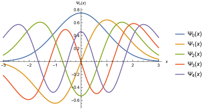
E_{n}=\hbar\omega\left(n+\frac{1}{2}\right)\qquad(n=0,1,2,\dots),

in Gaussian units; see also Figure 1 for graphs of the first five wave functions. (More general, “missing”, solutions of the time-dependent Schrödinger equation are discussed in [19], [21], and [24].)

Refer to caption — Figure 1. “The first five proper vibrations of the Planck oscillator according to undulatory mechanics. Outside the region $-3\leq x\leq 3$ , represented here, all five functions approach $x$ -axis in monotonic fashion.”— generated by Mathematica following the original Schrödinger article [36].

Table 1. Stationary Schrödinger equation for the harmonic potential

U(x)=\frac{1}{2}m\omega^{2}x^{2}.

$\sigma(\xi)$	$1$
$\widetilde{\sigma}(\xi)$	$2\varepsilon-\xi^{2}$
$\widetilde{\tau}(\xi)$	$0$
$k$	$2\varepsilon$
$\pi(\xi)$	$\pm\xi$
$\tau(\xi)=\widetilde{\tau}+2\pi\qquad$	$-2\xi$
$\lambda=k+\pi^{\prime}$	$2\varepsilon-1$
$\varphi(\xi)$	$e^{-\xi^{2}/2}$
$\rho(\xi)$	$e^{-\xi^{2}}$
$y_{n}(\xi)$	$C_{n}H_{n}(\xi)$
$C_{n}^{2}$	$\dfrac{1}{\sqrt{\pi}\,2^{n}n!}$

4. Bessel Functions

Let us also mention some solutions of the Bessel equation:

(4.1)

z^{2}u^{\prime\prime}+zu^{\prime}+\left(z^{2}-\nu^{2}\right)u=0.

With the aid of the change of the function $u=\varphi(z)y$ when $\varphi(z)=z^{\nu}e^{iz}$ this equation can be reduced to the hypergeometric form

(4.2)

zy^{\prime\prime}+(2iz+2\nu+1)y^{\prime}+i(2\nu+1)y=0

(Table 2) and one can obtain the Poisson integral representations for the Bessel functions of the first kind, $J_{\nu}(z)$ , and the Hankel functions of the first and second kind, $H_{\nu}^{(1)}(z)$ and $H_{\nu}^{(2)}(z)$ :

(4.3)		$\displaystyle J_{\nu}(z)$	$\displaystyle=\frac{(z/2)^{\nu}}{\sqrt{\pi}\,\Gamma(\nu+1/2)}\,\int_{-1}^{1}\,\left(1-t^{2}\right)^{\nu-1/2}\cos(zt)\,dt,$
(4.4)		$\displaystyle H_{\nu}^{(1,2)}(z)$	$\displaystyle=\sqrt{\frac{2}{\pi z}}\;\frac{e^{\pm i\left(z-\frac{\pi}{2}\nu-\frac{\pi}{4}\right)}}{\Gamma(\nu+1/2)}\,\int_{0}^{\infty}\,e^{-t}t^{\nu-1/2}\left(1\pm\frac{it}{2z}\right)^{\nu-1/2}dt,$

where $\text{Re}\,\nu>-1/2$ . It is then possible to deduce from these integral representations all the remaining properties of these functions. (For details, see [27] and [42] or [44] and [45]).

Table 2. Bessel’s equation.

$\sigma(z)$	$z$
$\widetilde{\sigma}(z)$	$z^{2}-\nu^{2}$
$\widetilde{\tau}(z)$	$1$
$k$	$\pm 2i\nu$
$\pi(z)$	$\pm\nu\pm iz$
$\tau(z)=\widetilde{\tau}+2\pi\qquad$	$1+2\nu+2iz$
$\lambda=k+\pi^{\prime}$	$i(2\nu+1)$
$\varphi(z)$	$z^{\pm\nu}e^{\pm iz}$
$\rho(z)$	$z^{2\nu}e^{2iz}$

5. Central Field: Spherical Harmonics

The stationary Schrödinger equation in the central field with the potential energy $U(r)$ is given by

(5.1)

\Delta\psi+\frac{2m}{\hbar^{2}}\left(E-U(r)\right)\psi=0.

The Laplace operator in the spherical coordinates $r,$ $\theta,$ $\varphi$ has the form [26], [27]:

(5.2)

\Delta=\Delta_{r}+\frac{1}{r^{2}}\Delta_{\omega}

with

(5.3)

\Delta_{r}=\frac{1}{r^{2}}\frac{\partial}{\partial r}\left(r^{2}\frac{\partial}{\partial r}\right),\quad\Delta_{\omega}=\frac{1}{\sin\theta}\frac{\partial}{\partial\theta}\left(\sin\theta\frac{\partial}{\partial\theta}\right)+\frac{1}{\sin^{2}\theta}\frac{\partial^{2}}{\partial\varphi^{2}}.

and separation of the variables $\psi=R(r)Y(\theta,\varphi)$ gives

(5.4)

\Delta_{\omega}Y(\theta,\varphi)+\mu Y(\theta,\varphi)=0,

(5.5)

\frac{1}{r^{2}}\frac{d}{dr}\left(r^{2}\frac{dR(r)}{dr}\right)+\left(\frac{2m}{\hbar^{2}}\left(E-U(r)\right)-\frac{\mu}{r^{2}}\right)R(r)=0.

Bounded single-valued solutions of equation (5.4) on the sphere $S^{2}$ exist only when $\mu=l(l+1)$ with $l=0,1,2,\dots\;.$ They are the spherical harmonics $Y=Y_{lm}(\theta,\varphi)$ .

Looking for solutions in the form $Y=e^{im\varphi}f(\theta)\/$ with $m=0,\pm 1,\pm 2,\dots$ one gets

(5.6)

\dfrac{1}{\sin\theta}\dfrac{d}{d\theta}\left(\sin\theta\,\dfrac{dg}{d\theta}\right)-\dfrac{m^{2}}{\sin^{2}\theta}\,g+\mu g=0.

The following change of variables $\xi=\cos\theta$ and $F(\xi)=f(\theta)$ results in the generalized equation of hypergeometric type:

(5.7)

\left(1-\xi^{2}\right)F^{\prime\prime}-2\xi F^{\prime}+\left(\mu-\dfrac{m^{2}}{1-\xi^{2}}\right)F=0,

with $\sigma(\xi)=1-\xi^{2},\,\widetilde{\tau}(\xi)=-2\xi\/$ and $\widetilde{\sigma}(\xi)=\mu\left(1-\xi^{2}\right)-m^{2}\/,$ which can be reduced to the simpler form by the standard substitution $F=\varphi\,y\/:$

(5.8)

\left(1-\xi^{2}\right)y^{\prime\prime}-2\left(|m|+1\right)\xi\,y^{\prime}+\left(\mu-|m|\left(|m|+1\right)\right)y=0

Indeed, by (2.6)

(5.9)

\pi(\xi)=\pm\sqrt{(\mu-k)\xi^{2}+k+m^{2}-\mu},

(5.10)

\pi(\xi)=\left\{\begin{array}[]{c}\pm|m|,\quad k=\mu\\ \pm|m|\,\xi,\quad k=\mu-m^{2}\end{array}\right.

where we should choose the case when the linear function $\tau=\widetilde{\tau}+2\pi$ will have a negative derivative and a zero on the interval $(-1,1)$ .

Then

(5.11)

\dfrac{\varphi^{\prime}}{\varphi}=\dfrac{-|m|\xi}{1-\xi^{2}},\qquad\ln\varphi=-|m|\int\frac{\xi\,d\xi}{1-\xi^{2}}=\dfrac{1}{2}\ln\left(1-\xi^{2}\right)

and

(5.12)

\varphi(\xi)=\left(1-\xi^{2}\right)^{|m|/2}=\left(\sin\theta\right)^{|m|}.

(see our complementary Mathematica notebook and Table 3 for further details of calculations).

The final result is given by

(5.13)

Y_{l\,m}(\theta,\varphi)=A_{m}\,\dfrac{e^{im\varphi}}{2^{|m|}\,l!}{\sqrt{\dfrac{2l+1}{4\pi}\,(l-m)!(l+m)!}}\;\left(\sin\theta\right)^{|m|}\,P_{l-|m|}^{(|m|,|m|)}(\cos\theta).

Here, $P_{n}^{(\alpha,\,\alpha)}(\xi)$ are the Jacobi polynomials (Table 19); $A_{m}=(-1)^{m},\,m\geq 0\/$ and $A_{m}=1,\,m<0\/.$ (See [26], [27], [43] for more details.)

Table 3. Equation for spherical harmonics.

$\sigma(\xi)$	$1-\xi^{2},\qquad\xi=\cos\theta,\quad 0\leq\theta\leq\pi$
$\widetilde{\sigma}(\xi)$	$\mu(1-\xi^{2})-m^{2}$
$\widetilde{\tau}(\xi)$	$-2\xi$
$k$	$\mu-m^{2}$
$\pi(\xi)$	$-\|m\|\xi$
$\tau(\xi)=\widetilde{\tau}+2\pi\qquad$	$-2\left(\|m\|+1\right)\xi$
$\lambda=k+\pi^{\prime}$	$\mu-\|m\|\left(\|m\|+1\right)$
$\varphi(\xi)$	$(1-\xi^{2})^{\|m\|/2}=(\sin\theta)^{\|m\|}$
$\rho(\xi)$	$(1-\xi^{2})^{\|m\|}$
$y_{n}(\xi)$	$N_{l\,m}\ P_{l-\|m\|}^{(\|m\|,\,\|m\|)}\left(\cos\theta\right),\quad n=l-\|m\|$
$N_{l\,m}$	$\dfrac{1}{2^{\|m\|}\,l!}{\sqrt{\dfrac{2l+1}{2}\,(l-m)!(l+m)!}}$

6. Nonrelativistic Coulomb Problem

In view of identity

(6.1)

\frac{1}{r^{2}}\frac{d}{dr}\left(r^{2}\frac{dR}{dr}\right)=\frac{1}{r}\frac{d^{2}}{dr^{2}}\left(rR\right),

the substitution $F(r)=rR(r)$ into (5.5) results in the standard radial equation

(6.2)

F^{\prime\prime}+\left[\frac{2m_{e}}{\hbar^{2}}\left(E-U(r)\right)-\frac{l(l+1)}{r^{2}}\right]F=0,\quad U(r)=-\frac{Ze^{2}}{r}

for the nonrelativistic Coulomb problem in spherical coordinates. In dimensionless units,

(6.3)

F(r)=u(x),\quad x=\frac{r}{a_{0}},\quad\varepsilon_{0}=\frac{E}{E_{0}}\quad\left(a_{0}=\frac{\hbar^{2}}{m_{e}e^{2}},\quad E_{0}=\frac{e^{2}}{a_{0}}\right)

the radial equation is a generalized equation of hypergeometric type,

(6.4)

u^{\prime\prime}+\left[2\left(\varepsilon_{0}+\frac{Z}{x}\right)-\frac{l(l+1)}{x^{2}}\right]u=0,

where

(6.5)

\sigma(x)=x,\qquad\widetilde{\tau}(x)=0,\qquad\widetilde{\sigma}(x)=2\varepsilon_{0}x^{2}+2Zx-l(l+1).

Therefore, one can utilize Nikiforov and Uvarov’s approach in order to determine the corresponding wave functions and discrete energy levels.

We transform (6.4) to the equation of hypergeometric type (2.3). The linear function $\pi(x)$ takes the form

(6.6)

\pi(x)=\frac{1}{2}\pm\sqrt{\frac{1}{4}-2\varepsilon_{0}x^{2}-2x+l(l+1)+kx},

(6.7)

\pi(x)=\frac{1}{2}\pm\left\{\begin{array}[]{c}\sqrt{-2\varepsilon_{0}}\ x+l+1/2,\quad k=2Z+(2l+1)\sqrt{-2\varepsilon_{0}}\\ \sqrt{-2\varepsilon_{0}}\ x-l-1/2,\quad k=2Z-(2l+1)\sqrt{-2\varepsilon_{0}}\end{array}\right.

where we should choose the case when the linear function $\tau=\widetilde{\tau}+2\pi$ will have a negative derivative and a zero on $(0,+\infty)$ :

\tau(x)=2\left(l+1-x\sqrt{-2\varepsilon_{0}}\right).

This choice corresponds to

\pi(x)=l+1-x\sqrt{-2\varepsilon_{0}},\quad\varphi(x)=x^{l+1}\exp\left(-x\sqrt{-2\varepsilon_{0}}\right)

and

\lambda=k+\pi^{\prime}=2\left[Z-(l+1)\sqrt{-2\varepsilon_{0}}\ \right].

The energy values are given by (2.7):

(6.8)

\varepsilon_{0}=\frac{E}{E_{0}}=-\frac{Z^{2}}{2\left(n_{r}+l+1\right)^{2}},\qquad E_{0}=\frac{e^{2}}{a_{0}}.

Here, $n=n_{r}+l+1$ is known as the principal quantum number.

In order to use the Rodrigues formula, one finds

\frac{\rho^{\prime}}{\rho}=\frac{\tau-\sigma^{\prime}}{\sigma}=\frac{2l+1}{x}-\frac{2Z}{n},

\rho(x)=x^{2l+1}\exp\left(-\frac{2Z}{n}x\right),\qquad x=\frac{r}{a_{0}}.

Therefore,

(6.9)

y_{n_{r}}(x)=\frac{B_{n_{r}}}{x^{2l+1}e^{-\eta}}\frac{d^{n_{r}}}{dx^{n_{r}}}\left(x^{n_{r}+2l+1}e^{-\eta}\right)=L_{n_{r}}^{2l+1}(\eta),

where

\eta=\frac{2Z}{n}x=\frac{2Z}{n}\left(\frac{r}{a_{0}}\right)=2x\sqrt{-2\varepsilon_{0}},

and, up to a constant,

(6.10)

F(r)=rR(r)=C_{nl}\ \eta^{l+1}e^{-\eta/2}L_{n_{r}}^{2l+1}(\eta).

In view of the normalization condition

1=\int_{0}^{\infty}F^{2}\ dr=C_{nl}^{2}\left(\frac{na_{0}}{2Z}\right)\int_{0}^{\infty}\eta^{2l+2}e^{-\eta}\left[L_{n_{r}}^{2l+1}(\eta)\right]^{2}\ d\eta,

the three-term recurrence relation

\eta L_{n}^{\alpha}=-(n+1)L_{n+1}^{\alpha}+(\alpha+2n+1)L_{n}^{\alpha}-(\alpha+n)L_{n-1}^{\alpha},

and the orthogonality property of the Laguerre polynomials (Table 19), one gets

(6.11)

C_{nl}^{2}=\frac{Z}{a_{0}n^{2}}\frac{(n-l-1)!}{(n+l)!}.

More details can be found in [27] and [42]. (See also Appendices A and B.)

As a result, the nonrelativistic Coulomb wave functions obtained by the method of separation of the variables in spherical coordinates, see above, are

(6.12)

\psi=\psi_{nlm}({\bf r})=R_{nl}(r)\ Y_{lm}(\theta,\varphi),

where $Y_{lm}(\theta,\varphi)$ are the spherical harmonics, the radial functions $R_{nl}(r)$ are given in terms of the Laguerre polynomials (Table 19) [4], [10], [23], [27], [39] :

(6.13)

R(r)=R_{nl}(r)=\frac{2}{n^{2}}\left(\frac{Z}{a_{0}}\right)^{3/2}\sqrt{\frac{(n-l-1)!}{(n+l)!}}\ e^{-\eta/2}\eta^{l}\ L_{n-l-1}^{2l+1}(\eta)

with

(6.14)

\eta=\frac{2Z}{n}\left(\frac{r}{a_{0}}\right),\qquad a_{0}=\dfrac{\hbar^{2}}{{m_{e}}e^{2}}

and the normalization is

(6.15)

\int_{0}^{\infty}R_{nl}^{2}(r)r^{2}\ dr=1.

Here $n=1,2,3,\dots$ is the principal quantum number of the hydrogen-like atom in the nonrelativistic Schrödinger theory; $l=0,1,\dots,n-1$ and $m=-l,-l+1,\dots,l-1,l$ are the quantum numbers of the angular momentum and its projection on the $z$ -axis, respectively. The corresponding discrete energy levels in the cgs units are given by Bohr’s formula [33]:

(6.16)

E=E_{n}=-\frac{{m_{e}}Z^{2}e^{4}}{2\hbar^{2}n^{2}},

where $n=1,2,3,\dots$ is the principal quantum number; they do not depend on the quantum number of the orbital angular momenta $l\/.$

Table 4. The Schrödinger equation for the Coulomb potential

U(r)=-Ze^{2}/r

. Dimensionless quantities:

r=a_{0}x

a_{0}=\hbar^{2}/(m_{e}e^{2})\simeq 0.5\cdot 10^{-8}\;\text{cm}

E_{0}=e^{2}/a_{0}

R(r)=F(x)=u(x)/x

$\sigma(x)$	$x$
$\widetilde{\sigma}(x)$	$2\varepsilon_{0}\;x^{2}+2Z\;x-l(l+1)\/,\quad{\varepsilon_{0}=E/E_{0}}$
$\widetilde{\tau}(x)$	$0$
$k$	$2Z-(2l+1)\sqrt{-2\varepsilon_{0}\/}$
$\pi(x)$	$l+1-\sqrt{-2\varepsilon_{0}}\;x$
$\tau(x)=\widetilde{\tau}+2\pi\qquad$	$2\left(l+1-\sqrt{-2\varepsilon_{0}}\;x\right)$
$\lambda=k+\pi^{\prime}$	$2\left(Z-(l+1)\sqrt{-2\varepsilon_{0}}\right)$
$\varphi(x)$	$x^{l+1}e^{-x\sqrt{-2\varepsilon_{0}}}$
$\rho(x)$	$x^{2l+1}e^{-(2Z\ x)/n},\quad x=r/a_{0}$
$y_{n_{r}}(x)$	$C_{n_{r}}L_{n_{r}}^{2l+1}(\eta),\quad\eta=\dfrac{2Z}{n}x=\dfrac{2Z}{n}\left(\dfrac{r}{a_{0}}\right)$
$C_{n_{r}}^{2}$	$\dfrac{Z}{a_{0}n^{2}}\dfrac{(n-l-1)!}{(n+l)!},\quad n_{r}=n-l-1$

Remark. In the original Nikiforov–Uvarov approach, the variable coefficients $\sigma(x)$ and $\tau(x)$ in (2.3) should not depend on the eigenvalue $\lambda$ . Here, we obtain

(6.17)

xy^{\prime\prime}+2\left(l+1-x\sqrt{-2\varepsilon_{0}}\right)y^{\prime}+2\left(Z-(l+1)\sqrt{-2\varepsilon_{0}}\right)y=0\/.

Nonetheless, the change of variables $y(x)=Y(\eta)$ with $\eta=2x\sqrt{-2\varepsilon_{0}}$ results in

(6.18)

\eta Y^{\prime\prime}+\left(2l+2-\eta\right)Y^{\prime}+\left(\dfrac{Z}{\sqrt{-2\varepsilon_{0}}}-l-1\right)Y=0\/.

Thus the Nikiforov–Uvarov method can be applied and the uniqueness of square integrable solutions holds.

In a similar fashion, one can consider solution of the Kepler problem in the so-called parabolic coordinates, which is important in the theory of Stark effect [35], [23].

7. Relativistic Schrödinger Equation

The stationary relativistic Schrödinger equation has the form [3], [7], [17], [39]:

(7.1)

\left(E+\frac{Ze^{2}}{r}\right)^{2}\chi=\left(-\hbar^{2}c^{2}\Delta+m^{2}c^{4}\right)\chi.

We separate the variables in spherical coordinates, $\chi(r,\theta,\varphi)=R(r)Y_{lm}(\theta,\varphi),$ where $Y_{lm}(\theta,\varphi)$ are the spherical harmonics with familiar properties [43]. As a result,

(7.2)

\frac{1}{r^{2}}\frac{d}{dr}\left(r^{2}\frac{dR}{dr}\right)+\left[\frac{\left(E+Ze^{2}/r\right)^{2}-m^{2}c^{4}}{\hbar^{2}c^{2}}-\frac{l(l+1)}{r^{2}}\right]R=0\qquad(l=0,1,2,\dots).

In the dimensionless quantities,

(7.3)

\varepsilon=\frac{E}{mc^{2}},\qquad x=\beta r=\frac{mc}{\hbar}r,\qquad\mu=\frac{Ze^{2}}{\hbar c},

for the new radial function,

(7.4)

R(r)=F(x)=\frac{u(x)}{x},

one gets

(7.5)

\frac{1}{x^{2}}\frac{d}{dx}\left(x^{2}\frac{dF}{dx}\right)+\left[\left(\varepsilon+\frac{\mu}{x}\right)^{2}-1-\frac{l(l+1)}{x^{2}}\right]F=0.

Given the identity $(x^{2}F^{\prime})^{\prime}=x(xF)^{\prime\prime}$ , we obtain

(7.6)

u^{\prime\prime}+\left[\left(\varepsilon+\frac{\mu}{x}\right)^{2}-1-\frac{l(l+1)}{x^{2}}\right]u=0.

This is the generalized equation of hypergeometric form (2.1), when

(7.7)

\sigma(x)=x,\qquad\widetilde{\tau}(x)\equiv 0,\qquad\widetilde{\sigma}(x)=\left(\varepsilon^{2}-1\right)x^{2}+2\mu\varepsilon x+\mu^{2}-l(l+1)

The normalization condition takes the form:

(7.8)

\int_{0}^{\infty}R^{2}(r)r^{2}\ dr=1,\qquad\text{or\quad}\int_{0}^{\infty}u^{2}(x)\;dx=\beta^{3},\quad\beta=\frac{mc}{\hbar}.

Here, $u=\varphi\,y\/.$ For further computational details, see our supplementary Mathematica notebook, as well as Refs. [3] and [27]. Final results are presented in Table 5.

In particular, one gets Schrödinger’s fine structure formula (for a charged spin-zero particle in the Coulomb field):

(7.9)

E=E_{n_{r}}=\frac{mc^{2}}{\sqrt{1+\left(\dfrac{\mu}{n_{r}+\nu+1}\right)^{2}}}\qquad\left(n=n_{r}=0,1,2,\dots\right).

Here,

(7.10)

\mu=\frac{Ze^{2}}{\hbar c},\qquad\nu=-\frac{1}{2}+\sqrt{\left(l+\frac{1}{2}\right)^{2}-\mu^{2}}.

The corresponding eigenfunctions are given by the Rodrigues-type formula

(7.11)

y_{n}(x)=\frac{B_{n}}{x^{2\nu+1}e^{-2ax}}\frac{d^{n}}{dx^{n}}\left(x^{n+2\nu+1}e^{-2ax}\right)=C_{n}L_{n}^{2\nu+1}(2ax).

Up to a constant, they are Laguerre polynomials (Table 19). In view of the normalization condition (7.8):

	$\displaystyle\beta^{3}$	$\displaystyle=\int_{0}^{\infty}u^{2}(x)\;dx=C_{n}^{2}\int_{0}^{\infty}\left[\varphi(x)L_{n}^{2\nu+1}(2ax)\right]^{2}\ dx$
(7.12)			$\displaystyle=\frac{C_{n}^{2}}{(2a)^{2\nu+3}}\int_{0}^{\infty}e^{-\xi}\,\xi^{2\nu+2}\left(L_{n}^{2\nu+1}(\xi)\right)^{2}\ d\xi,\quad\xi=2ax.$

The corresponding integral is given by (see [41], [42], and Appendix B):

(7.13)

I_{1}=J^{\alpha\alpha}_{nn1}=\int_{0}^{\infty}e^{-x}x^{\alpha+1}\left(L_{n}^{\alpha}(x)\right)^{2}\ dx=(\alpha+2n+1)\frac{\Gamma(\alpha+n+1)}{n!}.

As a result,

(7.14)

C_{n}=2(a\beta)^{3/2}(2a)^{\nu}\sqrt{\frac{n!}{\Gamma(2\nu+n+2)}}.

The normalized radial eigenfunctions, corresponding to the relativistic energy levels (7.9), are explicitly given by

(7.15)

R(r)=R_{n_{r}}(r)=2(a\beta)^{3/2}\sqrt{\frac{n_{r}!}{\Gamma(2\nu+n_{r}+2)}}\;\xi^{\nu}e^{-\xi/2}\;L_{n_{r}}^{2\nu+1}(\xi),

where

(7.16)

\xi=2ax=2a\beta r=2\sqrt{1-\varepsilon^{2}}\,\frac{mc}{\hbar}\,r.

(More details can be found in [3], [7], [39].)

Let us analyze a nonrelativistic limit of Schrödinger’s fine structure formula (7.9)–(7.10):

	$\displaystyle\varepsilon_{\text{Schr\"{o}dinger}}=\frac{E_{n_{r},\,l}}{mc^{2}}$	$\displaystyle=\frac{1}{\sqrt{1+\dfrac{\mu^{2}}{\left(n_{r}+\frac{1}{2}+\sqrt{\left(l+\frac{1}{2}\right)^{2}-\mu^{2}}\right)^{2}}}}$
(7.17)			$\displaystyle=1-\frac{\mu^{2}}{2n^{2}}-\frac{\mu^{4}}{2n^{4}}\left(\frac{n}{l+1/2}-\frac{3}{4}\right)+\text{O}(\mu^{6}),\quad\mu\rightarrow 0,$

which can be derived by a direct Taylor expansion and/or verified by a computer algebra system (see our supplementary Mathematica notebook). Here, $n=n_{r}+l+1$ is the corresponding nonrelativistic principal quantum number. The first term in this expansion is simply the rest mass energy $E_{0}=mc^{2}$ of the charged spin-zero particle, the second term coincides with the energy eigenvalue in the nonrelativistic Schrödinger theory and the third term gives the so-called fine structure of the energy levels, which removes the degeneracy between states of the same $n$ and different $l\/.$

Table 5. Relativistic Schrödinger equation for Coulomb potential

U(r)=-Ze^{2}/r

. Dimensionless quantities:

\varepsilon=E/(mc^{2})

x=\beta r=(mc/\hbar)r

\mu=Ze^{2}/(\hbar c)

R(r)=F(x)=u(x)/x

$\sigma(x)$	$x$
$\widetilde{\sigma}(x)$	$\left(\varepsilon^{2}-1\right)\;x^{2}+2\mu\varepsilon\;x+\mu^{2}-l(l+1)$
$\widetilde{\tau}(x)$	$0$
$k$	$2\mu\varepsilon-(2\nu+1)\sqrt{1-\varepsilon^{2}},\quad\nu=-\dfrac{1}{2}+\sqrt{\left(l+\dfrac{1}{2}\right)^{2}-\mu^{2}}$
$\pi(x)$	$\nu+1-a\;x,\qquad a=\sqrt{1-\varepsilon^{2}}$
$\tau(x)=\widetilde{\tau}+2\pi$	$2\left(\nu+1-a\;x\right),\quad\tau^{\prime}<0$
$\lambda=k+\pi^{\prime}$	$2\left(\mu\varepsilon-(\nu+1)a\right)$
$\varphi(x)$	$x^{\nu+1}e^{-a\ x}$
$\rho(x)$	$x^{2\nu+1}e^{-2a\ x}$
$y_{n_{r}}(x)$	$C_{n_{r}}L_{n_{r}}^{2\nu+1}(\xi),\quad\xi=2ax=2a\beta r=2\sqrt{1-\varepsilon^{2}}\dfrac{mc}{\hbar}r$
$C_{n_{r}}$	$2(a\beta)^{3/2}(2a)^{\nu}\sqrt{\dfrac{n_{r}!}{(\nu+n_{r}+1)\Gamma(2\nu+n_{r}+2)}}$

Once again, our equation,

(7.18)

xy^{\prime\prime}+2(\nu+1-ax)y^{\prime}+2\left(\mu\varepsilon-(\nu+1)a\right)y=0\/,

by the change of variables $y(x)=Y(\xi)$ with $\xi=2ax$ can be transformed into the required form:

(7.19)

\xi Y^{\prime\prime}+(2\nu+2-\xi)Y^{\prime}\left(\dfrac{\mu\varepsilon}{\sqrt{1-\varepsilon^{2}}}-\nu-1\right)Y=0\/.

Therefore, the set of the square integrable solutions above is unique.

8. Relativistic Coulomb Problem: Dirac Equation

8.1. System of radial equations

The radial Dirac equations are derived in Refs. [27], [41], and [42] by separation of variables in spherical coordinates (see also [4], [7], [10], [12], and [17]). Then the radial functions $F(r)$ and $G(r)$ satisfy the system of two first-order ordinary differential equations

(8.1)		$\displaystyle\dfrac{dF}{dr}+\frac{1+\kappa}{r}\ F$	$\displaystyle=\dfrac{mc^{2}+E-U(r)}{\hbar c}\ G,$
(8.2)		$\displaystyle\dfrac{dG}{dr}+\frac{1-\kappa}{r}\ G$	$\displaystyle=\dfrac{mc^{2}-E+U(r)}{\hbar c}\ F,$

where $\kappa=\kappa_{\pm}=\pm(j+1/2)=\pm 1,\pm 2,\pm 3,\dots$ respectively. For the relativistic Coulomb problem, when $U=-Ze^{2}/r,$ we introduce the dimensionless quantities

(8.3)

\varepsilon=\frac{E}{mc^{2}},\qquad x=\beta r=\frac{mc}{\hbar}r,\qquad\mu=\frac{Ze^{2}}{\hbar c}

and change the variable in radial functions

(8.4)

f(x)=F(r),\qquad g(x)=G(r).

The Dirac radial system becomes

(8.5)		$\displaystyle\dfrac{df}{dx}+\frac{1+\kappa}{x}\ f$	$\displaystyle=\left(1+\varepsilon+\frac{\mu}{x}\right)g,$
(8.6)		$\displaystyle\dfrac{dg}{dx}+\frac{1-\kappa}{x}\ g$	$\displaystyle=\left(1-\varepsilon-\frac{\mu}{x}\right)f.$

(One can show later that in the nonrelativistic limit, $c\rightarrow\infty\/,$ the following estimate holds: $\left|f(x)\right|\gg{\left|g(x)\right|}\/;$ see, for example, Refs. [27], [41], and [42] for more details.)

8.2. Decoupling of the radial system

We follow [27] with somewhat different details. Let us rewrite the system (8.5)–(8.6) in a matrix form. If

(8.7)

u=\begin{pmatrix}u_{1}\vskip 6.0pt plus 2.0pt minus 2.0pt\\ u_{2}\end{pmatrix}=\begin{pmatrix}xf(x)\vskip 6.0pt plus 2.0pt minus 2.0pt\\ xg(x)\end{pmatrix},\qquad u^{\prime}=\begin{pmatrix}u_{1}^{\prime}\vskip 6.0pt plus 2.0pt minus 2.0pt\\ u_{2}^{\prime}\end{pmatrix}.

Then

(8.8)

u^{\prime}=Au,

where

(8.9)

A=\begin{pmatrix}a_{11}&a_{12}\vskip 6.0pt plus 2.0pt minus 2.0pt\\ a_{21}&a_{22}\end{pmatrix}=\begin{pmatrix}-\dfrac{\kappa}{x}&1+\varepsilon+\dfrac{\mu}{x}\;\\[6.0pt] 1-\varepsilon-\dfrac{\mu}{x}&\dfrac{\kappa}{x}\end{pmatrix}.

To find $u_{1}(x)$ , we eliminate $u_{2}(x)$ from the system (8.8), obtaining a second-order differential equation

(8.10)		$\displaystyle u_{1}^{\prime\prime}-\left(a_{11}+a_{22}+\dfrac{a_{12}^{\prime}}{a_{12}}\right)u_{1}^{\prime}$
	$\displaystyle\qquad+\left(a_{11}a_{22}-a_{12}a_{21}-a_{11}^{\prime}+\dfrac{a_{12}^{\prime}}{a_{12}}\;a_{11}\right)u_{1}=0.$

Similarly, eliminating $u_{1}(x)$ , one gets an equation for $u_{2}(x)$ :

(8.11)		$\displaystyle u_{2}^{\prime\prime}-\left(a_{11}+a_{22}+\dfrac{a_{21}^{\prime}}{a_{21}}\right)u_{2}^{\prime}$
	$\displaystyle\qquad+\left(a_{11}a_{22}-a_{12}a_{21}-a_{22}^{\prime}+\dfrac{a_{21}^{\prime}}{a_{21}}\;a_{22}\right)u_{2}=0.$

The components of the matrix $A$ have the following generic form

(8.12)

a_{ik}=b_{ik}+c_{ik}/x,

where $b_{ik}$ and $c_{ik}$ are constants. Equations (8.10) and (8.11) are not generalized equations of hypergeometric type (2.1). Indeed,

\dfrac{a_{12}^{\prime}}{a_{12}}=-\frac{c_{12}}{c_{12}x+b_{12}x^{2}},

and the coefficients of $u_{1}^{\prime}(x)$ and $u_{1}(x)$ in (8.10) are

	$\displaystyle a_{11}+a_{22}+\dfrac{a_{12}^{\prime}}{a_{12}}=\frac{p_{1}(x)}{x}-\frac{c_{12}}{c_{12}x+b_{12}x^{2}},$
	$\displaystyle a_{11}a_{22}-a_{12}a_{21}-a_{11}^{\prime}+\dfrac{a_{12}^{\prime}}{a_{12}}a_{11}=\frac{p_{2}(x)}{x^{2}}-\frac{c_{12}(c_{11}+b_{11}x)}{(c_{12}+b_{12}x)x^{2}},$

where $p_{1}(x)$ and $p_{2}(x)$ are polynomials of degrees at most one and two, respectively (see supplementary Mathematica notebook for their explicit forms). Equation (8.10) will become a generalized equation of hypergeometric type (2.1) with $\sigma(x)=x$ if either $b_{12}=0$ or $c_{12}=0\/.$

8.3. Similarity transformation

The following consideration helps. By a linear transformation

(8.13)

\begin{pmatrix}v_{1}\vskip 6.0pt plus 2.0pt minus 2.0pt\\ v_{2}\end{pmatrix}=C\begin{pmatrix}u_{1}\vskip 6.0pt plus 2.0pt minus 2.0pt\\ u_{2}\end{pmatrix}

with a nonsingular matrix $C$ that is independent of $x$ , we transform the original system (8.8) to a similar one

(8.14)

v^{\prime}=\widetilde{A}v,

where

v=\begin{pmatrix}v_{1}\vskip 6.0pt plus 2.0pt minus 2.0pt\\ v_{2}\end{pmatrix},\qquad\widetilde{A}=CAC^{-1}=\begin{pmatrix}\widetilde{a}_{11}&\widetilde{a}_{12}\vskip 6.0pt plus 2.0pt minus 2.0pt\\ \widetilde{a}_{21}&\widetilde{a}_{22}\end{pmatrix}.

The new coefficients $\widetilde{a}_{ik}$ are linear combinations of the original ones $a_{ik}.$ Hence they have a similar form

(8.15)

\widetilde{a}_{ik}=\widetilde{b}_{ik}+\widetilde{c}_{ik}/x,

where $\widetilde{b}_{ik}$ and $\widetilde{c}_{ik}$ are constants.

The equations for $v_{1}(x)$ and $v_{2}(x)$ are similar to (8.10) and (8.11):

(8.16)		$\displaystyle v_{1}^{\prime\prime}-\left(\widetilde{a}_{11}+\widetilde{a}_{22}+\dfrac{\widetilde{a}_{12}^{\prime}}{\widetilde{a}_{12}}\right)v_{1}^{\prime}$
	$\displaystyle\qquad+\left(\widetilde{a}_{11}\widetilde{a}_{22}-\widetilde{a}_{12}\widetilde{a}_{21}-\widetilde{a}_{11}^{\prime}+\dfrac{\widetilde{a}_{12}^{\prime}}{\widetilde{a}_{12}}\;\widetilde{a}_{11}\right)v_{1}=0,$

(8.17)		$\displaystyle v_{2}^{\prime\prime}-\left(\widetilde{a}_{11}+\widetilde{a}_{22}+\dfrac{\widetilde{a}_{21}^{\prime}}{\widetilde{a}_{21}}\right)v_{2}^{\prime}$
	$\displaystyle\qquad+\left(\widetilde{a}_{11}\widetilde{a}_{22}-\widetilde{a}_{12}\widetilde{a}_{21}-\widetilde{a}_{22}^{\prime}+\dfrac{\widetilde{a}_{21}^{\prime}}{\widetilde{a}_{21}}\;\widetilde{a}_{22}\right)v_{2}=0.$

The calculation of the coefficients in (8.16) and (8.17) is facilitated by a similarity of the matrices $A$ and $\widetilde{A}:$

\widetilde{a}_{11}+\widetilde{a}_{22}=a_{11}+a_{22},\qquad\widetilde{a}_{11}\widetilde{a}_{22}-\widetilde{a}_{12}\widetilde{a}_{21}=a_{11}a_{22}-a_{12}a_{21}.

By a previous consideration, in order for (8.16) to be an equation of hypergeometric type, it is sufficient to choose either $\widetilde{b}_{12}=0$ or $\widetilde{c}_{12}=0.$ Similarly, for (8.17): either $\widetilde{b}_{21}=0$ or $\widetilde{c}_{21}=0.$ These conditions impose certain restrictions on our choice of the transformation matrix $C.$ Let

(8.18)

C=\begin{pmatrix}\alpha&\beta\vskip 3.0pt plus 1.0pt minus 1.0pt\\ \gamma&\delta\end{pmatrix}.

Then

C^{-1}=\dfrac{1}{\Delta}\begin{pmatrix}\delta&-\beta\vskip 3.0pt plus 1.0pt minus 1.0pt\\ -\gamma&\alpha\end{pmatrix},\qquad\Delta=\det C=\alpha\delta-\beta\gamma,

and

(8.19)			$\displaystyle\widetilde{A}=CAC^{-1}$
		$\displaystyle=\dfrac{1}{\Delta}\begin{pmatrix}a_{11}\alpha\delta-a_{12}\alpha\gamma+a_{21}\beta\delta-a_{22}\beta\gamma\;&a_{12}\alpha^{2}-a_{21}\beta^{2}+(a_{22}-a_{11})\alpha\beta\vskip 6.0pt plus 2.0pt minus 2.0pt\\ a_{21}\delta^{2}-a_{12}\gamma^{2}+(a_{11}-a_{22})\gamma\delta&a_{12}\alpha\gamma-a_{11}\beta\gamma+a_{22}\alpha\delta-a_{21}\beta\delta\end{pmatrix}.\phantom{pppp}$

(Here, we have corrected typos in Eqs. (3.74) of [42]; see also [27] and the supplementary Mathematica notebook.) For the Dirac system (8.8)–(8.9):

	$\displaystyle a_{11}$	$\displaystyle=-\dfrac{\kappa}{x},$	$\displaystyle\qquad a_{12}\vskip 6.0pt plus 2.0pt minus 2.0pt$	$\displaystyle=1+\varepsilon+\dfrac{\mu}{x},$
	$\displaystyle a_{21}$	$\displaystyle=1-\varepsilon-\dfrac{\mu}{x},$	$\displaystyle a_{22}$	$\displaystyle=\dfrac{\kappa}{x}$

and

(8.20)		$\displaystyle\Delta\ \widetilde{a}_{12}$	$\displaystyle=\alpha^{2}-\beta^{2}+\left(\alpha^{2}+\beta^{2}\right)\varepsilon+\dfrac{\left(\alpha^{2}+\beta^{2}\right)\mu+2\alpha\beta\kappa}{x},$
(8.21)		$\displaystyle\Delta\ \widetilde{a}_{21}$	$\displaystyle=\delta^{2}-\gamma^{2}-\left(\delta^{2}+\gamma^{2}\right)\varepsilon-\dfrac{\left(\delta^{2}+\gamma^{2}\right)\mu+2\gamma\delta\kappa}{x}.$

\begin{array}[]{ccccc}\text{The}&\text{condition}&\widetilde{b}_{12}=0&\text{yields}&(1+\varepsilon)\alpha^{2}-(1-\varepsilon)\beta^{2}=0,\\ "&"&\widetilde{c}_{12}=0&"&\left(\alpha^{2}+\beta^{2}\right)\mu+2\alpha\beta\kappa=0,\\ "&"&\widetilde{b}_{21}=0&"&(1+\varepsilon)\gamma^{2}-(1-\varepsilon)\delta^{2}=0,\\ "&"&\widetilde{c}_{21}=0&"&\left(\delta^{2}+\gamma^{2}\right)\mu+2\gamma\delta\kappa=0.\end{array}

We see that there are several possibilities to choose the elements $\alpha,$ $\beta,$ $\gamma,$ $\delta$ of the transition matrix $C.$ All quantum mechanics textbooks use the original one, namely, $\widetilde{b}_{12}=0$ and $\widetilde{b}_{21}=0,$ due to Darwin [8] and Gordon [16]. Nikiforov and Uvarov [27] take another path, they choose $\widetilde{c}_{12}=0$ and $\widetilde{c}_{21}=0$ and show that it is more convenient for taking the nonrelativistic limit $c\rightarrow\infty$ . These conditions are satisfied if

(8.22)

C=\begin{pmatrix}\mu&\vskip 3.0pt plus 1.0pt minus 1.0pt\nu-\kappa\\ \vskip 3.0pt plus 1.0pt minus 1.0pt\nu-\kappa&\mu\end{pmatrix},

where $\nu=\sqrt{\kappa^{2}-\mu^{2}},$ and we finally arrive at the following system of first-order equations for $v_{1}(x)$ and $v_{2}(x)$ :

(8.23)		$\displaystyle v_{1}^{\prime}$	$\displaystyle=\left(\dfrac{\varepsilon\mu}{\nu}-\dfrac{\nu}{x}\right)v_{1}+\left(1+\dfrac{\varepsilon\kappa}{\nu}\right)v_{2},$
(8.24)		$\displaystyle v_{2}^{\prime}$	$\displaystyle=\left(1-\dfrac{\varepsilon\kappa}{\nu}\right)v_{1}+\left(\dfrac{\nu}{x}-\dfrac{\varepsilon\mu}{\nu}\right)v_{2}.$

Here

(8.25)

\text{Tr}\ \widetilde{A}=\widetilde{a}_{11}+\widetilde{a}_{22}=0,\quad\det\widetilde{A}=\varepsilon^{2}-1+\dfrac{2\varepsilon\mu}{x}-\dfrac{\nu^{2}}{x^{2}},\quad\nu^{2}=\kappa^{2}-\mu^{2},

which is simpler than the original choice in [27]. The corresponding second-order differential equations (8.16)–(8.17) become

(8.26)		$\displaystyle v_{1}^{\prime\prime}+\dfrac{\left(\varepsilon^{2}-1\right)x^{2}+2\varepsilon\mu x-\nu(\nu+1)}{x^{2}}\;v_{1}$	$\displaystyle=0,$
(8.27)		$\displaystyle v_{2}^{\prime\prime}+\dfrac{\left(\varepsilon^{2}-1\right)x^{2}+2\varepsilon\mu x-\nu(\nu-1)}{x^{2}}\;v_{2}$	$\displaystyle=0.$

They are generalized equations of hypergeometric type (2.1) of the simplest form $\widetilde{\tau}=0,$ thus resembling the one-dimensional Schrödinger equation; the second equation can be obtained from the first one by replacing $\nu\rightarrow-\nu$ (see also Eqs. (3.81)–(3.82) in Ref. [42]).

8.4. Nikiforov–Uvarov paradigm

All details of the calculations are presented in Table 6 (see also our supplementary Mathematica notebook and Refs. [27], [41], and [42] for more details). Then the corresponding energy levels $\varepsilon=\varepsilon_{n}$ are determined by

(8.28)

\varepsilon\mu=a(\nu+n+1),

and the eigenfunctions are given by the Rodrigues–type formula

(8.29)

y_{n}(x)=\frac{C_{n}}{\rho(x)}\left(\sigma^{n}(x)\rho(x)\right)^{(n)}=C_{n}\;x^{-2\nu-1}e^{2ax}\frac{d^{n}}{dx^{n}}\left(x^{2\nu+n+1}e^{-2ax}\right).

These functions are, up to certain constants, Laguerre polynomials $L_{n}^{2\nu+1}(\xi)$ (Table 19) with $\xi=2ax.$ The corresponding eigenfunctions have the form

(8.30)

v_{1}(x)=\left\{\begin{array}[]{l}0,\qquad n=0,\vskip 6.0pt plus 2.0pt minus 2.0pt\\ A_{n}\xi^{\nu+1}e^{-\xi/2}L_{n-1}^{2\nu+1}(\xi),\qquad n=1,2,3,\dots\;.\end{array}\right.

They are square integrable functions on $(0,\infty)$ . The counterparts are

(8.31)

v_{2}(x)=B_{n}\xi^{\nu}e^{-\xi/2}L_{n}^{2\nu-1}(\xi),\qquad n=0,1,2,\dots\;.

It is easily seen that the solution $\varepsilon=-\nu/\kappa$ is included in this formula when $n=0.$

As a result,

(8.32)		$\displaystyle xf(x)$	$\displaystyle=\frac{B_{n}}{2\nu(\kappa-\nu)}\xi^{\nu}e^{-\xi/2}\left(f_{1}\xi L_{n-1}^{2\nu+1}(\xi)+f_{2}L_{n}^{2\nu-1}(\xi)\right),$
(8.33)		$\displaystyle xg(x)$	$\displaystyle=\frac{B_{n}}{2\nu(\kappa-\nu)}\xi^{\nu}e^{-\xi/2}\left(g_{1}\xi L_{n-1}^{2\nu+1}(\xi)+g_{2}L_{n}^{2\nu-1}(\xi)\right),$

where

(8.34)

f_{1}=\frac{a\mu}{\varepsilon\kappa-\nu},\quad f_{2}=\kappa-\nu,\quad g_{1}=\frac{a(\kappa-\nu)}{\varepsilon\kappa-\nu},\quad g_{2}=\mu.

(These formulas remain valid for $n=0;$ in this case the terms containing $L_{-1}^{2\nu+1}(\xi)$ have to be taken to be zero.) Thus we derive the representation for the radial functions up to the constant $B_{n}$ in terms of Laguerre polynomials (Table 19). The normalization condition

(8.35)

\int_{{\mathbb{R}}^{3}}\psi^{\dagger}\ \psi\ dv=\int_{0}^{\infty}r^{2}\left(F^{2}(r)+G^{2}(r)\right)\,dr=1

gives the value of this constant as follows [27]:

(8.36)

B_{n}=a\beta^{3/2}\sqrt{\frac{(\kappa-\nu)(\varepsilon\kappa-\nu)n!}{\mu\Gamma(n+2\nu)}}.

(This is verified in section 5.4 of Ref. [42]. Observe that Eq. (8.36) applies when $n=0.$ )

8.5. Summary: wave functions and energy levels

The end results, namely, the complete wave functions and the corresponding discrete energy levels, are given by Eqs. (3.11)–(3.17) of Ref. [42]. The WKB, or semiclassical, approximation for the Dirac equation with Coulomb potential is discussed in [3].

The relativistic energy levels of an electron in the central Coulomb field are given by

(8.37)

E=E_{n_{r},\,j}=\frac{mc^{2}}{\sqrt{1+\mu^{2}/(n_{r}+\nu)^{2}}},\quad\mu=\frac{Ze^{2}}{\hbar c}\quad(n_{r}=0,1,2,\dots).

In Dirac’s theory,

(8.38)

\nu=\nu_{\text{Dirac}}=\sqrt{(j+1/2)^{2}-\mu^{2}},

where $j=1/2,3/2,5/2,\dots$ is the total angular momentum including the spin of the relativistic electron. More details on the solution of this problem, including the nonrelativistic limit, can be found in [27], [41], [42] (following Nikiforov–Uvarov’s paradigm), or in classical sources [4], [7], [8], [12], [16], [39].

In Dirac’s theory of the relativistic electron, the corresponding limit has the form [4], [7], [39], [42]:

(8.39)

\varepsilon_{\text{Dirac}}=\frac{E_{n_{r},\,j}}{mc^{2}}=1-\frac{\mu^{2}}{2n^{2}}-\frac{\mu^{4}}{2n^{4}}\left(\frac{n}{j+1/2}-\frac{3}{4}\right)+\text{O}(\mu^{6}),\quad\mu\rightarrow 0,

where $n=n_{r}+j+1/2$ is the principal quantum number of the nonrelativistic hydrogenlike atom. Once again, the first term in this expansion is the rest mass energy of the relativistic electron, the second term coincides with the energy eigenvalue in the nonrelativistic Schrödinger theory and the third term gives the so-called fine structure of the energy levels — the correction obtained for the energy in the Pauli approximation which includes the interaction of the spin of the electron with its orbital angular momentum. (See our supplementary Mathematica notebook for a computer algebra proof.)

Table 6. Dirac equation for the Coulomb potential

U(r)=-Ze^{2}/r

. Dimensionless quantities:

\varepsilon=E/(mc^{2})

x=\beta r=(mc/\hbar)r

\mu=Ze^{2}/(\hbar c)

F(r)=f(x)=u_{1}(x)/x

G(r)=g(x)=u_{2}(x)/x

$\sigma(x)$	$x$
$\widetilde{\sigma}(x)$	$(\varepsilon^{2}-1)x^{2}+2\mu\varepsilon\,x-\nu(\nu+1);\nu=\sqrt{\kappa^{2}-\mu^{2}},\kappa=\pm\left(j+\dfrac{1}{2}\right)$
$\widetilde{\tau}(x)$	$0$
$k$	$2\mu\varepsilon\pm\sqrt{1-\varepsilon^{2}}(2\nu+1)$
$\pi(x)$	$\dfrac{1}{2}\pm\left({\sqrt{1-\varepsilon^{2}}}\,x\pm\left(\nu+\dfrac{1}{2}\right)\right)$
$\tau(x)=\widetilde{\tau}+2\pi$	$2(\nu+1-a\;x),\quad a=\sqrt{1-\varepsilon^{2}};\quad\tau^{\prime}<0$
$\lambda=k+\pi^{\prime}$	$2\left(\mu\varepsilon-(\nu+1)a\right)$
$\varphi(x)$	$x^{\nu+1}e^{-ax}$
$\rho(x)$	$x^{2\nu+1}e^{-2ax}$
$y_{n}(x)$	$A_{n}L_{n}^{2\nu+1}(\xi);\;\,\xi=2ax=2a\beta r=2\sqrt{1-\varepsilon^{2}}\,\dfrac{mc}{\hbar}\,r$
	$n=n_{r}=0,1,\dots$
$A_{n}=\dfrac{a}{\kappa\varepsilon-\nu}\,B_{n}$	$B_{n}=a{\beta^{3/2}}\sqrt{\dfrac{(\kappa-\nu)(\kappa\varepsilon-\nu)\,n!}{\mu\Gamma(2\nu+n)}}$

9. A Model of the 3D-confinement Potential

Looking for solutions of the Schrödinger equation (5.1) in spherical coordinates,

(9.1)

\psi=\dfrac{1}{r}\,R(r)Y_{lm}(\theta,\varphi),

with the following model central field potential,

(9.2)

U(r)=V_{0}\left(\dfrac{r}{a}-\dfrac{a}{r}\right)^{2},

one gets the radial equation of the form

(9.3)

R^{\prime\prime}+\dfrac{2m}{\hbar^{2}}\left[(E+2V_{0})-V_{0}\left(\dfrac{a^{2}}{r^{2}}+\dfrac{r^{2}}{a^{2}}\right)-\dfrac{\hbar^{2}l(l+1)}{2mr^{2}}\right]R=0\quad\;(l=0,1,2,\dots).

This is not a generalized equation of hypergeometric type and, therefore, cannot be treated right away by the Nikiforov–Uvarov method. By using the substitution

(9.4)

R(r)=u(\xi),\qquad\xi=\alpha r^{2},\qquad\alpha^{2}=\dfrac{2mV_{0}}{\hbar^{2}a^{2}},

we finally obtain equation (2.1) with the following coefficients:

(9.5)

\sigma(\xi)=\xi,\quad\widetilde{\tau}=\dfrac{1}{2},\quad\widetilde{\sigma}(\xi)=\dfrac{1}{4}\left[\dfrac{2m}{\alpha\hbar^{2}}(E+2V_{0})\xi-{\alpha}^{2}a^{4}-l(l+1)-\xi^{2}\right].

In the Nikiforov–Uvarov method, the energy levels and the corresponding radial wave functions can be obtained by (2.7) and (2.8). As a result, they are given by

(9.6)

E_{n,l}=\hbar\sqrt{\dfrac{8V_{0}}{ma^{2}}}\left[n+\dfrac{1}{2}+\dfrac{1}{2}\left(\sqrt{\dfrac{2m{V_{0}}a^{2}}{\hbar^{2}}+\left(l+\dfrac{1}{2}\right)^{2}}-\sqrt{\dfrac{2m{V_{0}}a^{2}}{\hbar^{2}}}\right)\right]

and

(9.7)

R(r)=R_{n,l}(r)=C_{n}\xi^{(\beta-1/2)/2}\exp(-\xi/2)L^{\beta}_{n}(\xi),

provided

(9.8)

\int_{0}^{\infty}R^{2}(r)\,dr=1,

respectively. Here

(9.9)

C^{2}_{n}=\dfrac{2n!\sqrt{\alpha}}{\Gamma(\beta+n+1)},\qquad\alpha=\dfrac{\sqrt{2mV_{0}}}{\hbar a},\qquad\beta=\sqrt{\dfrac{2m{V_{0}}a^{2}}{\hbar^{2}}+\left(l+\dfrac{1}{2}\right)^{2}}.

Details of the calculations are presented in Table 7. (The case $l=0$ corresponds to a one-dimensional problem from [14].)

In this case, the spectrum is linear, as for the harmonic oscillator. There is no continuous spectrum thus resembling the confinement property in quantum chromodynamics.

Table 7. A model of the

3D

-confinement potential

U(r)

given in (9.2). Dimensionless quantities:

\xi=\alpha r^{2}

\alpha=\sqrt{2mV_{0}}/(\hbar a)

R(r)=u(\xi)

$\sigma(\xi)$	$\xi$
$\widetilde{\sigma}(\xi)$	$\dfrac{1}{4}\left[\dfrac{2m}{\alpha\hbar^{2}}(E+2V_{0})\xi-{\alpha}^{2}a^{4}-l(l+1)-\xi^{2}\right]$
$\widetilde{\tau}(\xi)$	$1/2$
$k$	$\dfrac{1}{2}\left[\dfrac{m}{\alpha\hbar^{2}}(E+2V_{0})\pm\sqrt{\alpha^{2}a^{4}+(l+1/2)^{2}}\right]$
$\pi(\xi)$	$\dfrac{1}{4}\pm\dfrac{\xi\pm\sqrt{\alpha^{2}a^{4}+(l+1/2)^{2}}}{2}$
$\tau(\xi)=\widetilde{\tau}+2\pi$	$1+\beta-\xi,\quad\beta=\sqrt{\dfrac{2m{V_{0}}a^{2}}{\hbar^{2}}+\left(l+\dfrac{1}{2}\right)^{2}}$
$\lambda=k+\pi^{\prime}$	$\dfrac{1}{2}\left[\dfrac{m}{\alpha\hbar^{2}}(E+2V_{0})-\sqrt{\alpha^{2}a^{4}+(l+1/2)^{2}}\right]-\dfrac{1}{2}$
$\varphi(\xi)$	$\xi^{\nu/2}\exp{(-\xi/2)},\;\nu=\beta+\dfrac{1}{2}=\dfrac{1}{2}+\sqrt{\alpha^{2}a^{4}+\left(l+\dfrac{1}{2}\right)^{2}}$
$\rho(\xi)$	$\xi^{\beta}\exp{(-\xi)}$
$y_{n}(\xi)$	$C_{n}L_{n}^{\beta}(\xi),\quad\xi=\alpha r^{2}\/,\quad n=0,1,\dots$
$C^{2}_{n}$	$\dfrac{2n!\sqrt{\alpha}}{\Gamma(\beta+n+1)},\quad\alpha=\dfrac{\sqrt{2mV_{0}}}{\hbar a}$

10. 3D-Spherical Oscillator

Looking for solutions of the Schrödinger equation (5.1) with harmonic potential

(10.1)

U(r)=\dfrac{1}{2}m\omega^{2}r^{2}

in spherical coordinates (9.1), one gets the following radial equation:

(10.2)

R^{\prime\prime}+\left[\dfrac{2mE}{\hbar^{2}}-\dfrac{m^{2}\omega^{2}}{\hbar^{2}}r^{2}-\dfrac{l(l+1)}{r^{2}}\right]R=0\quad\;(l=0,1,2,\dots).

Using the abbreviations [10]

(10.3)

\dfrac{2mE}{\hbar^{2}}=\kappa^{2},\quad\dfrac{m\omega}{\hbar}=\mu,\quad\dfrac{\kappa^{2}}{2\mu}=\dfrac{E}{\hbar\omega}=\varepsilon,

the radial equation can be rewritten in the standard form

(10.4)

\dfrac{d^{2}R}{dr^{2}}+\left[\kappa^{2}-\mu^{2}r^{2}-\dfrac{l(l+1)}{r^{2}}\right]R=0.

Finally, the substitution $R(r)=u(\xi)$ with $\xi=\mu r^{2}$ results in the generalized equation of hypergeometric type with

(10.5)

\sigma(\xi)=\xi,\quad\widetilde{\tau}(\xi)=\dfrac{1}{2},\quad\widetilde{\sigma}(\xi)=\dfrac{1}{4}\left[\dfrac{\kappa^{2}}{\mu}\xi-\xi^{2}-l(l+1)\right]\/.

Therefore,

(10.6)

2k-\varepsilon=\pm\left(l+\dfrac{1}{2}\right),\quad\pi(\xi)=\dfrac{1}{4}\pm\dfrac{1}{2}\left[\xi\pm\left(l+\dfrac{1}{2}\right)\right].

Further details of calculation are presented in Table 8 and in the corresponding Mathematica file.

As a result, the energy levels are given by

(10.7)

E_{0}=\hbar\omega\left(2n+l+\dfrac{3}{2}\right),\quad n=0,1,2,\dots

and the corresponding radial wave functions are related to the Laguerre polynomials (Table 19):

(10.8)

R_{n}(r)=C_{n}\xi^{l+1}\exp\left(-\dfrac{\xi}{2}\right)\ L^{l+1/2}_{n}(\xi),\quad n=0,1,2,\dots\;.

Here,

(10.9)

\int_{0}^{\infty}R_{n}^{2}(r)\,dr=1.

Extension to the case of $n$ -dimensions is discusses in [26].

Table 8. Data for the

3D

-spherical harmonic oscillator potential

U(x)=\frac{1}{2}m\omega^{2}r^{2}

. Substitution:

\xi=\mu r^{2}

\mu=m\omega/\hbar

, and

R(r)=u(\xi)

$\sigma(\xi)$	$\xi$
$\widetilde{\sigma}(\xi)$	$\dfrac{1}{4}\left[2\varepsilon\ \xi-\xi^{2}-l(l+1)\right],\quad\varepsilon=\dfrac{E}{\hbar\omega}$
$\widetilde{\tau}(\xi)$	$\dfrac{1}{2}$
$k$	$-\dfrac{1}{2}\left(l+\dfrac{1}{2}-\varepsilon\right)$
$\pi(\xi)$	$\dfrac{1}{2}(l+1-\xi)$
$\tau(\xi)=\widetilde{\tau}+2\pi$	$l+\dfrac{3}{2}-\xi$
$\lambda=k+\pi^{\prime}$	$-\dfrac{1}{2}\left(l+\dfrac{3}{2}-\varepsilon\right)$
$\varphi(\xi)$	$\xi^{(l+1)/2}\exp{(-\xi/2)}$
$\rho(\xi)$	$\xi^{l+1/2}\exp{(-\xi)}$
$y_{n}(\xi)$	$C_{n}L_{n}^{l+1/2}(\xi),\quad n=0,1,\dots$
$C^{2}_{n}$	$\dfrac{2n!\sqrt{\mu}}{\Gamma(l+n+3/2)},\quad\mu=\dfrac{m\omega}{\hbar}$

11. Pöschl–Teller Potential Hole

Let us consider the one-dimensional stationary Schrödinger equation:

(11.1)

-\frac{\hbar^{2}}{2m}\frac{d^{2}\psi}{dx^{2}}+U(x)\psi=E\psi,

where

(11.2)

U(x)=\dfrac{1}{2}V_{0}\left[\dfrac{a(a-1)}{\sin^{2}(\alpha x)}+\dfrac{b(b-1)}{\cos^{2}(\alpha x)}\right],\quad V_{0}=\dfrac{\hbar^{2}\alpha^{2}}{m}

with real-valued parameters $a>1,\,b>1$ in the finite region $0<x<\pi/(2\alpha)\/$ bounded by the singularities of $U(x)\/$ (see [10], [30], [32] for original references and applications). Here, we are looking for orthonormal real-valued wave functions:

(11.3)

\int_{0}^{\pi/(2\alpha)}\psi^{2}(x)\,dx=1.

Introducing new quantities

(11.4)

\psi(x)=u(\xi),\qquad\xi=\sin^{2}(\alpha x),\quad 1-\xi=\cos^{2}(\alpha x)\/,

one gets the following generalized equation of hypergeometric type:

(11.5)		$\displaystyle\xi(1-\xi)u^{\prime\prime}+\left(\dfrac{1}{2}-\xi\right)u^{\prime}$
	$\displaystyle\qquad+\dfrac{1}{4}\left[\dfrac{c^{2}}{\alpha^{2}}-\dfrac{a(a-1)}{\xi}-\dfrac{b(b-1)}{1-\xi}\right]u=0,\quad c^{2}=\dfrac{2mE}{\hbar^{2}}\/.$

Here,

(11.6)		$\displaystyle\sigma(\xi)=\xi(1-\xi),\qquad\widetilde{\tau}(\xi)=\left(\dfrac{1}{2}-\xi\right)\/,$
	$\displaystyle\widetilde{\sigma}(\xi)=\dfrac{1}{4}\left[\dfrac{c^{2}}{\alpha^{2}}\xi(1-\xi)-a(a-1)(1-\xi)-b(b-1)\xi\right]\/$

and the boundary conditions take the form $u(0)=u(1)=0\/$ .

Therefore,

(11.7)		$\displaystyle p(\xi)=\dfrac{1}{4}\left[(\kappa+1)\xi^{2}-(\kappa+1+(a-b)(a+b-1))\xi+a(a-1)+\dfrac{1}{4}\right]\/,$
	$\displaystyle\qquad\qquad\kappa=\dfrac{c^{2}}{\alpha^{2}}-4k\/.$

Equation (2.21) takes the form

(11.8)

\left[\kappa+1+(a-b)(a+b-1)\right]^{2}=(\kappa+1)\left[4a(a-1)+1\right]\/.

There are two solutions

(11.9)

\kappa_{1}=(a+b)(a+b-2),\quad\kappa_{2}=-(b-a-1)(b-a+1)

If one chooses

(11.10)

\dfrac{c^{2}}{\alpha^{2}}-4k=(a+b)(a+b-2)\/,

then

(11.11)

\pi(\xi)=\dfrac{1}{2}\left(\dfrac{1}{2}-\xi\right)-\left(\dfrac{a+b-1}{2}\xi-\frac{(2a-1}{4}\right)=\dfrac{a}{2}-\dfrac{a+b}{2}\xi\/

and

(11.12)

\tau(\xi)=a+\dfrac{1}{2}-(a+b+1)\xi\/,\qquad\lambda=\dfrac{1}{4}\left[\dfrac{c^{2}}{\alpha^{2}}-(a+b)^{2}\right]\/.

Further details of calculation are presented in Table 9 (see also the corresponding Mathematica file).

As a result, the energy levels are given by (2.7):

(11.13)

E_{0}=\dfrac{1}{2}V_{0}(a+b+2n)^{2},\quad n=0,1,2,\dots

and the corresponding wave functions are related to the Jacobi polynomials:

(11.14)

\psi_{n}(x)=C_{n}\sin^{a}(\alpha x)\cos^{b}(\alpha x)\ P_{n}^{(a-1/2,\,b-1/2)}\left(\cos(2\alpha x)\right)\/,

where $C_{n}$ is the normalization constant.

Indeed, by the Rodrigues-type formula (2.8):

(11.15)

y_{n}=\dfrac{B_{n}}{\xi^{a-1/2}(1-\xi)^{b-1/2}}\dfrac{d^{n}}{d\xi^{n}}\left[\xi^{n+a-1/2}(1-\xi)^{n+b-1/2}\right]

and with the aid of the substitution $\eta=1-2\xi=\cos(2\alpha x)$ one gets

(11.16)		$\displaystyle y_{n}(\eta)$	$\displaystyle=\dfrac{(-1)^{n}}{2^{n}}\dfrac{B_{n}}{(1-\eta)^{a-1/2}(1+\eta)^{b-1/2}}\dfrac{d^{n}}{d\eta^{n}}\left[(1-\eta)^{n+a-1/2}(1+\eta)^{n+b-1/2}\right]$
		$\displaystyle=C_{n}\,P_{n}^{(a-1/2,\,b-1/2)}(\eta)\/.$

Moreover, by the normalization condition:

(11.17)	$\displaystyle 1$	$\displaystyle=\int_{0}^{\pi/(2\alpha)}\psi^{2}_{n}(x)\,dx=\dfrac{C_{n}^{2}}{2\alpha}\int_{-1}^{1}\left[P_{n}^{(a-1/2,\,b-1/2)}(\eta)\right]^{2}\dfrac{\varphi^{2}\ d\eta}{(1-\eta)^{1/2}(1+\eta)^{1/2}}$
	$\displaystyle=\dfrac{C_{n}^{2}}{(2\alpha)2^{a+b}}\int_{-1}^{1}\left[P_{n}^{(a-1/2,\,b-1/2)}(\eta)\right]^{2}{(1-\eta)^{a-1/2}(1+\eta)^{b-1/2}}\ d\eta$
	$\displaystyle=\dfrac{C_{n}^{2}}{2\alpha}\dfrac{\Gamma(a+n+1/2)\Gamma(b+n+1/2)}{n!(a+b+2n)\Gamma(a+b+n)}\/.$

(Here, the value of the squared norm $d^{2}_{n}$ for the Jacobi polynomials has been taken from Table 19.) As a result,

(11.18)

C_{n}^{2}=\dfrac{2\alpha n!(a+b+2n)\Gamma(a+b+n)}{\Gamma(a+n+1/2)\Gamma(b+n+1/2)}\/.

Table 9. The Pöschl–Teller potential hole

U(x)

is given in (11.2). Substitution:

\xi=\sin^{2}(\alpha x)

\psi(x)=u(\xi)

0<x<\pi/(2\alpha)

$\sigma(\xi)$	$\xi(1-\xi)=\xi-\xi^{2}$
$\widetilde{\sigma}(\xi)$	$-\dfrac{1}{4}\left[\dfrac{c^{2}}{\alpha^{2}}\xi^{2}-\left(\dfrac{c^{2}}{\alpha^{2}}+(a-b)(a+b-1)\right)\xi+a(a-1)\right],c^{2}=\dfrac{2mE}{\hbar^{2}}\!$
$\widetilde{\tau}(\xi)$	$\dfrac{1}{2}-\xi$
$k$	$\dfrac{1}{4}\left[\dfrac{c^{2}}{\alpha^{2}}-(a+b)(a+b-2)\right]$
$\pi(\xi)$	$\dfrac{1}{2}\left[a-(a+b)\,\xi\right]$
$\tau(\xi)=\widetilde{\tau}+2\pi$	$(a+1/2)-(a+b+1)\xi$
$\lambda=k+\pi^{\prime}$	$\dfrac{1}{4}\left[\dfrac{c^{2}}{\alpha^{2}}-(a+b)^{2}\right]$
$\varphi(\xi)$	$\xi^{a/2}(1-\xi)^{b/2}=\sin^{a}(\alpha x)\cos^{b}(\alpha x)$
$\rho(\xi)$	$\xi^{a-1/2}(1-\xi)^{b-1/2}$
$y_{n}(\xi)$	$C_{n}P_{n}^{(a-1/2,\,b-1/2)}\left((1-\xi)/2)\right)=C_{n}P_{n}^{(a-1/2,\,b-1/2)}\left(\cos(2\alpha x)\right)$
$C^{2}_{n}$	$\dfrac{2\alpha n!(a+b+2n)\Gamma(a+b+n)}{\Gamma(a+n+1/2)\Gamma(b+n+1/2)}\qquad(n=0,1,2,\,\dots)$

12. Modified Pöschl–Teller Potential Hole

In order to solve the one-dimensional stationary Schrödinger equation (11.1) for the potential:

(12.1)

U(x)=-\dfrac{\hbar^{2}\alpha^{2}}{2m}\dfrac{a(a-1)}{\cosh^{2}(\alpha x)}\qquad(-\infty<x<\infty)

with $a>1\/$ , one can use the following substitution $\psi(x)=u(\xi)\/,$ where $\xi=\cosh^{2}(\alpha x)\/$ [10], [30]. As a result, we arrive at the generalized equation of hypergeometric type

(12.2)

\xi(1-\xi)u^{\prime\prime}+\left(\dfrac{1}{2}-\xi\right)u^{\prime}+\dfrac{1}{4}\left[\dfrac{c^{2}}{\alpha^{2}}-\dfrac{a(a-1)}{\xi}\right]u=0\/,\quad c^{2}=\dfrac{2m(-E)}{\hbar^{2}}\/,

where

(12.3)		$\displaystyle\sigma(\xi)=\xi(1-\xi),\qquad\widetilde{\tau}(\xi)=\left(\dfrac{1}{2}-\xi\right)\/,$
	$\displaystyle\widetilde{\sigma}(\xi)=\dfrac{1}{4}\left[\dfrac{c^{2}}{\alpha^{2}}\xi-a(a-1)\right](1-\xi)\/.$

Using the standard substitution $u=\varphi(\xi)y$ with $\varphi(\xi)=\xi^{(1-a)/2}\/$ , one gets the hypergeometric differential equation of the form:

(12.4)

\xi(1-\xi)y^{\prime\prime}+\left[\dfrac{3}{2}-a+(a-2)\xi\right]y^{\prime}+\dfrac{1}{4}\left[\dfrac{c^{2}}{\alpha^{2}}-(a-1)^{2}\right]y=0\/.

Here, we concentrate only on the bounded states (continuous spectrum is discussed in [10]).

There is a finite number of negative discrete energy levels that are explicitly given by

(12.5)

E=E_{n}=-\dfrac{\hbar^{2}\alpha^{2}}{2m}(1-a+2n)^{2}\/,\quad n=0,1,\ldots<(a-1)/2\/.

The corresponding orthonormal wave functions are related to a set of Jacobi polynomials with a negative value of one parameter that are orthogonal on an infinite interval $(1,+\infty)\/.$ They are given by the Rodrigues-type formula (2.8) or in terms of a terminating hypergeometric series:

(12.6)		$\displaystyle y_{n}(\xi)$	$\displaystyle=\dfrac{(1/2)_{n}}{n!}{}_{2}F_{1}\biggl{(}-n,\,1-a+n;\,\dfrac{1}{2};\,1-\xi\biggr{)}$
		$\displaystyle=P_{n}^{(-1/2,\,1/2-a)}\left(\cosh(2\alpha x)\right)\/,$

where $(1/2)_{n}=\Gamma(n+1/2)/\Gamma(1/2)\/.$ Cauchy’s beta integral,

(12.7)

\int_{0}^{\infty}\dfrac{t^{A-1}}{(1+t)^{A+B}}\,dt=\dfrac{\Gamma(A)\,\Gamma(B)}{\Gamma(A+B)}\/,\qquad\Re\,(A)>0,\;\Re\,(B)>0\/,

should be used in order to find the value of the normalization constant (see [42], Exercise 1.15 and [28], (5.12.3)). Further details of calculation are presented in Table 10 (see also the corresponding Mathematica file). As a result, for the bound states (12.5), the normalized wave functions are given by

(12.8)		$\displaystyle\psi_{n}(x)=\sqrt{\alpha}\left[\dfrac{n!(a-1-2n)\,\Gamma(a-n-1/2)}{\Gamma(n+1/2)\,\Gamma(a-n)}\right]^{1/2}$
	$\displaystyle\qquad\qquad\times\cosh^{1-a}(\alpha x)\,P_{n}^{(-1/2,\,1/2-a)}\left(\cosh(2\alpha x)\right)\/.$

Table 10. The modified Pöschl–Teller potential hole

U(x)

is defined in (12.1). Substitution:

\xi=\cosh^{2}(\alpha x)

\psi(x)=u(\xi)

$\sigma(\xi)$	$\xi(1-\xi)$
$\widetilde{\sigma}(\xi)$	$\dfrac{1}{4}\left[\dfrac{c^{2}}{\alpha^{2}}\xi-a(a-1)\right](1-\xi),\quad c^{2}=\dfrac{2m(-E)}{\hbar^{2}}$
$\widetilde{\tau}(\xi)$	$\dfrac{1}{2}-\xi$
$k$	$\dfrac{1}{4}\left(\dfrac{c^{2}}{\alpha^{2}}+1-a^{2}\right)$
$\pi(\xi)$	$\dfrac{1-a}{2}(1-\xi)$
$\tau(\xi)=\widetilde{\tau}+2\pi$	$\dfrac{3}{2}-a+(a-2)\xi$
$\lambda=k+\pi^{\prime}$	$\dfrac{1}{4}\left[\dfrac{c^{2}}{\alpha^{2}}-(a-1)^{2}\right]$
$\varphi(\xi)$	$\xi^{(1-a)/2}$
$\rho(\xi)$	$\xi^{(1/2)-a}(\xi-1)^{-(1/2)}$
$y_{n}(\xi)$	$C_{n}P_{n}^{(-1/2,\,1/2-a)}\left(\cosh(2\alpha x)\right)\/,\;n<(a-1)/2$
$C^{2}_{n}$	$\alpha\dfrac{n!(a-1-2n)\Gamma(a-n-1/2)}{\Gamma(n+1/2)\Gamma(a-n)}$

13. Kratzer’s Molecular Potential

In order to investigate the rotation-vibration spectrum of a diatomic molecule, the potential

(13.1)

U(r)=-2D\left(\dfrac{a}{r}-\dfrac{1}{2}\dfrac{a^{2}}{r^{2}}\right)\/\qquad D>0\/,

with a minimum $U(a)=-D\/$ , has been used [10]. Once again we are looking for solutions of the Schrödinger equation (5.1) in spherical coordinates (9.1) and introduce the dimensionless quantities:

(13.2)

x=\dfrac{r}{a},\qquad\beta^{2}=-\dfrac{2ma^{2}}{\hbar^{2}}\ E,\qquad\gamma^{2}=\dfrac{2ma^{2}}{\hbar^{2}}\ D

together with the standard substitution: $R(r)=u(x)\/.$

For bound states $E<0\/,\beta>0\/$ and the radial equation takes the form

(13.3)

u^{\prime\prime}+\left[-\beta^{2}+\frac{2\gamma^{2}}{x}-\frac{\gamma^{2}+l(l+1)}{x^{2}}\right]u=0\/.

Further computational details are presented in Table 11 (see also the corresponding Mathematica file). This case is somewhat similar to Coulomb and relativistic Coulomb problems.

As a result, the bound states are given by

(13.4)

E_{n}=-\dfrac{2ma^{2}D^{2}}{\hbar^{2}}\,\dfrac{1}{(\nu+n)^{2}}\/,

where

(13.5)

\nu=\dfrac{1}{2}+\sqrt{\gamma^{2}+\left(l+\dfrac{1}{2}\right)^{2}},\qquad\gamma^{2}=\dfrac{2ma^{2}}{\hbar^{2}}\ D\/.

We can obtain the same exact result with the aid of the Bohr–Sommerfeld quantization rule in the semiclassical approximation (the WKB-method [3], [22], [27], [40]).

The normalized radial wave functions,

(13.6)

\int_{0}^{\infty}R^{2}(r)\,dr=1\/,

are related to the Laguerre polynomials (Table 19):

(13.7)

R_{n}(r)=C_{n}\,x^{\nu}\exp(-\beta x)L_{n}^{2\nu-1}(2\beta x)\/\qquad\left(x=\dfrac{r}{a}\right)\/,

where

(13.8)

C^{2}_{n}=\dfrac{(2\beta)^{2\nu+1}n!}{a(2\nu+2n)\Gamma(2\nu+n)}\/.

Once again, we have used the integral (7.13). (See also [1], [5], [10], [13], [14], [18] for some applications of Kratzer’s molecular potential and further references.)

Table 11. Kratzer’s molecular potential (13.1). Substitution:

x=r/a

R(r)=u(x)

; see also (13.2).

$\sigma(x)$	$x$
$\widetilde{\sigma}(x)$	$2\gamma^{2}x-\beta^{2}x^{2}-\gamma^{2}-l(l+1)$
$\widetilde{\tau}(x)$	$0$
$k$	$2\gamma^{2}\pm\beta(2\nu-1),\quad\nu=\dfrac{1}{2}+\sqrt{\gamma^{2}+\left(l+\dfrac{1}{2}\right)^{2}}$
$\pi(x)$	$\nu-\beta x$
$\tau(x)=\widetilde{\tau}+2\pi\qquad$	$2(\nu-\beta x)$
$\lambda=k+\pi^{\prime}$	$2(\gamma^{2}-\nu\beta)$
$\varphi(x)$	$x^{\nu}\exp(-\beta x)$
$\rho(x)$	$x^{2\nu-1}\exp{{(-2\beta x)}}$
$y_{n}(x)$	$C_{n}\ L_{n}^{2\nu-1}(2\beta x)$
$C_{n}^{2}$	$\dfrac{(2\beta)^{2\nu+1}n!}{a(2\nu+2n)\Gamma(2\nu+n)}$

14. Hulthén Potential

We are looking for solutions of the Schrödinger equation (5.1) in spherical coordinates (9.1) for the following central field potential,

(14.1)

U(r)=-V_{0}\frac{e^{-r/a}}{1-e^{-r/a}}\qquad(0\leq r<\infty),

when $l=0\/.$ (See, for example, (6.2) with $F=R$ and use these data for an explicit form of the corresponding radial equation.)

With the aid of the substitution

(14.2)

R(r)=u(\xi),\qquad\xi=e^{-r/a},

when

(14.3)

\alpha^{2}=-\frac{2mE}{\hbar^{2}}a^{2}>0,\qquad\beta^{2}=\frac{2mV_{0}}{\hbar^{2}}a^{2}>0

with $\alpha>0$ and $\beta>0,$ one obtains the following generalized equation of hypergeometric type,

(14.4)

\xi^{2}\frac{d^{2}u}{d\xi^{2}}+\xi\frac{du}{d\xi}+\left(-\alpha^{2}+\beta^{2}\frac{\xi}{1-\xi}\right)u=0,\/

where

(14.5)

\sigma(\xi)=\xi(1-\xi),\qquad\widetilde{\tau}(\xi)=1-\xi,

and

(14.6)

\widetilde{\sigma}(\xi)=(1-\xi)\left(\left(\alpha^{2}+\beta^{2}\right)\xi-\alpha^{2}\right).

The boundary conditions are

(14.7)

R(0)=\lim_{r\rightarrow 0^{+}}R(r)=0,\qquad R(\infty)=\lim_{r\rightarrow\infty}R(r)=0,

(14.8)

u(0)=u(1)=0.

We have

(14.9)

k=\beta^{2}\mp\alpha,\qquad\pi(\xi)=-\frac{\xi}{2}\pm\left(-\alpha\pm\frac{\xi}{2}+\alpha\xi\right)

for all four possible sign combinations. The solutions can be found by putting [10]

(14.10)

u=\varphi(\xi)y(\xi)=\xi^{\alpha}(1-\xi)y(\xi),

which results in

(14.11)

\xi(1-\xi)y^{\prime\prime}+\left[2\alpha+1-(2\alpha+3)\xi\right]y^{\prime}-\left(2\alpha+1-\beta^{2}\right)y=0

(details of calculations are presented in Table 12 and in a complementary Mathematica file).

As one can see, a direct quantization in terms of the classical orthogonal polynomials by Nikiforov and Uvarov’s approach is not applicable here, right away, because the second coefficient,

(14.12)

\tau(\xi)=2\alpha+1-(2\alpha+3)\xi,

does depend on $\alpha$ and therefore on the energy $E$ . We have to utilize the boundary conditions (14.8) instead, in a somewhat similar way to the consideration of a familiar case of an infinite well.

Equation (14.11) is a special case of the hypergeometric equation [2], [28],

(14.13)

\xi(1-\xi)w^{\prime\prime}+\left[C-(A+B+1)\xi\right]w^{\prime}-ABw=0,

with

(14.14)

A=1+\alpha+\gamma,\quad B=1+\alpha-\gamma,\quad C=2\alpha+1;\qquad\gamma=\sqrt{\alpha^{2}+\beta^{2}}.

The required solution, that is bounded at $\xi=0,$ has the form

(14.15)

y={}_{2}F_{1}\biggl{(}\begin{array}[]{@{}c@{}}A,\ B\\ C\end{array};\xi\biggr{)}={}_{2}F_{1}\biggl{(}\begin{array}[]{@{}c@{}}1+\alpha+\gamma,\ 1+\alpha-\gamma\\ 2\alpha+1\end{array};\xi\biggr{)},

up to a constant, and the first boundary condition is satisfied $u(0)=0\/,$ when $\alpha>0\/.$

As is known [28],

(14.16)

\lim_{\xi\rightarrow 1^{-}}(1-\xi)^{A+B-C}{}_{2}F_{1}\biggl{(}\begin{array}[]{@{}c@{}}A,\ B\\ C\end{array};\ \xi\biggr{)}=\frac{\Gamma(C)\,\Gamma(A+B-C)}{\Gamma(A)\,\Gamma(B)}\/,

provided ${\rm{\Re}}\,(C-A-B)<0\/.$ Thus

(14.19)		$\displaystyle u(1)$	$\displaystyle=\lim_{\xi\rightarrow 1^{-}}(1-\xi)\ _{2}F_{1}\biggl{(}\begin{array}[]{@{}c@{}}1+\alpha+\gamma,\ 1+\alpha-\gamma\\ 2\alpha+1\end{array};\xi\biggr{)}$
		$\displaystyle=\frac{\Gamma(2\alpha+1)\,\Gamma(1)}{\Gamma(1+\alpha+\gamma)\,\Gamma(1+\alpha-\gamma)}=0,$

provided that

(14.20)

\alpha-\gamma=-n=-1,-2,-3,\ \dots,

(14.21)

\alpha={\alpha}_{n}=\frac{\beta^{2}-n^{2}}{2n}>0.

As a result, the discrete energy levels are given by

(14.22)

E_{n}=-V_{0}\left(\frac{\beta^{2}-n^{2}}{2\beta n}\right)^{2},\qquad n=1,2,3,\ \dots\quad\left(n^{2}<\beta^{2}\right).

There exists a minimum size of potential hole before any energy eigenvalue at all can be obtained, viz. $\beta^{2}=1\/.$ Equation $1\leq n^{2}\leq\beta^{2}$ determines the finite number of eigenvalues in a potential hole of a given size [10].

The radial wave functions take the form

(14.23)

R_{n}(r)=C_{n}\ \xi^{\alpha}(1-\xi)\ _{2}F_{1}\biggl{(}\begin{array}[]{@{}c@{}}1-n,\ 1+2\alpha+n\\ 2\alpha+1\end{array};\xi\biggr{)},\qquad\xi=e^{-r/a},

where the hypergeometric series terminates and $C_{n}$ is a constant to be determined. Thus, the energy levels can be obtained by the condition (2.7) and the corresponding wave functions are derived with the help of the Rodrigues-type formula (2.8) as follows:

(14.24)

\left(\xi^{2\alpha+n-1}(1-\xi)^{n}\right)^{(n-1)}=\frac{\Gamma(2\alpha+n)}{\Gamma(2\alpha+1)}\xi^{2\alpha}(1-\xi)\ _{2}F_{1}\biggl{(}\begin{array}[]{@{}c@{}}1-n,\ 2\alpha+n+1\\ 2\alpha+1\end{array};\xi\biggr{)}.

This result follows also, as a special case, from (15.5.9) of [28].

Once again, we can use (13.6) for normalization of the radial wave function. Then

(14.25)

aC^{2}_{n}\ \int_{0}^{1}\xi^{2\alpha-1}(1-\xi)^{2}y_{n}^{2}(\xi)\,d\xi=1\/,

where

(14.26)

\xi^{2\alpha}(1-\xi)y_{n}(\xi)=\frac{\Gamma(2\alpha+1)}{\Gamma(2\alpha+n)}\left[\xi^{2\alpha+n-1}(1-\xi)^{n}\right]^{(n-1)}

by (14.24). Moreover,

(14.27)

(1-\xi)y_{n}(\xi)={}_{2}F_{1}\biggl{(}\begin{array}[]{@{}c@{}}-n,\ 2\alpha+n\\ 2\alpha+1\end{array};\xi\biggr{)},

by the familiar transformation [27]:

(14.28)

{}_{2}F_{1}\biggl{(}\begin{array}[]{@{}c@{}}A,\ B\\ C\end{array};\xi\biggr{)}=(1-\xi)^{C-A-B}\ _{2}F_{1}\biggl{(}\begin{array}[]{@{}c@{}}C-A,\ C-B\\ C\end{array};\xi\biggr{)}

with $A=-n,$ $B=2\alpha+n,$ $C=2\alpha+1.$ Therefore,

(14.29)		$\displaystyle\int_{0}^{1}\xi^{2\alpha-1}(1-\xi)^{2}y_{n}^{2}(\xi)\,d\xi=\frac{\Gamma(2\alpha+1)}{\Gamma(2\alpha+n)}$
(14.32)		$\displaystyle\quad\times\int_{0}^{1}\left[\xi^{-1}\ _{2}F_{1}\biggl{(}\begin{array}[]{@{}c@{}}-n,\ 2\alpha+n\\ 2\alpha+1\end{array};\xi\biggr{)}\right]\left[\xi^{2\alpha+n-1}(1-\xi)^{n}\right]^{(n-1)}\,d\xi\/,$

and integrating by parts $n-1$ times, one gets

(14.35)		$\displaystyle\int_{0}^{1}\xi^{-1}\ _{2}F_{1}\biggl{(}\begin{array}[]{@{}c@{}}-n,\ 2\alpha+n\\ 2\alpha+1\end{array};\xi\biggr{)}\left[\xi^{2\alpha+n-1}(1-\xi)^{n}\right]^{(n-1)}\ d\xi$
(14.38)		$\displaystyle=\left.\left(\xi^{-1}\ _{2}F_{1}\biggl{(}\begin{array}[]{@{}c@{}}-n,\ 2\alpha+n\\ 2\alpha+1\end{array};\xi\biggr{)}\left[\xi^{2\alpha+n-1}(1-\xi)^{n}\right]^{(n-2)}\right)\right\|_{\xi=0}^{1}$
(14.41)		$\displaystyle\;\;\quad-\int_{0}^{1}\left[\xi^{-1}\ _{2}F_{1}\biggl{(}\begin{array}[]{@{}c@{}}-n,\ 2\alpha+n\\ 2\alpha+1\end{array};\xi\biggr{)}\right]^{\prime}\left[\xi^{2\alpha+n-1}(1-\xi)^{n}\right]^{(n-2)}\ d\xi$
	$\displaystyle=\dots=$
(14.44)		$\displaystyle(-1)^{k-1}\left.\left(\left[\xi^{-1}{}_{2}F_{1}\biggl{(}\begin{array}[]{@{}c@{}}-n,\ 2\alpha+n\\ 2\alpha+1\end{array};\xi\biggr{)}\right]^{(k-1)}\!\!\!\!\left[\xi^{2\alpha+n-1}(1-\xi)^{n}\right]^{(n-k-1)}\right)\right\|_{\xi=0}^{1}$
(14.47)		$\displaystyle\;\;\quad\quad+(-1)^{k}\int_{0}^{1}\left[\xi^{-1}\ _{2}F_{1}\biggl{(}\begin{array}[]{@{}c@{}}-n,\ 2\alpha+n\\ 2\alpha+1\end{array};\xi\biggr{)}\right]^{(k)}\left[\xi^{2\alpha+n-1}(1-\xi)^{n}\right]^{(n-k-1)}\ d\xi$
(14.50)		$\displaystyle=\dots=(-1)^{n-1}\int_{0}^{1}\left[\xi^{-1}\ _{2}F_{1}\biggl{(}\begin{array}[]{@{}c@{}}-n,\ 2\alpha+n\\ 2\alpha+1\end{array};\xi\biggr{)}\right]^{(n-1)}\xi^{2\alpha+n-1}(1-\xi)^{n}\ d\xi\/,$

in view of the boundary conditions (14.7)–(14.8). By the power series expansion,

(14.53)		$\displaystyle\left[\xi^{-1}\ _{2}F_{1}\biggl{(}\begin{array}[]{@{}c@{}}-n,\ 2\alpha+n\\ 2\alpha+1\end{array};\xi\biggr{)}\right]^{(n-1)}$	$\displaystyle=\left(\frac{1}{\xi}\right)^{(n-1)}+\frac{(-n)_{n}(2\alpha+n)_{n}}{(n!)(2\alpha+1)_{n}}(\xi^{n-1})^{(n-1)}$
		$\displaystyle=(-1)^{n-1}\frac{(n-1)!}{\xi^{n}}+\frac{(-n)_{n}(2\alpha+n)_{n}}{(n!)(2\alpha+1)_{n}}(n-1)!,$

and our integral evaluation can be completed with the aid of the following Euler beta integrals (B.5):

	$\displaystyle\int_{0}^{1}\xi^{2\alpha-1}(1-\xi)^{(n+1)-1}d\xi$	$\displaystyle=\dfrac{\Gamma(2\alpha)(n!)}{\Gamma(2\alpha+n+1)},$
	$\displaystyle\int_{0}^{1}\xi^{2\alpha+n-1}(1-\xi)^{(n+1)-1}d\xi$	$\displaystyle=\dfrac{\Gamma(2\alpha+n)(n!)}{\Gamma(2\alpha+2n+1)}\/.$

The final result is given by

(14.54)

C_{n}=\frac{(2\alpha)_{n}}{n!}\sqrt{\frac{(\alpha+n)(2\alpha+n)}{(2\alpha)a}},\qquad\alpha=\frac{\beta^{2}-n^{2}}{2n}\quad(n=1,2,3,\ \dots)

as a complementary normalization in (14.23) (Table 12). We were not able to find the value of this constant in the available literature (see, for example, [10]).

The Hulthén potential at small values of $r$ behaves like a Coulomb potential $U_{C}=-V_{0}a/r\/,$ whereas for large values of $r$ it decreases exponentially. (See [10] for more details and a numerical example.) Section 17 below contains an extension of this potential that is suitable for diatomic molecules.

Table 12. The Hulthén potential (14.1) in the spherically symmetric case

l=0.

Substitution:

R(r)=u(\xi)

\xi=\exp(-r/a)

\alpha^{2}=-(2mE/\hbar^{2})a^{2}>0

\beta^{2}=(2mV_{0}/\hbar^{2})a^{2}>0

$\sigma(\xi)$	$\xi(1-\xi)$
$\widetilde{\sigma}(\xi)$	$(1-\xi)\left[\left({\alpha}^{2}+{\beta}^{2}\right)\xi-{\alpha}^{2}\right]$
$\widetilde{\tau}(\xi)$	$1-\xi$
$k$	${\beta^{2}}-\alpha$
$\pi(\xi)$	$\alpha-(\alpha+1)\xi$
$\tau(\xi)=\widetilde{\tau}+2\pi$	$2\alpha+1-(2\alpha+3)\xi$
$\lambda=k+\pi^{\prime}$	$\beta^{2}-2\alpha-1$
$\varphi(\xi)$	$\xi^{\alpha}(1-\xi)$
$\rho(\xi)$	$\xi^{2\alpha}(1-\xi)$
$E_{n}$	$-V_{0}\left(\dfrac{\beta^{2}-n^{2}}{2\beta n}\right)^{2},\qquad n=1,2,3,\ \dots\quad\left(n^{2}<\beta^{2}\right)$
$y_{n}(\xi)$	$\ {}_{2}F_{1}(1-n,\,1+2\alpha+n;\,2\alpha+1;\,\xi)$
$C_{n}$	$\dfrac{(2\alpha)_{n}}{n!}\sqrt{\dfrac{(\alpha+n)(2\alpha+n)}{(2\alpha)a}},\quad\alpha={\alpha}_{n}=\dfrac{\beta^{2}-n^{2}}{2n}>0$

15. Morse Potential

The following central field potential:

(15.1)

U(r)=D\left(e^{-2\alpha x}-2e^{-\alpha x}\right),\quad x=\frac{r-r_{0}}{r_{0}}\quad\left(0\leq r<\infty\right)

is used for the study of vibrations of two-atomic molecules [1], [10], [25]. The corresponding Schrödinger equation (5.1) can be solved in spherical coordinates (9.1) when $l=0.$ Introducing new parameters

(15.2)

\beta^{2}=-\frac{2mEr_{0}^{2}}{\hbar^{2}}>0,\qquad\gamma^{2}=\frac{2mDr_{0}^{2}}{\hbar^{2}}

( $\beta,\gamma>0\/$ ), with the help of the following substitution

(15.3)

R(r)=u(\xi),\qquad\xi=\frac{2\gamma}{\alpha}e^{-\alpha x},\quad x=\frac{r-r_{0}}{r_{0}}

one gets

(15.4)

\xi^{2}\frac{d^{2}u}{d\xi^{2}}+\xi\frac{du}{d\xi}+\left(-\frac{\beta^{2}}{\alpha^{2}}+\frac{\gamma}{\alpha}\xi-\frac{1}{4}\xi^{2}\right)u=0.

This is the generalized equation of hypergeometric type with

(15.5)

\sigma(\xi)=\xi,\qquad\widetilde{\tau}(\xi)=1,

and

(15.6)

\widetilde{\sigma}(\xi)=-\frac{\beta^{2}}{\alpha^{2}}+\frac{\gamma}{\alpha}\xi-\frac{1}{4}\xi^{2}.

The substitution

(15.7)

u=\varphi(\xi)y(\xi)=\xi^{\beta/\alpha}e^{-\xi/2}y(\xi)

results in the confluent hypergeometric equations:

(15.8)

y^{\prime\prime}+\left(\frac{2\beta}{\alpha}+1-\xi\right)y^{\prime}+\left(\frac{\gamma-\beta}{\alpha}-\frac{1}{2}\right)y=0

with the following values of parameters:

(15.9)

c=2\frac{\beta}{\alpha}+1,\quad a=\frac{1}{2}c-\frac{\gamma}{\alpha}=\frac{1}{2}+\frac{\beta-\gamma}{\alpha}

(see Table 13 and the corresponding Mathematica file for more details).

The general solution of (15.8) has the form [27], [28]:

(15.10)

y=A\ _{1}F_{1}\biggl{(}\begin{array}[]{@{}c}a\\ c\end{array};\xi\biggr{)}+B\ \xi^{1-c}\ _{1}F_{1}\biggl{(}\begin{array}[]{@{}c}1+a-c\\ 2-c\end{array};\xi\biggr{)}.

Here, the second constant must vanish, $B=0,$ due to the boundary condition $\lim_{r\rightarrow\infty}R(r)=u(0)=0,$ because

(15.11)

1-c+\frac{\beta}{\alpha}=-\frac{\beta}{\alpha}<0.

The first constant $A$ has to be determined by the normalization.

The second boundary condition, namely, $\lim_{r\rightarrow 0}R(r)=u(\xi_{0})=0$ with $\xi_{0}=(2\gamma/\alpha)e^{\alpha}$ , states

(15.12)

\ {}_{1}F_{1}\biggl{(}\begin{array}[]{@{}c}a\\ c\end{array};\xi_{0}\biggr{)}=0,

where both coefficients depend on energy in view of (15.2) and (15.9). This transcendent equation for the discrete energy levels cannot be solved explicitly but for all real diatomic molecules $\xi_{0}\gg 1$ [10]. This is why one can use the familiar asymptotic:

(15.15)		$\displaystyle{}_{1}F_{1}\biggl{(}\begin{array}[]{@{}c}a\\ c\end{array};\xi\biggr{)}$	$\displaystyle=\frac{\Gamma(c)}{\Gamma(c-a)}(-\xi)^{-a}\left[1+\text{O}\left(\frac{1}{\xi}\right)\right]$
		$\displaystyle\quad+\frac{\Gamma(c)}{\Gamma(a)}\ e^{\xi}\ \xi^{a-c}\left[1+\text{O}\left(\frac{1}{\xi}\right)\right],\quad\xi\to\infty$

for the confluent hypergeometric function [27], [28].

By eliminating the largest asymptotic term with $\Gamma(a)=\infty$ , an approximate quantization rule states: ¹¹1 The values $v=0$ can be added because $\exp(-\xi_{0}/2)\ll 1$ and the upper bound is due to convergence of the normalization integral (15.21).

(15.16)

a=-v;\quad v=0,1,2,\ \dots;\quad v<\dfrac{\gamma}{\alpha}-\dfrac{1}{2}

(more details can be found in [10]). The corresponding approxiation to the discrete energy levels is given by

(15.17)

-\beta^{2}=-\gamma^{2}+2\gamma\alpha\left(v+\frac{1}{2}\right)-\alpha^{2}\left(v+\frac{1}{2}\right)^{2}.

This result can also be obtained in the Nikiforov-Uvarov approach by (2.7). Hence, the approximate energy levels in terms of the vibrational quantum number $v$ are

(15.18)

E_{v}=-D+\frac{\hbar^{2}}{2mr_{0}^{2}}\left[2\gamma\alpha\left(v+\frac{1}{2}\right)-\alpha^{2}\left(v+\frac{1}{2}\right)^{2}\right],

where the last term reflects the anharmonicity correction. This formula can be rewritten as follows [10]:

(15.19)

E_{v}=-D+\hbar\omega\left[\left(v+\frac{1}{2}\right)-\frac{\alpha}{2\gamma}\left(v+\frac{1}{2}\right)^{2}\right],\qquad\hbar\omega={\hbar^{2}}\frac{\alpha\gamma}{mr_{0}^{2}}=\hbar\dfrac{\alpha}{r_{0}}\sqrt{\dfrac{2D}{m}}\/.

The first two terms in this formula are in complete agreement with the harmonic oscillator energy levels. The last term reflects the anharmonicity correction, which shows that the anharmonic term never exceeds the harmonic one [10].

The corresponding radial wave functions are given in terms of the Laguerre polynomials (Table 19):

(15.20)

R(r)=R_{v}(r)=\sqrt{\frac{(2\beta)\ v!}{r_{0}\Gamma\left(2\beta/\alpha+v+1\right)}}\,\xi^{\beta/\alpha}e^{-\xi/2}\ L_{v}^{2\beta/\alpha}(\xi).

Here, we have used the following normalization:

(15.21)		$\displaystyle\int_{r=0}^{\infty}R^{2}(r)\ dr$	$\displaystyle=\frac{r_{0}}{\alpha}\int_{\xi=0}^{\xi_{0}}\xi^{2\beta/\alpha-1}e^{-\xi}y^{2}(\xi)\ d\xi$
		$\displaystyle\approx C^{2}_{v}\dfrac{r_{0}}{\alpha}\int_{\xi=0}^{\infty}\xi^{2\beta/\alpha-1}e^{-\xi}\left(L_{v}^{2\beta/\alpha}(\xi)\right)^{2}\ d\xi=1$

and the following integral:

(15.22)

I_{-1}=J^{\delta\delta}_{mm,-1}=\int_{0}^{\infty}e^{-\xi}\xi^{\delta-1}\left(L_{m}^{\delta}(\xi)\right)^{2}\ d\xi=\frac{\Gamma(\delta+m+1)}{m!\delta}\/.

Here $\delta=2\beta/\alpha>0$ (see [41], [42] and Appendix B; further details are left to the reader).

Table 13. The Morse potential (15.1) in the spherically symmetric case

l=0

. Substitution:

R(r)=u(\xi)

\xi=(2\gamma/\alpha)\exp(-\alpha x)

\beta^{2}=-2mEr_{0}^{2}/\hbar^{2}>0

\gamma^{2}=2mDr^{2}_{0}/\hbar^{2}

$\sigma(\xi)$	$\xi$
$\widetilde{\sigma}(\xi)$	$-\dfrac{\beta^{2}}{{\alpha}^{2}}+\dfrac{\gamma}{\alpha}\xi-\dfrac{1}{4}{\xi}^{2}$
$\widetilde{\tau}(\xi)$	$1$
$k$	$\dfrac{\gamma-\beta}{\alpha}$
$\pi(\xi)$	$\dfrac{\beta}{\alpha}-\dfrac{\xi}{2}$
$\tau(\xi)=\widetilde{\tau}+2\pi$	$1+\dfrac{2\beta}{\alpha}-\xi$
$\lambda=k+\pi^{\prime}$	$\dfrac{\gamma-\beta}{\alpha}-\dfrac{1}{2}$
$\varphi(\xi)$	$\xi^{\beta/\alpha}e^{-\xi/2}$
$\rho(\xi)$	$\xi^{2\beta/\alpha}e^{-\xi}$
$E_{v}$	$-D+\dfrac{\hbar^{2}}{2mr_{0}^{2}}\left[2\gamma\alpha\left(v+\dfrac{1}{2}\right)-\alpha^{2}\left(v+\dfrac{1}{2}\right)^{2}\right]$
$y_{v}(\xi)$	$C_{v}\ L_{v}^{2\beta/\alpha}(\xi)=C_{v}\dfrac{{\Gamma({2\beta/\alpha}+v+1)}}{{v!\,\Gamma({2\beta/\alpha}+1)}}\ _{1}F_{1}(-v;2{\beta/\alpha}+1\ ;\xi)$
$C^{2}_{v}$	${\dfrac{(2\beta)v!}{r_{0}\Gamma(2\beta/\alpha+v+1)}}$

16. Rotation Correction of Morse Potential

The standard centrifugal term [34]:

(16.1)

\dfrac{l(l+1)}{r^{2}}=\dfrac{l(l+1)}{r_{0}^{2}}\dfrac{1}{(1+x)^{2}}\/,\quad x=\dfrac{r-r_{0}}{r_{0}}

can be approximated, in the neighborhood of the minimum of the Morse potential $r=r_{0}$ (or $x=0$ ), as follows [10]:

(16.2)

\dfrac{l(l+1)}{r^{2}}\approx\frac{l(l+1)}{r_{0}^{2}}\left(C_{0}+C_{1}e^{-\alpha x}+C_{2}e^{-2\alpha x}\right)\/,

where

(16.3)

C_{0}=1-\frac{3}{\alpha}+\frac{3}{\alpha^{2}},\quad C_{1}=\frac{4}{\alpha}-\frac{6}{\alpha^{2}},\quad C_{2}=-\frac{1}{\alpha}+\frac{3}{\alpha^{2}}.\quad

Indeed,

(16.4)

\frac{1}{(1+x)^{2}}-\left(C_{0}+C_{1}e^{-\alpha x}+C_{2}e^{-2\alpha x}\right)=x^{3}\left(-\frac{2}{3}\alpha^{2}+3\alpha-4\right)+\text{O}(x^{4}),\quad x\rightarrow 0.

This consideration allows one to introduce a rotation correction to the Morse potential without changing the mathematical model much [11].

In this approximation, the radial Schrödinger equation (5.1) in spherical coordinates (9.1)

(16.5)

R^{\prime\prime}(r)+\left[\frac{2m}{\hbar^{2}}\left(E-D\left(e^{-2\alpha x}-2e^{-\alpha x}\right)\right)-\dfrac{l(l+1)}{r^{2}}\right]R(r)=0,

with the new variables

(16.6)

R(r)=u(\xi),\qquad\xi=\frac{2\gamma_{2}}{\alpha}e^{-\alpha x},\quad x=\frac{r-r_{0}}{r_{0}}

and with the modified parameters

(16.7)		$\displaystyle\beta_{1}^{2}$	$\displaystyle=\beta^{2}+l(l+1)C_{0},$	$\displaystyle\quad\beta^{2}$	$\displaystyle=-\frac{2mEr_{0}^{2}}{\hbar^{2}}>0,$
(16.8)		$\displaystyle\gamma_{1}^{2}$	$\displaystyle=\gamma^{2}-\frac{1}{2}l(l+1)C_{1},$	$\displaystyle\quad\gamma_{2}^{2}$	$\displaystyle=\gamma^{2}+l(l+1)C_{2},\quad\gamma^{2}=\frac{2mDr_{0}^{2}}{\hbar^{2}},$

becomes the following generalized equation of hypergeometric type:

(16.9)

\xi^{2}u^{\prime\prime}+\xi u^{\prime}+\left(-\frac{\beta_{1}^{2}}{\alpha^{2}}+\frac{\gamma_{1}^{2}}{\alpha\gamma_{2}}\xi-\frac{1}{4}\xi^{2}\right)u=0.

Here

(16.10)

\sigma(\xi)=\xi,\qquad\widetilde{\tau}(\xi)=1,

and

(16.11)

\widetilde{\sigma}(\xi)=-\frac{\beta_{1}^{2}}{\alpha^{2}}+\frac{\gamma_{1}^{2}}{\alpha\gamma_{2}}\xi-\frac{1}{4}\xi^{2}.

The following substitution

(16.12)

u=\xi^{\beta_{1}/\alpha}e^{-\xi/2}y(\xi)

results, once again, in the confluent hypergeometric equation

(16.13)

y^{\prime\prime}+\left(\frac{2\beta_{1}}{\alpha}+1-\xi\right)y^{\prime}+\left(\frac{\gamma_{1}^{2}}{\alpha\gamma_{2}}-\frac{\beta_{1}}{\alpha}-\frac{1}{2}\right)y=0

with the new values of the parameters:

(16.14)

c_{1}=2\frac{\beta_{1}}{\alpha}+1,\quad a_{1}=\frac{1}{2}c_{1}-\frac{\gamma_{1}^{2}}{\alpha\gamma_{2}}=\frac{1}{2}+\frac{\beta_{1}}{\alpha}-\frac{\gamma_{1}^{2}}{\alpha\gamma_{2}}

(see Table 14 and the corresponding Mathematica file for more details).

An approximate quantization rule states:

(16.15)

a_{1}=-v;\quad v=0,1,2,\ \ldots\ .\quad

Therefore,

(16.16)

-\beta_{1}^{2}=-\left[\frac{\gamma_{1}^{2}}{\gamma_{2}}-\alpha\left(v+\frac{1}{2}\right)\right]^{2},

and, in the energy formula, one has to replace $\gamma$ by

(16.17)

\frac{\gamma_{1}^{2}}{\gamma_{2}}\approx\gamma\left[1-l(l+1)\frac{C_{1}+C_{2}}{2\gamma^{2}}\right],\quad\gamma\gg 1\/.

As a result, we arrive at the following vibration-rotation energy levels:

	$\displaystyle E=E_{vl}$	$\displaystyle=\left.\frac{\hbar^{2}}{2mr_{0}^{2}}\left[-\gamma^{2}+2\gamma\alpha\left(v+\frac{1}{2}\right)-\alpha^{2}\left(v+\frac{1}{2}\right)^{2}+l(l+1)\right.\right.$
(16.18)			$\displaystyle\quad\;\left.-\frac{3(\alpha-1)}{\alpha\gamma}\left(v+\frac{1}{2}\right)l(l+1)-\frac{9(\alpha-1)^{2}}{4\alpha^{4}\gamma^{2}}l^{2}(l+1)^{2}\right].$

This formula can be presented in the form

(16.19)		$\displaystyle E_{vl}$	$\displaystyle=-D+\hbar\omega\left[\left(v+\frac{1}{2}\right)-\frac{\alpha}{2\gamma}\left(v+\frac{1}{2}\right)^{2}\right]+\frac{\hbar^{2}l(l+1)}{2mr_{0}^{2}}$
		$\displaystyle\quad\;-\frac{3(\alpha-1)}{2\alpha^{2}D}\hbar\omega\left(v+\frac{1}{2}\right)\frac{\hbar^{2}l(l+1)}{2mr_{0}^{2}}-\frac{9(\alpha-1)^{2}}{4\alpha^{2}D}\left(\frac{\hbar^{2}l(l+1)}{2mr_{0}^{2}}\right)^{2},$

where

(16.20)

\hbar\omega=\dfrac{\hbar^{2}\alpha\gamma}{mr_{0}^{2}}=\hbar\left(\dfrac{\alpha}{r_{0}}\sqrt{\dfrac{2D}{m}}\right)\/.

The first three terms of this formula are exactly the same as those derived in the previous case; see (15.19). The fourth term can be interpreted as the molecule rotational energy at fixed distance $r_{0}\/.$ The next term represents a coupling of the vibrations and rotations, which is negative because at higher vibrational quantum numbers the average nuclear distance increases beyond $r_{0}$ in consequence of the anharmonicity [10]. The last term can be thought of as a negative second-order correction to the rotation energy.

The corresponding radial wave functions are given in terms of the Laguerre polynomials (Table 19):

(16.21)

R(r)=R_{vl}(r)=\sqrt{\frac{(2\beta_{1})\ v!}{r_{0}\Gamma(2\beta_{1}/\alpha+v+1)}}\,\xi^{\beta_{1}/\alpha}e^{-\xi/2}\ L_{v}^{2\beta_{1}/\alpha}(\xi).

Once again, we have used the normalization similar to (15.21). Further details on the rotational corrections of Morse formulas are discussed in [10], [11].

Table 14. The rotation correction of the Morse potential (16.2), where the coefficients

C_{0}

C_{1}

, and

C_{2}

are given by (16.3).

$\sigma(\xi)$	$\xi$
$\widetilde{\sigma}(\xi)$	$-\dfrac{\beta^{2}_{1}}{{\alpha}^{2}}+\dfrac{\gamma_{1}^{2}}{\alpha\gamma_{2}}\xi-\dfrac{1}{4}{\xi}^{2}$
$\widetilde{\tau}(\xi)$	$1$
$k$	$\dfrac{\gamma_{1}^{2}}{\alpha\gamma_{2}}-\dfrac{\beta_{1}}{\alpha}$
$\pi(\xi)$	$\dfrac{\beta_{1}}{\alpha}-\dfrac{\xi}{2}$
$\tau(\xi)=\widetilde{\tau}+2\pi$	$1+\dfrac{2\beta_{1}}{\alpha}-\xi$
$\lambda=k+\pi^{\prime}$	$\dfrac{\gamma_{1}^{2}}{\alpha\gamma_{2}}-\dfrac{\beta_{1}}{\alpha}-\dfrac{1}{2}$
$\varphi(\xi)$	$\xi^{\beta_{1}/\alpha}e^{-\xi/2}$
$\rho(\xi)$	$\xi^{2\beta_{1}/\alpha}e^{-\xi}$

17. Modified Hulthén Potential

Once again, we are looking for solutions of the stationary Schrödinger equation (5.1) in spherical coordinates (9.1) for the following central field potential,

(17.1)

U(r)=-V_{0}\ \frac{e^{-r/a}\left(1-be^{-r/a}\right)}{\left(1-e^{-r/a}\right)^{2}}\qquad(0\leq r<\infty)\/,

when $b>1\/$ and $l=0\/.$ (The special case $b=1$ corresponds to the original Hulthén potential (14.1) above.) By using substitution (14.2) with the same positive parameters (14.3), one obtains the following generalized equation of hypergeometric type,

(17.2)

\xi^{2}\frac{d^{2}u}{d\xi^{2}}+\xi\frac{du}{d\xi}+\left[-\alpha^{2}+\beta^{2}\ \frac{\xi\left(1-b\xi\right)}{\left(1-\xi\right)^{2}}\right]u=0,\/

where

(17.3)

\sigma(\xi)=\xi(1-\xi),\qquad\widetilde{\tau}(\xi)=1-\xi,

and

(17.4)

\widetilde{\sigma}(\xi)=-\left(\alpha^{2}+b\beta^{2}\right){\xi^{2}}+\left(2{\alpha}^{2}+{\beta}^{2}\right)\xi-{\alpha}^{2}\/.

For the modified Hulthén potential, let us first analyze the same boundary conditions (14.8) as before. We have

(17.5)

k=\beta^{2}\mp 2\alpha\kappa,\qquad\pi(\xi)=-\dfrac{\xi}{2}\pm\left[(\alpha\pm\kappa)\xi-\alpha\right]\/,

where

(17.6)

\kappa=\sqrt{\dfrac{1}{4}+(b-1){\beta}^{2}}\,>\dfrac{1}{2}\/,

for all four possible sign combinations. The solutions can be found by putting:

(17.7)

u=\varphi(\xi)y(\xi)=\xi^{\alpha}(1-\xi)^{\kappa+1/2}y(\xi),

which results in the hypergeometric equation (14.13):

(17.8)

\xi(1-\xi)y^{\prime\prime}+\left[2\alpha+1-2(\alpha+\kappa+1)\xi\right]y^{\prime}-\left[(2\alpha+1)\left(\kappa+\dfrac{1}{2}\right)-\beta^{2}\right]y=0\/,

with

(17.9)

A=\alpha+\kappa+\dfrac{1}{2}+\gamma,\quad B=\alpha+\kappa+\dfrac{1}{2}-\gamma,\quad C=2\alpha+1,\quad\gamma=\sqrt{\alpha^{2}+b\beta^{2}}

(details of calculations are presented in Table 16 and in a complementary Mathematica file).

The required solution, that is bounded at $\xi=0,$ has the form

(17.10)

y={}_{2}F_{1}\biggl{(}\begin{array}[]{@{}c@{}}1/2+\kappa+\alpha+\gamma,\ 1/2+\kappa+\alpha-\gamma\\ 2\alpha+1\end{array};\xi\biggr{)},

up to a constant, and the first boundary condition is satisfied $u(0)=0\/,$ when $\alpha>0\/.$

In view of (14.16), one gets

(17.13)		$\displaystyle u(1)$	$\displaystyle=\lim_{\xi\rightarrow 1^{-}}{(1-\xi)^{-(\kappa-1/2)}}\left[(1-\xi)^{2\kappa}{}_{2}F_{1}\biggl{(}\begin{array}[]{@{}c@{}}1/2+\kappa+\alpha+\gamma,1/2+\kappa+\alpha-\gamma\\ 2\alpha+1\end{array};\xi\biggr{)}\right]$
		$\displaystyle=\frac{\Gamma(2\alpha+1)\,\Gamma(2\kappa)}{\Gamma(1/2+\kappa+\alpha+\gamma)\,\Gamma(1/2+\kappa+\alpha-\gamma)}\,\times\lim_{\xi\rightarrow 1^{-}}{(1-\xi)^{-(\kappa-1/2)}}=\infty\/.$

Therefore, one has to look for square-integrable solutions that are not bounded at the origin.

By terminating the hypergeometric series in (17.10), or by using the Nikiforov–Uvarov condition (2.7), we arrive at the following quantization rule:

(17.14)

\alpha+\kappa+\dfrac{1}{2}-\gamma=-n\quad(n=0,1,2,\ \dots\ \leq n_{\rm{max}})\/,

(17.15)

\alpha=\dfrac{b\beta^{2}-(n+\kappa+1/2)^{2}}{2(n+\kappa+1/2)}>0\/.

The corresponding energy levels are given by

(17.16)

E_{n}=-V_{0}\left(\dfrac{b\beta^{2}-(n+\kappa+1/2)^{2}}{2\beta(n+\kappa+1/2)}\right)^{2}\/,

where

(17.17)

{b{\beta}^{2}-\left(\kappa+n+\dfrac{1}{2}\right)^{2}}={\beta}^{2}-n^{2}-(2\kappa+1)\left(n+\dfrac{1}{2}\right)>0\/.{}

Once again, there exists a minimum size of potential hole before any energy eigenvalue at all can be obtained, viz. $b\beta^{2}=(\kappa+1/2)^{2}\/.$ Equation $(n+\kappa+1/2)^{2}\leq b\beta^{2}$ determines the finite number of eigenvalues, $n\leq n_{\rm{max}}\/,$ in a potential hole of a given size.

The radial wave functions take the form

(17.18)

R_{n}(r)=C_{n}\ \xi^{\alpha}(1-\xi)^{\kappa+1/2}\ _{2}F_{1}\biggl{(}\begin{array}[]{@{}c@{}}-n,\ 2\alpha+2\kappa+n+1\\ 2\alpha+1\end{array};\xi\biggr{)},\quad\xi=e^{-r/a},

where the hypergeometric series terminates and $C_{n}$ is a constant to be determined. Once again, this result can also be obtained with the help of the Rodrigues-type formula (2.8):

(17.19)

\left[\xi^{2\alpha+n}(1-\xi)^{2\kappa+n}\right]^{(n)}=\frac{\Gamma(2\alpha+n+1)}{\Gamma(2\alpha+1)}\ \xi^{2\alpha}(1-\xi)^{2\kappa}{}_{2}F_{1}\biggl{(}\begin{array}[]{@{}c@{}}-n,\ 2\alpha+2\kappa+n+1\\ 2\alpha+1\end{array};\xi\biggr{)}\/.

(It can be thought of as a special case of (15.5.9) from [28].)

The normalization condition (13.6) for the radial wave function becomes

(17.20)

aC^{2}_{n}\ \int_{0}^{1}\xi^{2\alpha-1}(1-\xi)^{2\kappa+1}y_{n}^{2}(\xi)\,d\xi=1\/,

where

(17.21)

\xi^{2\alpha}(1-\xi)^{2\kappa}y_{n}(\xi)=\frac{\Gamma(2\alpha+1)}{\Gamma(2\alpha+n+1)}\left[\xi^{2\alpha+n}(1-\xi)^{2\kappa+n}\right]^{(n)}.

Integrating by parts $n$ times, one gets

(17.24)		$\displaystyle\int_{0}^{1}(\xi^{-1}-1)\ _{2}F_{1}\biggl{(}\begin{array}[]{@{}c@{}}-n,\ 2\alpha+2\kappa+n+1\\ 2\alpha+1\end{array};\xi\biggr{)}\left[\xi^{2\alpha+n}(1-\xi)^{2\kappa+n}\right]^{(n)}d\xi$
(17.27)		$\displaystyle=\left.\left((\xi^{-1}-1)\ _{2}F_{1}\biggl{(}\begin{array}[]{@{}c@{}}-n,\ 2\alpha+2\kappa+n+1\\ 2\alpha+1\end{array};\xi\biggr{)}\left[\xi^{2\alpha+n}(1-\xi)^{2\kappa+n}\right]^{(n-1)}\right)\right\|_{\xi=0}^{1}$
(17.30)		$\displaystyle\;\;\quad-\int_{0}^{1}\left[(\xi^{-1}-1)\ _{2}F_{1}\biggl{(}\begin{array}[]{@{}c@{}}-n,\ 2\alpha+2\kappa+n+1\\ 2\alpha+1\end{array};\xi\biggr{)}\right]^{\prime}\left[\xi^{2\alpha+n}(1-\xi)^{2\kappa+n}\right]^{(n-1)}d\xi$
	$\displaystyle=\dots=$
(17.33)		$\displaystyle(-1)^{k-1}\left.\left(\left[(\xi^{-1}-1)\ _{2}F_{1}\biggl{(}\begin{array}[]{@{}c@{}}-n,\ 2\alpha+2\kappa+n+1\\ 2\alpha+1\end{array};\xi\biggr{)}\right]^{(k-1)}\left[\xi^{2\alpha+n}(1-\xi)^{2\kappa+n}\right]^{(n-k)}\right)\right\|_{\xi=0}^{1}$
(17.36)		$\displaystyle+(-1)^{k}\!\int_{0}^{1}\left[(\xi^{-1}-1)\ _{2}F_{1}\biggl{(}\begin{array}[]{@{}c@{}}-n,\ 2\alpha+2\kappa+n+1\\ 2\alpha+1\end{array};\xi\biggr{)}\right]^{(k)}\left[\xi^{2\alpha+n}(1-\xi)^{2\kappa+n}\right]^{(n-k)}d\xi$
(17.39)		$\displaystyle=\dots=(-1)^{n}\int_{0}^{1}\left[(\xi^{-1}-1)\ _{2}F_{1}\biggl{(}\begin{array}[]{@{}c@{}}-n,\ 2\alpha+2\kappa+n+1\\ 2\alpha+1\end{array};\xi\biggr{)}\right]^{(n)}\!\!\xi^{2\alpha+n}(1-\xi)^{2\kappa+n}d\xi\/.$

By the power series expansion,

	$\displaystyle\left[(\xi^{-1}-1)\ _{2}F_{1}\biggl{(}\begin{array}[]{@{}c@{}}-n,\ 2\alpha+2\kappa+n+1\\ 2\alpha+1\end{array};\xi\biggr{)}\right]^{(n)}$
	$\displaystyle\qquad\qquad=\left(\frac{1}{\xi}\right)^{(n)}-\frac{(-n)_{n}(2\alpha+2\kappa+n+1)_{n}}{(n!)(2\alpha+1)_{n}}(\xi^{n})^{(n)}$
	$\displaystyle\qquad\qquad=(-1)^{n}\frac{(n!)}{\xi^{n+1}}-\frac{(-n)_{n}(2\alpha+2\kappa+n+1)_{n}}{(n!)(2\alpha+1)_{n}}(n!),$

and the integral evaluation can be completed with the aid of the following Euler beta integrals (B.5):

	$\displaystyle\int_{0}^{1}\xi^{2\alpha-1}(1-\xi)^{(2\kappa+n+1)-1}\ d\xi$	$\displaystyle=\frac{\Gamma(2\alpha)\Gamma(2\kappa+n+1)}{\Gamma(2\alpha+2\kappa+n+1)},$
	$\displaystyle\int_{0}^{1}\xi^{2\alpha+n}(1-\xi)^{2\kappa+n}\ d\xi$	$\displaystyle=\frac{\Gamma(2\alpha+n+1)\Gamma(2\kappa+n+1)}{\Gamma(2\alpha+2\kappa+2n+2)}\/.$

The final result is given by

(17.40)

C_{n}^{2}=\dfrac{\Gamma(2\alpha+n+1)\Gamma(2\alpha+2\kappa+n+1)(2\alpha+2\kappa+2n+1)}{a(2\alpha)\Gamma^{2}(2\alpha)\Gamma(2\kappa+n+1)(2\kappa+2n+1)n!}\/.

Our modification of the Hulthén potential can be used for study of vibrations for diatomic molecules, when $m$ becomes the reduced mass of two atoms. Therefore, it is informative to compare the classical Morse potential and the modified Hulthén one. Suppose that at the common point of the potential minimum $r=r_{\text{min}}$ the following conditions hold:

(17.41)		$\displaystyle U_{\text{Morse}}(r_{\text{min}})$	$\displaystyle=U_{\text{ModHulth\'{e}n}}(r_{\text{min}}),$
	$\displaystyle\frac{d}{dr}U_{\text{Morse}}(r_{\text{min}})$	$\displaystyle=\frac{d}{dr}U_{\text{ModHulth\'{e}n}}(r_{\text{min}})=0,$
	$\displaystyle\frac{d^{2}}{dr^{2}}U_{\text{Morse}}(r_{\text{min}})$	$\displaystyle=\frac{d^{2}}{dr^{2}}U_{\text{ModHulth\'{e}n}}(r_{\text{min}}).$

Then $r_{\text{min}}=r_{0}\/,\,$ exp( $r_{0}/a)=2b-1\/$ and

(17.42)

D=\frac{V_{0}}{4(b-1)},\qquad 2D\frac{\alpha^{2}}{r_{0}^{2}}=\frac{(2b-1)^{2}V_{0}}{8a^{2}(b-1)^{3}}

(see our Mathematica file for more details). The Morse potential (15.1) can be rewritten in an equivalent form:

(17.43)		$\displaystyle U_{\text{Morse}}(r)$	$\displaystyle=\frac{V_{0}}{4(b-1)}\left(2b-1\right)^{\frac{2b-1}{2(b-1)}}$
		$\displaystyle\quad\times\left[\left(2b-1\right)^{\dfrac{2b-1}{2(b-1)}}\exp\left(-\dfrac{(2b-1)r}{(b-1)a}\right)-2\exp\left(-\dfrac{(2b-1)r}{2(b-1)a}\right)\right],$

where the parameters of the modified Hulthén potential (17.1) have been utilized.

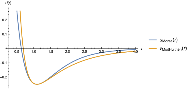
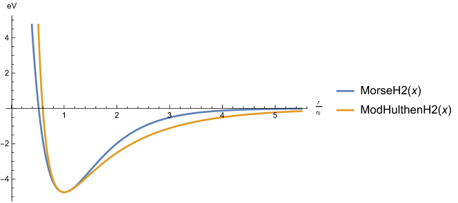
A graphical example, comparing both potentials, when $V_{0}=a=1\/,$ $b=2\/,$ and $r_{\text{min}}=\ln 3\simeq 1.09861\/,$ is presented in Figure 2 and further discussed in our Mathematica notebook for the reader’s convenience, as well as potentials for molecules $\text{H}_{2}\/$ , HCl, and $\text{I}_{2}\/$ with a completion of the data from [10] in Table 15 (see also Figure 3).

Table 15. Comparison of the parameters for the Morse potential and the modified Hulthén potential:

E(

)=E(

{}^{-1})\times 1.2398\times 10^{-4}

according to [10].

Molecule	${\dfrac{\hbar^{2}}{2mr_{0}^{2}}}\ ($ cm ${}^{-1})$	$D\ ($ cm ${}^{-1})$	$\alpha$	$b$	$V_{0}\ ($ cm ${}^{-1})$
H₂	$60.8296$	$38292$	$1.440$	$1.5904$	$67394$
HCl	$10.5930$	$37244$	$2.380$	$4.51744$	$5\allowbreak 24010$
I₂	$0.0374$	$12550$	$4.954$	$68.848$	$1984\,90$

In order to find parameters of the modified Hulthén potential in terms of the Morse ones, we have solved numerically the following equation:

(17.44)

\alpha=\varphi(b):=\frac{(2b-1)\ln(2b-1)}{2(b-1)},\quad b\geq 1

with the monotone function $\varphi(b).$ Then $V_{0}=4(b-1)D$ and $a=r_{0}/\ln(2b-1).$ (More details are provided in the Mathematica file.)

Remark. The so-called generalized Morse potential is usually introduced as

(17.45)

U(r)=D\left(1-\frac{e^{\alpha r_{0}}-1}{e^{\alpha r}-1}\right)^{2}

( $D,$ $\alpha,$ $r_{0}$ are parameters) with the following asymptotic

(17.46)

U(\infty)=\lim_{r\rightarrow\infty}U(r)=D>0

(see [9], [31], and the references therein). The difference

(17.47)

U(r)-U(\infty)=-2D\left(e^{\alpha r_{0}}-1\right)\ \frac{1-e^{-\alpha r}\left(1+e^{\alpha r_{0}}\right)/2}{\left(1-e^{-\alpha r}\right)^{2}}e^{-\alpha r}

has the form of our modified Hulthén potential (17.1) with the parameters given by

(17.48)

V_{0}=2D\left(e^{\alpha r_{0}}-1\right),\quad b=\frac{1}{2}\left(1+e^{\alpha r_{0}}\right),\quad a=\frac{1}{\alpha}.

Therefore, this case has been studied here as well (see also section 19 for an independent computer algebra approach).

Table 16. The modified Hulthén potential (17.1) in the spherically symmetric case

l=0

. Substitution:

R(r)=u(\xi)

\xi=\exp(-r/a)

\alpha^{2}=-(2mE/\hbar^{2})\ a^{2}>0

\beta^{2}=(2mV_{0}/\hbar^{2})\ a^{2}>0

$\sigma(\xi)$	$\xi(1-\xi)$
$\widetilde{\sigma}(\xi)$	$-\left({\alpha}^{2}+b{\beta}^{2}\right){\xi}^{2}+\left(2{\alpha}^{2}+{\beta}^{2}\right)\xi-{\alpha}^{2}$
$\widetilde{\tau}(\xi)$	$1-\xi$
$k$	${\beta^{2}}-2\alpha\kappa,\qquad\kappa=\sqrt{(1/4)+(b-1){\beta}^{2}}$
$\pi(\xi)$	$\alpha-(\alpha+\kappa+1/2)\xi$
$\tau(\xi)=\widetilde{\tau}+2\pi$	$2\alpha+1-2(\alpha+\kappa+1)\xi$
$\lambda=k+\pi^{\prime}$	${\beta}^{2}-(2\alpha+1)(\kappa+1/2)$
$\varphi(\xi)$	$\xi^{\alpha}(1-\xi)^{\kappa+1/2}$
$\rho(\xi)$	$\xi^{2\alpha}(1-\xi)^{2\kappa}$
$E_{n}$	$-V_{0}\left(\dfrac{b\beta^{2}-(n+\kappa+1/2)^{2}}{2\beta(n+\kappa+1/2)}\right)^{2}\/,\;n=0,1,2,\ \dots\;\left(n\leq n_{\rm{max}}\right)$
$y_{n}(\xi)$	${}_{2}F_{1}(-n,\,2\alpha+2\kappa+n+1;\,2\alpha+1;\,\xi)$ ,
	$\alpha={\dfrac{b\beta^{2}-(n+\kappa+1/2)^{2}}{2(n+\kappa+1/2)}>0}$
$C_{n}^{2}$	$\dfrac{\Gamma(2\alpha+n+1)\Gamma(2\alpha+2\kappa+n+1)(2\alpha+2\kappa+2n+1)}{a(2\alpha)\Gamma^{2}(2\alpha)\Gamma(2\kappa+n+1)(2\kappa+2n+1)n!}$

18. Rotation Correction of Modified Hulthén Potential

In view of

(18.1)

\frac{dU(r)}{dr}=V_{0}\ e^{r/a}\frac{1-2b+e^{r/a}}{a\left(e^{r/a}-1\right)^{3}}=0,

the minimum of the modified Hulthén potential (17.1) occurs when

(18.2)

e^{r_{\text{min}}/a}=2b-1>1.

By letting $r=a(1+x)x_{0}\/$ in the neighborhood of this minimum $r\approx r_{\text{min}}$ (or $x\approx 0$ ), with the aid of Mathematica, we derive the following expansion:

(18.3)		$\displaystyle\frac{1}{(1+x)^{2}}-C_{0}-e^{-(1+x)x_{0}}\frac{C_{1}+C_{2}e^{-(1+x)x_{0}}}{\left(1-e^{-(1+x)x_{0}}\right)^{2}}$
	$\displaystyle\quad=\left(-4+\frac{3bx_{0}}{b-1}-\frac{1-2b+4b^{2}}{6(b-1)^{2}}x_{0}^{2}\right)x^{3}+\text{O}(x^{4}),\quad x\rightarrow 0,$

where

(18.4)		$\displaystyle C_{0}$	$\displaystyle=1+4(b-1)\frac{3(b-1)-(3b-1)x_{0}}{(2b-1)^{2}x_{0}^{2}},$
	$\displaystyle C_{1}$	$\displaystyle=8(b-1)^{2}\frac{6(1-b)+(4b-1)x_{0}}{(2b-1)^{2}x_{0}^{2}},$
	$\displaystyle C_{2}$	$\displaystyle=8(b-1)^{2}\frac{6b(b-1)+(1-2b(b+1))x_{0}}{(2b-1)^{2}x_{0}^{2}}$

and $e^{x_{0}}=2b-1>1$ (see our complementary Mathematica file).

Therefore,

(18.5)

\frac{l(l+1)}{r^{2}}\approx{\frac{l(l+1)}{r^{2}_{\text{min}}}}\left[C_{0}+e^{-r/a}\frac{C_{1}+C_{2}e^{-r/a}}{\left(1-e^{-r/a}\right)^{2}}\right]\qquad(r_{\text{min}}=ax_{0})\/,{}

and our equation (17.2) for the modified Hulthén potential holds, once again, but with the following modified values of the parameters:

	$\displaystyle\alpha^{2}$	$\displaystyle\rightarrow\alpha_{1}^{2}=\alpha^{2}+\frac{l(l+1)}{x_{0}^{2}}C_{0},$	$\displaystyle\quad\beta^{2}$	$\displaystyle\rightarrow\beta_{1}^{2}=\beta^{2}-\frac{l(l+1)}{x_{0}^{2}}C_{1},$
(18.6)		$\displaystyle b$	$\displaystyle\rightarrow b_{1}=\frac{\beta_{2}^{2}}{\beta_{1}^{2}},$	$\displaystyle\quad\beta_{2}^{2}$	$\displaystyle=b\beta^{2}+{\frac{l(l+1)}{x_{0}^{2}}}C_{2},$

namely,

(18.7)

\xi^{2}\frac{d^{2}u}{d\xi^{2}}+\xi\frac{du}{d\xi}+\left[-{\alpha_{1}^{2}}+{\beta_{1}^{2}}\ \frac{\xi\left(1-b_{1}\xi\right)}{\left(1-\xi\right)^{2}}\right]u=0.\/{}

As a result, we have arrived at the generalized equation of hypergeometric type (Table 17) and our analysis from the previous section is valid, say, up to a proper change of parameters.

For example, the vibration and rotation energy levels are given by

(18.8)		$\displaystyle E_{v,l}$	$\displaystyle=-V_{0}\left(\frac{\beta_{2}^{2}-\left(\kappa_{1}+v+1/2\right)^{2}}{2\beta\left(\kappa_{1}+v+1/2\right)}\right)^{2}$
		$\displaystyle\quad\;+\frac{\hbar^{2}l(l+1)}{2mr_{\text{min}}^{2}}\left[1+4(b-1)\frac{3(b-1)-(3b-1)x_{0}}{(2b-1)^{2}x_{0}^{2}}\right]{}$

( $v=0,1,2,\ \dots\ \leq v_{\text{max}}\/$ ). Here,

(18.9)

{\beta_{2}^{2}-\left(\kappa_{1}+v+\dfrac{1}{2}\right)^{2}}=\beta_{1}^{2}-v^{2}-(2\kappa_{1}+1)\left(v+\dfrac{1}{2}\right)>0\/.{}

The corresponding normalized wave functions are the same as before in (17.18) and (17.40) but with the new values of parameters (18.6) (we leave further details to the reader).

Our study of the rotation correction of the modified Hulthén potential will be continued elsewhere (see also the Mathematica file).

Table 17. The rotation correction of the modified Hulthén potential (18.5), where the coefficients

C_{0}

C_{1}

, and

C_{2}

are given by (18.4).

$\sigma(\xi)$	$\xi(1-\xi)$
$\widetilde{\sigma}(\xi)$	$-\left({\alpha}^{2}_{1}+b_{1}{\beta}^{2}_{1}\right){\xi}^{2}+\left(2{\alpha}^{2}_{1}+{\beta}^{2}_{1}\right)\xi-{\alpha}^{2}_{1}$
$\widetilde{\tau}(\xi)$	$1-\xi$
$k$	${\beta}_{1}^{2}-2{\alpha}_{1}{\kappa}_{1}\/,\quad{\kappa}_{1}=\sqrt{(1/4)+(b_{1}-1){\beta}_{1}^{2}}$
$\pi(\xi)$	${\alpha}_{1}-({\alpha}_{1}+{\kappa}_{1}+1/2)\xi$
$\tau(\xi)=\widetilde{\tau}+2\pi$	$(2{\alpha}_{1}+1)-2({\alpha}_{1}+{\kappa}_{1}+1)\xi$
$\lambda=k+\pi^{\prime}$	${\beta}_{1}^{2}-\left(2{\alpha}_{1}+1\right)\left({\kappa}_{1}+1/2\right)$
$\varphi(\xi)$	$\xi^{\alpha_{1}}(1-\xi)^{\kappa_{1}+1/2}$
$\rho(\xi)$	$\xi^{2\alpha_{1}}(1-\xi)^{2\kappa_{1}}$

19. Generalized Morse Potential

The potential of the form:

(19.1)

U(r)=D\left(1-\frac{\gamma}{e^{ar}-1}\right)^{2},\quad\gamma=e^{ar_{0}}-1\quad\quad\left(0\leq r<\infty\right){}

by (17.47) is reduced to the modified Hulthén potential (17.1) up to a proper change of parameters (17.48). This is why, we can use solutions from section 17.

On the second thought, the standard change of the variables [9]:

(19.2)

R(r)=\sqrt{a}u(\eta),\qquad\eta=\left(e^{ar}-1\right)^{-1}{}

results in the generalized equation of hypergeometric type with the following coefficients:

(19.3)

\sigma(\eta)=\eta(1+\eta),\quad\widetilde{\sigma}(\eta)=\epsilon-\kappa(1-\gamma\eta)^{2},\quad\widetilde{\tau}(\eta)=2\eta+1,

where

(19.4)

\kappa=\frac{2mD}{a^{2}\hbar^{2}},\quad\epsilon=\frac{2mE}{a^{2}\hbar^{2}};\qquad{\alpha}^{2}=\kappa-\epsilon>0,\quad{\beta}^{2}=\kappa(\gamma+1)^{2}-\epsilon>0

(see Table 18 and the Mathematica file). The following substitution

(19.5)

u=\varphi(\eta)y(\eta)=\frac{\eta^{\alpha}}{(1+\eta)^{\beta}}y(\eta)

results in the hypergeometric equation of Gauss (14.13) in the variable $-\eta$ with the following values of parameters:

(19.6)

A=\alpha-\beta+\delta,\quad B=\alpha-\beta-\delta+1,\quad C=2\alpha+1;\quad\delta=\frac{1}{2}+\sqrt{\frac{1}{4}+\kappa\gamma^{2}}.

Bound states correspond to the polynomial solutions, when $A=\alpha-\beta+\delta=-n$ and $n$ are some nonnegative integers. Thus $\alpha$ and $\beta$ are $n$ -dependent, once again, and satisfy the following equations:

(19.7)

\beta_{n}-\alpha_{n}=n+\delta,\qquad\beta_{n}^{2}-\alpha_{n}^{2}=\kappa\gamma(\gamma+2).

One finds that

(19.8)

\alpha_{n}=\frac{1}{2}\left(\frac{\kappa\gamma(\gamma+2)}{n+\delta}-n-\delta\right),\quad\beta_{n}=\frac{1}{2}\left(\frac{\kappa\gamma(\gamma+2)}{n+\delta}+n+\delta\right)

and the energy levels have the form [9]:

(19.9)

E_{n}=D-\frac{\alpha^{2}\hbar^{2}}{8m}\left(n+\delta-\frac{\kappa\gamma(\gamma+2)}{n+\delta}\right)^{2}.

The corresponding normalized wave functions are given by

(19.12)		$\displaystyle R_{n}(r)$	$\displaystyle=\sqrt{a}C_{n}e^{-{\beta_{n}}ar}\left(e^{ar}-1\right)^{{\beta_{n}}-{\alpha_{n}}}\ _{2}F_{1}\left(\begin{array}[]{c}-n,\ 1-n-2\delta\\ 2\alpha_{n}+1\end{array};\frac{1}{1-e^{ar}}\right)$
(19.15)			$\displaystyle=\sqrt{a}C_{n}e^{-{\alpha_{n}}ar}\left(1-e^{-ar}\right)^{\delta}\ _{2}F_{1}\left(\begin{array}[]{c}-n,\ 2{\alpha_{n}}+2\delta+n\\ 2{\alpha_{n}}+1\end{array};e^{-ar}\right)$

[we have used (15.8.1) of [28]) in order to obtain the standard form (17.18)], with the normalization coefficients found in [9] as follows

(19.16)

C_{n}^{2}=\frac{a(\alpha_{n}+n+\delta)\Gamma(2\alpha_{n}+n+1)\Gamma(2\alpha_{n}+n+2\delta)}{n!(n+\delta)\Gamma(2\alpha_{n})\Gamma(2\alpha_{n}+1)\Gamma(n+2\delta)}\/,

due to the normalization condition:

(19.17)

\int_{0}^{\infty}R_{n}^{2}(r)\ dr=1\/.

There is only a finite set of the energy levels:

(19.18)

n=0,1,2,\ \ldots\ n_{\text{max}}\leq\sqrt{\kappa\gamma(\gamma+2)}-\delta.

One can use our results from section 17 in order to verify all these formulas, originally presented in [9] (see also [1], [31], and the references therein). We leave further details to the reader.

Table 18. The generalized Morse potential (19.1). The coefficients

\epsilon\/

and

\kappa

are given by (19.4).

$\sigma(\eta)$	$\eta(1+\eta)$
$\widetilde{\sigma}(\eta)$	$\epsilon-\kappa\left(1-\gamma\eta\right)^{2}$
$\widetilde{\tau}(\eta)$	$2\eta+1$
$k$	$2\left(\alpha^{2}-\alpha\beta+\kappa\gamma\right)\/,\quad{{\alpha=\sqrt{\kappa-\epsilon}}\ },\;\beta=\sqrt{\kappa(\gamma+1)^{2}-\epsilon}$
$\pi(\eta)$	${\alpha}+({\alpha}-{\beta})\eta$
$\tau(\eta)=\widetilde{\tau}+2\pi$	$2{\alpha}+1+2({\alpha}-{\beta}+1)\eta$
$\lambda=k+\pi^{\prime}$	$\alpha-\beta+2{\alpha}^{2}-2\alpha\beta+2\kappa\gamma$
$\varphi(\eta)$	$\eta^{\alpha}(1+\eta)^{-\beta}$
$\rho(\eta)$	$\eta^{2\alpha}(1+\eta)^{-2\beta}$

In a similar fashion, one can consider the Wood–Saxon potential and the motion of the electron in magnetic field [1], [9], [10], [15] [23], and [27].

Acknowledgments. We are grateful to Dr. Steven Baer, Dr. Kamal Barley, Dr. Sergey Kryuchkov, Dr. Eugene Stepanov, Dr. José Vega-Guzmán, and Dr. Alexei Zhedanov for valuable discussions and help.

Appendix A Data for the Classical Orthogonal Polynomials

The basic information about classical orthogonal polynomials, namely, for the Jacobi ${P_{n}^{(\alpha,\beta)}(x)}\/,$ Laguerre ${L_{n}^{\alpha}(x)}\/,$ and Hermite $H_{n}(x)$ polynomials, is presented, for the reader’s convenience, in Table 19. It contains the coefficients of the differential equation (2.3), the intervals of orthogonality $(a,b)$ , the weight functions $\rho(x)$ and constants $B_{n}$ in the Rodrigues-type formula (2.8), the leading terms:

(A.1)

y_{n}(x)=a_{n}x^{n}+b_{n}x^{n-1}+\ldots

for these polynomials, their squared norms:

(A.2)

d_{n}^{2}=\int_{a}^{b}y_{n}^{2}(x)\rho(x)\,dx,

and the coefficients of the three-term recurrence relation:

(A.3)

x\,y_{n}(x)=\alpha_{n}\,y_{n+1}(x)+\beta_{n}\,y_{n}(x)+\gamma_{n}\,y_{n-1}(x),

where

(A.4)

\alpha_{n}=\frac{a_{n}}{a_{n+1}},\quad\beta_{n}=\frac{b_{n}}{a_{n}}-\frac{b_{n+1}}{a_{n+1}},\quad\gamma_{n}=\alpha_{n-1}\,\frac{d_{n}^{2}}{d_{n-1}^{2}}.

(More details can be found in [2], [26], [27], [28], and [42].)

Table 19. Data for the Jacobi

{P_{n}^{(\alpha,\beta)}(x)}\/,

Laguerre

{L_{n}^{\alpha}(x)}\/,

and Hermite

H_{n}(x)

polynomials.

$y_{n}(x)$	$P_{n}^{(\alpha,\,\beta)}(x)\,(\alpha>-1,\beta>-1)$	$L_{n}^{\alpha}(x)\,(\alpha>-1)$	$H_{n}(x)$
$(a,b)$	$(-1,1)$	$(0,\infty)$	$(-\infty,\infty)$
$\rho(x)$	$(1-x)^{\alpha}(1+x)^{\beta}$	$x^{\alpha}\,e^{-x}$	$e^{-x^{2}}$
$\sigma(x)$	$1-x^{2}$	$x$	$1$
$\tau(x)$	$\beta-\alpha-(\alpha+\beta+2)\,x$	$1+\alpha-x$	$-2x$
$\lambda_{n}$	$n(\alpha+\beta+n+1)$	$n$	$2n$
$B_{n}$	$\dfrac{(-1)^{n}}{2^{n}n!}$	$\dfrac{1}{n!}$	$(-1)^{n}$
$a_{n}$	$\dfrac{\Gamma(\alpha+\beta+2n+1)}{2^{n}n!\Gamma(\alpha+\beta+n+1)}$	$\dfrac{(-1)^{n}}{n!}$	$2^{n}$
$b_{n}$	$\dfrac{(\alpha-\beta)\Gamma(\alpha+\beta+2n)}{2^{n}(n-1)!\Gamma(\alpha+\beta+n+1)}$	$(-1)^{n-1}\dfrac{\alpha+n}{(n-1)!}$	$0$
$d^{2}$	$\dfrac{2^{\alpha+\beta+1}\Gamma(\alpha+n+1)\Gamma(\beta+n+1)}{n!(\alpha+\beta+2n+1)\Gamma(\alpha+\beta+n+1)}$	$\dfrac{\Gamma(\alpha+n+1)}{n!}$	$2^{n}n!\sqrt{\pi}$
$\alpha_{n}$	$\dfrac{2(n+1)(\alpha+\beta+n+1)}{(\alpha+\beta+2n+1)(\alpha+\beta+2n+2)}$	$-(n+1)$	$\dfrac{1}{2}$
$\beta_{n}$	$\dfrac{\beta^{2}-\alpha^{2}}{(\alpha+\beta+2n)(\alpha+\beta+2n+2)}$	$\alpha+2n+1$	$0$
$\gamma_{n}$	$\dfrac{2(\alpha+n)(\beta+n)}{(\alpha+\beta+2n)(\alpha+\beta+2n+1)}$	$-(\alpha+n)$	$n$

Appendix B An Integral Evaluation

The following useful integral:

(B.1)	$\displaystyle J_{nms}^{\alpha\beta}$	$\displaystyle=\int_{0}^{\infty}e^{-x}x^{\alpha+s}\ L_{n}^{\alpha}(x)L_{m}^{\beta}(x)\ dx$
	$\displaystyle=(-1)^{n-m}\frac{\Gamma(\alpha+s+1)\,\Gamma(\beta+m+1)\,\Gamma(s+1)}{m!\,(n-m)!\,\Gamma(\beta+1)\,\Gamma(s-n+m+1)}$
(B.4)		$\displaystyle\quad\times\ _{3}F_{2}\biggl{(}\begin{array}[]{@{}c@{}}-m,\ s+1,\ \beta-\alpha-s\\ \beta+1,\quad n-m+1\end{array};1\biggr{)},\quad n\geq m,$

where parameter $s$ may take some integer values and ${}_{3}F_{2}(1)$ is the generalized hypergeometric series [2], [28], has been evaluated in [41] and [42] (see also [13], [35]). Special cases have been used above for the normalization of the wave functions; see (7.13) and (15.22).

We use also throughout the manuscript the familiar Euler beta and gamma integrals:

(B.5)

B(\alpha,\ \beta)=\int_{0}^{1}t^{\alpha-1}(1-t)^{\beta-1}\ dt=\dfrac{\Gamma(\alpha)\Gamma(\beta)}{\Gamma(\alpha+\beta)}\/,

provided $\Re{(\alpha)}>0$ and $\Re{(\alpha)}>0\/,$

(B.6)

\Gamma(\alpha)=\int_{0}^{\infty}t^{\alpha-1}e^{-t}\ dt\/,\qquad\Re{(\alpha)}>0.

(See [2], [27], and [28] for more details.)

Appendix C Mathematica File

We have discussed basic potentials of the nonrelativistic and relativistic quantum mechanics that can be integrated in the Nikiforov and Uvarov paradigm with the aid of the Mathematica computer algebra system. (The corresponding Mathematica notebook is available from the authors by a request. It is also posted on Wolfram community https://community.wolfram.com/groups/-/m/t/2897057 and featured in the editorial columns https://community.wolfram.com/content?curTag=staff+picks .)

In section 2, the general formulas are derived. In the notebook, they are stored in global variables that will be used in all the subsequent sections. For this purpose, allow Mathematica to evaluate all initialization cells. After that one can run each case independently from the others. The results, for the most integrable cases that are available in the literature, are presented in the Tables 1–18.

References

[1] A. B. Al-Othman and A. S. Sandouqa, Comparison study of bound states for diatomic molecules using Kratzer, Morse, and modified Morse potentials, Physica Scripta, 97(3), 035401, 2022. https://doi.org/10.1088/1402-4896/ac514c.
[2] G. E. Andrews, R. Askey, and R. Roy, Special Functions, Cambridge University Press, New York, 1999.
[3] K. Barley, J. Vega-Guzmán, A. Ruffing, and S. K. Suslov, Discovery of the relativistic Schrödinger equation, Physics–Uspekhi, 69(1), 90–103, 2022 [in English]; 192(1), 100–114, 2022 [in Russian]; https://iopscience.iop.org/article/10.3367/UFNe.2021.06.039000.
[4] H. A. Bethe and E. Salpeter, Quantum Mechanics of One- and Two-Electron Atoms, Dover Publications, Mineola, New York, 2008.
[5] C. Berkdemir, A. Berkdemir, and J. Han, Bound state solutions of the Schrödinger equation for modified Kratzer’s potential, Chemical Physics Letters 417(4–6), 326–329, 2006. https://www.sciencedirect.com/science/article/abs/pii/S0009261405015812.
[6] D. I. Blokhintsev, Quantum Mechanics, D. Reidel, Dordrecht, 1964.
[7] A. S. Davydov, Quantum Mechanics, Pergamon Press, Oxford and New York, 1965.
[8] C. G. Darwin, The wave equations of the electron, Proceedings of the Royal Society A: Mathematical, Physical and Engineering Sciences 118(780), 654–680, 1928. https://doi.org/10.1098/rspa.1928.0076
[9] A. Del Sol Mesa, C. Quesne, and Yu. F. Smirnov, Generalized Morse potential: Symmetry and satellite potentials, Journal of Physics A: Mathematical and General 31(1), 321–335, 1998. https://iopscience.iop.org/article/10.1088/0305-4470/31/1/028
[10] S. Flügge, Practical Quantum Mechanics, Springer-Verlag, Berlin, Hedelberg, New York, 1999.
[11] S. Flügge, P. Walger, and A. Weiguny, A generalization of the Morse potential, Journal of Molecular Spectroscopy 23(3), 243–257, 1967. https://doi.org/10.1016/S0022-2852(67)80013-4
[12] V. A. Fock, Fundamentals of Quantum Mechanics, Moscow: Mir Publishers, 1978. https://mirtitles.org/2013/01/01/fock-fundamentals-of-quantum-mechanics/.
[13] E. Fues, Das Eigenschwingungsspektrum zweiatomiger Moleküle in der Undulationsmechanik, Annalen der Physik 385(12), 367–396, 1926. https://onlinelibrary.wiley.com/doi/10.1002/andp.19263851204 [in German].
[14] I. I. Gol’dman and V. D. Krivchenkov, Problems in Quantum Mechanics, Dover Publications, Inc., New York, 1993.
[15] B. Gönül and K. Köksal, Solutions for a generalized Woods-Saxon potential, Physica Scripta 76(5), 565–570 (2007). http://dx.doi.org/10.1088/0031-8949/76/5/026
[16] W. Gordon, Die Energieniveaus des Wasserstoffatoms nach der Diracschen Quantentheorie des Elektrons, Zeitschrift für Physik 48(1), 11–14, 1928. https://doi.org/10.1007/BF01351570 [in German]
[17] W. Greiner, Relativistic Quantum Mechanics: Wave Equations, 2nd ed., Springer-Verlag, Berlin and Hedelberg, 1997.
[18] M. Karplus and R. N. Porter, Atoms & Molecules: An Introduction for Students of Physical Chemistry, The Benjamin/Cummings Company, Menlo Park, California, 1970.
[19] C. Koutschan, E. Suazo, and S. K. Suslov, Fundamental laser modes in paraxial optics: from computer algebra and simulations to experimental observation. Applied Physics B 121(3), 315–336, 2015. https://doi.org/10.1007/s00340-015-6231-9
[20] C. Koutschan and D. Zeilberger, The 1958 Pekeris–Accad–WEIZAC ground-breaking collaboration that computed ground states of two-electron atoms (and its 2010 redux), Mathematical Intelligencer 33, 52–57, 2011. https://doi.org/10.1007/s00283-010-9192-1
[21] S. I. Kryuchkov, S. K. Suslov, and J. M. Vega-Guzmán, The minimum-uncertainty squeezed states for atoms and photons in a cavity. Journal of Physics B: Atomic, Molecular and Optical Physics 46(10), 104007 (2013). https://iopscience.iop.org/article/10.1088/0953-4075/46/10/104007
[22] R. E. Langer, On the connection formulas and the solutions of the wave equation, Physical Review 51 no. 8 (1937), 669–676. https://journals.aps.org/pr/abstract/10.1103/PhysRev.51.669
[23] L. D. Landau and E. M. Lifshitz, Quantum Mechanics: Non-Relativistic Theory, 3rd ed., Butterworth–Heinemann, Oxford, 1998.
[24] R. M. López, S. K. Suslov, and J. M. Vega-Guzmán, On a hidden symmetry of quantum harmonic oscillators. Journal of Difference Equations and Applications 19(4), 543–554, 2013. https://www.tandfonline.com/doi/abs/10.1080/10236198.2012.658384
[25] P. M. Morse, Diatomic molecules according to the wave mechanics. II. Physical Review 34(1), 57–64, 1929. https://journals.aps.org/pr/abstract/10.1103/PhysRev.34.57
[26] A. F. Nikiforov, S. K. Suslov, and V. B. Uvarov, Classical Orthogonal Polynomials of a Discrete Variable, Springer Series in Computational Physics. Springer Berlin Heidelberg, Berlin, Heidelberg, 1991.
[27] A. F. Nikiforov and V. B. Uvarov, Special Functions of Mathematical Physics: A Unified Introduction with Applications, Birkhäuser, Boston, MA, 1988.
[28] NIST Handbook of Mathematical Functions, (F. W. J. Olver and D. W. Lozier, eds.), Cambridge University Press, New York, 2010. https://dlmf.nist.gov/.
[29] C. L. Pekeris. Ground state of two-electron atoms, Physical Review 112(5), 1649–1658, 1958. https://doi.org/10.1103/PhysRev.112.1649.
[30] G. Pöschl and E. Teller, Bemerkungen zur Quantenmechanik des anharmonischen Oszillators. Zeitschrift für Physik 83 March issue, 143–151 (1933), https://doi.org/10.1007/BF01331132.
[31] Z. Rong, H. G. Kjaergaard, and M. L. Sage, Comparison of the Morse and Deng–Fan potentials for X–H bonds in small molecules, Molecular Physics 101(14), 2285–2294, 2003. https://www.tandfonline.com/doi/abs/10.1080/0026897031000137706
[32] N. Rosen and P. M. Morse, On the Vibrations of Polyatomic Molecules. Phys. Rev. 42 (2), 210–217 (1932), https://doi.org/10.1103/PhysRev.42.210.
[33] E. Schrödinger, Quantisation as a problem of proper values (Part I), in Collected Papers on Wave Mechanics, New York, Providence, Rhode Island: AMS Chelsea Publishing, 2010, (Original: Annalen der Physik (4), vol. 79(6), pp. 489–527, 1926 [in German]), pp. 1–12. https://onlinelibrary.wiley.com/doi/10.1002/andp.19263840404
[34] E. Schrödinger, Quantisation as a problem of proper values (Part II), in Collected Papers on Wave Mechanics, New York, Providence, Rhode Island: AMS Chelsea Publishing, 2010, (Original: Annalen der Physik (4), vol. 79(6), pp. 489–527, 1926 [in German]), pp. 13–40. https://onlinelibrary.wiley.com/doi/10.1002/andp.19263840602
[35] E. Schrödinger, Quantisation as a problem of proper values (Part III), in Collected Papers on Wave Mechanics, New York, Providence, Rhode Island: AMS Chelsea Publishing, 2010, (Original: Annalen der Physik (4), vol. 386 # 18, pp. 109–139, 1926 [in German]), pp. 62–101. https://onlinelibrary.wiley.com/doi/abs/10.1002/andp.19263851302.
[36] E. Schrödinger, The continuous transition from micro-to macro-mechanics, in Collected Papers on Wave Mechanics, 28, New York, Providence, Rhode Island: AMS Chelsea Publishing, 2010, (Original: Die Naturwissenschaften, vol. 28, pp. 664–666, 1926 [in German]), pp. 41–44. https://doi.org/10.1007/BF01507634
[37] E. Schrödinger, Quantisation as a problem of proper values (Part IV), in Collected Papers on Wave Mechanics, New York, Providence, Rhode Island: AMS Chelsea Publishing, 2010, (Original: Annalen der Physik (4), vol. 81, pp. 109–139, 1926 [in German]), pp. 102–123. https://onlinelibrary.wiley.com/doi/10.1002/andp.19263861802.
[38] E. Schrödinger, An undulatory theory of the mechanics of atoms and molecules, Physical Review 28(6), 1049–1070, 1926. https://journals.aps.org/pr/abstract/10.1103/PhysRev.28.1049.
[39] L. I. Schiff, Quantum Mechanics, 3rd edn. International series in pure and applied physics. McGraw-Hill, Inc., New York, 1968.
[40] A. Sommerfeld, Atombau und Spektrallinien, 2 ed., 1, Friedrich Vieweg & Sohn, Braunschweig, German, 1951. [in German]
[41] S. K. Suslov and B. Trey, The Hahn polynomials in the nonrelativistic and relativistic Coulomb problems. Journal of Mathematical Physics 49(1), 012104 (2008). https://doi.org/10.1063/1.2830804
[42] S. K. Suslov, J. M. Vega-Guzmán, and K. Barley, An introduction to special functions with some applications to quantum mechanics, in Orthogonal Polynomials: 2nd AIMS-Volkswagen Stiftung Workshop, Douala, Cameroon, 5-12 October, 2018 (M. Foupouagnigni and W. Koepf, eds.), Tutorials, Schools, and Workshops in the Mathematical Sciences no. AIMSVSW 2018, Springer Nature Switzerland AG, March 2020, pp. 517–628. https://link.springer.com/chapter/10.1007/978-3-030-36744-2_21
[43] D. A. Varshalovich, A. N. Moskalev, and V. K. Khersonskii, Quantum Theory of Angular Momentum, Singapore, New Jersey, Hong Kong: World Scientific, 1988.
[44] G. N. Watson, A Treatise on the Theory of Bessel Functions, 2nd edn. Cambridge Mathematical Library. Cambridge University Press, Cambridge, England, 1995. [Reprint of the second (1944) edition]
[45] E. T. Whittaker and G. N. Watson, A Course of Modern Analysis: An Introduction to the General Theory of Infinite Processes and of Analytic Functions; with an Account of the Principal Transcendental Functions. Cambridge Mathematical Library. Cambridge University Press, Cambridge, England, 1950. [Reprint of the 4th (1927) edition]