This paper was converted on www.awesomepapers.org from LaTeX by an anonymous user.
Want to know more? Visit the Converter page.

On Regularization of Gradient Descent,
Layer Imbalance and Flat Minima

Boris Ginsburg
NVIDIA, Santa Clara, CA USA
bginsburg@nvidia.com
Abstract

We analyze the training dynamics for deep linear networks using a new metric – layer imbalance – which defines the flatness of a solution. We demonstrate that different regularization methods, such as weight decay or noise data augmentation, behave in a similar way. Training has two distinct phases: 1) ‘optimization’ and 2) ‘regularization’. First, during the optimization phase, the loss function monotonically decreases, and the trajectory goes toward a minima manifold. Then, during the regularization phase, the layer imbalance decreases, and the trajectory goes along the minima manifold toward a flat area. Finally, we extend the analysis for stochastic gradient descent and show that SGD works similarly to noise regularization.

1 Introduction

In this paper, we analyze regularization methods used for training of deep neural networks. To understand how regularization like weight decay and noise data augmentation work, we study gradient descent (GD) dynamics for deep linear networks (DLNs). We study deep networks with scalar layers to exclude factors related to over-parameterization and to focus on factors specific to deep models. Our analysis is based on the concept of flat minima [5]. We call a region in weight space flat, if each solution from that region has a similar small loss. We show that minima flatness is related to a new metric, layer imbalance, which measures the difference between the norm of network layers. Next, we analyze layer imbalance dynamics of gradient descent (GD) for DLNs using a trajectory-based approach [10].

With these tools, we prove the following results:

  1. 1.

    Standard regularization methods such as weight decay and noise data augmentation, decrease layer imbalance during training and drive trajectory toward flat minima.

  2. 2.

    Training for GD with regularization has two distinct phases: (1) ‘optimization’ and (2) ‘regularization’. During the optimization phase, the loss monotonically decreases, and the trajectory goes toward minima manifold. During the regularization phase, layer imbalance decreases and the trajectory goes along minima manifold toward flat area.

  3. 3.

    Stochastic Gradient Descent (SGD) works similarly to implicit noise regularization.

2 Linear neural networks

We begin with a linear regression y=wx+by=w\cdot x+b with mean squared error on scalar samples {xi,yi}\{x_{i},y_{i}\}:

E(w,b)=1N(wxi+byi)2minE(w,b)=\frac{1}{N}\sum(w\cdot x_{i}+b-y_{i})^{2}\rightarrow min (1)

Let’s center and normalize the training dataset in the following way:

xi=0;1Nxi2=1;\displaystyle\sum x_{i}=0;\;\;\frac{1}{N}\sum x^{2}_{i}=1; yi=0;1Nxiyi=1.\displaystyle\sum y_{i}=0;\;\;\frac{1}{N}\sum x_{i}y_{i}=1. (2)

The solution for this normalized linear regression is (w,b)=(1,0)(w,b)=(1,0).

Next, let’s replace y=wx+by=w\cdot x+b with a linear network with dd scalar layers 𝒘=(w1,,wd){\bm{w}}=(w_{1},\dots,w_{d}):

y=w1wdx+b\displaystyle y=w_{1}\cdots w_{d}\cdot x+b (3)

Denote 𝐖:=𝐰𝟏𝐰𝐝\mathbf{W:=w_{1}\cdots w_{d}}. The loss function for the new problem is:

E(𝒘,b)=1N(Wxi+byi)2minE({\bm{w}},b)=\frac{1}{N}\sum(W\cdot x_{i}+b-y_{i})^{2}\rightarrow min

Now the loss E(𝒘,.)E({\bm{w}},.) is a non-linear (and non-convex) function with respect to the weights 𝒘{\bm{w}}. For the normalized dataset (2), network training is equivalent to the following problem:

L(𝒘)=(w1wd1)2minL({\bm{w}})=(w_{1}\cdots w_{d}-1)^{2}\rightarrow\min (4)

Such linear networks with depth-2 have been studied in Baldi and Hornik [2], who showed that all minima for the problem (4) are global and that all other critical points are saddles.

2.1 Flat minima

Following Hochreiter et al [5], we are interested in flat minima – “a region in weight space with the property that each weight from that region has similar small error". In contrast, sharp minima are regions where the function can increase rapidly. Let’s compute the loss gradient L(𝒘)\nabla L({\bm{w}}):

Lwi\displaystyle\frac{\partial L}{\partial w_{i}} =2(w1wd1)(w1wi1wi+1wd)=2(W1)(W/wi)\displaystyle=2(w_{1}\cdots w_{d}-1)(w_{1}\cdots w_{i-1}w_{i+1}\cdots w_{d})=2(W-1)(W/w_{i}) (5)

Here we denote 𝐖/𝐰𝐢:=𝐰𝟏𝐰𝐢𝟏𝐰𝐢+𝟏𝐰𝐝\mathbf{W/w_{i}:=w_{1}\cdots w_{i-1}\cdot w_{i+1}\cdots w_{d}} for brevity. The minima of loss LL are located on hyperbola w1wd=1w_{1}\cdots w_{d}=1 (Fig. 1). Our interest in flat minima is related to training robustness. Training in the flat area is more stable than in the sharp area: the gradient Lwi\dfrac{\partial L}{\partial w_{i}} vanishes if |wi||w_{i}| is very large, and the gradient explodes if |wi||w_{i}| is very small.

Refer to caption
Figure 1: 2D-contour plot of the loss L(w1,w2)=(w1w21)2L(w_{1},w_{2})=(w_{1}w_{2}-1)^{2} for the linear network with two layers. The loss LL has only global minima, located on the hyperbola w1w2=1w_{1}w_{2}=1. Minima near (1,1)(-1,-1) and (1,1)(1,1) are flat, and minima near the axes are sharp.

It was suggested by Hochreiter et al [6] that flat minima have smaller generalization errors than sharp minima. Keskar et al. [7] observed that large-batch training tends to converge towards a sharp minima with a significant number of large positive eigenvalues of Hessian. They suggested that sharp minima generalize worse than flat minima, which have smaller eigenvalues. In contrast, Dinh et al. [4] argued that flatness of minima can’t be directly applied to explain generalization; since both flat and sharp minima represent the same function, they perform equally on a validation set.

The question of how minima flatness is related to good generalization is out of scope of this paper.

2.2 Layer imbalance

In this section we define a new metric related to the flatness of the minimizer – layer imbalance.

Dinh [4] showed that minima flatness is defined by the largest eigenvalue of Hessian HH:

H(𝒘)=2[W2w12(2W1)Ww1w2(2W1)Ww1wd(2W1)Ww2w1W2w22(2W1)Ww2wd(2W1)Wwdw1(2W1)Wwdw2W2wd2]H({\bm{w}})=2\begin{bmatrix}\dfrac{W^{2}}{w_{1}^{2}}&\dfrac{(2W-1)W}{w_{1}w_{2}}&\dots&\dfrac{(2W-1)W}{w_{1}w_{d}}\\ \dfrac{(2W-1)W}{w_{2}w_{1}}&\dfrac{W^{2}}{w_{2}^{2}}&\dots&\dfrac{(2W-1)W}{w_{2}w_{d}}\\ \dots&\dots&\dots&\dots\\ \dfrac{(2W-1)W}{w_{d}w_{1}}&\dfrac{(2W-1)W}{w_{d}w_{2}}&\dots&\dfrac{W^{2}}{w_{d}^{2}}\end{bmatrix}

The eigenvalues of the Hessian H(𝒘)H({\bm{w}}) are {0,,0,1wi2}\{0,\dots,0,\sum{\dfrac{1}{w_{i}^{2}}}\}. Minima close to the axes are sharp. Minima close to the origin are flat. Note that flat minima are balanced: |wi|1|w_{i}|\approx 1 for all layers.

In the spirit of [1, 9], let’s define layer imbalance for a deep linear network:

D(𝒘):=maxi,j|wi2wj2|D({\bm{w}}):=\max_{i,j}|\ ||w_{i}||^{2}-||w_{j}||^{2}\ | (6)

Minima with low layer imbalance are flat, and minima with high layer imbalance are sharp.

3 Implicit regularization for gradient descent

In this section, we explore the training dynamics for continuous and discrete gradient descent.

3.1 Gradient descent: convergence analysis

We start with an analysis of training dynamics for continuous GD. By taking a time limit for gradient descent: wi(t+1)=wi(t)λL(𝒘)w_{i}(t+1)=w_{i}(t)-\lambda\cdot\nabla L({\bm{w}}), we obtain the following DEs [10]:

dwidt\displaystyle\frac{dw_{i}}{dt} =λLwi=2λ(W1)(W/wi)\displaystyle=-\lambda\frac{\partial L}{\partial w_{i}}=-2\lambda(W-1)(W/w_{i}) (7)

For continuous GD, the loss function monotonically decreases:

dLdt\displaystyle\frac{dL}{dt} =(Lwidwidt)=4λ(W1)2W2(1wi2)=4λW2(1wi2)L(t)0\displaystyle=\sum\big{(}\frac{\partial L}{\partial w_{i}}\cdot\frac{dw_{i}}{dt}\big{)}=-4\lambda(W-1)^{2}W^{2}\big{(}\sum{\frac{1}{w_{i}^{2}}}\big{)}=-4\lambda W^{2}\big{(}\sum{\frac{1}{w_{i}^{2}}}\big{)}\cdot L(t)\leq 0

The trajectory for continuous GD is hyperbola: wi2(t)wj2(t)=w_{i}^{2}(t)-w_{j}^{2}(t)= const (see Fig. 2(a)) [10] . The layer imbalance remains constant during training. So if training starts close to the origin, then a final point will also have a small layer imbalance and a minimum will be flat.

Let’s turn from continuous to regular gradient descent:111We omit tt in the right part for brevity, so wiw_{i} means wi(t)w_{i}(t).

wi(t+1)\displaystyle w_{i}(t+1) =wi2λLwi=wi2λ(W1)(W/wi)\displaystyle=w_{i}-2\lambda\frac{\partial L}{\partial w_{i}}=w_{i}-2\lambda(W-1)(W/w_{i}) (8)

We would like to find conditions, which would guarantee that the loss monotonically decreases. For any fixed learning rate, one can find a point 𝒘{\bm{w}}, such that the loss will increase after the GD step.222For example, consider the network with 2 layers. The loss LL after GD step is: L(t+1)=(w1(t+1)w2(t+1)1)2=((w12λ(w1w21)w2)(w22λ(w1w21)w1)1)2\displaystyle L(t+1)=\big{(}w_{1}(t+1)w_{2}(t+1)-1\big{)}^{2}=\big{(}(w_{1}-2\lambda(w_{1}w_{2}-1)w_{2})(w_{2}-2\lambda(w_{1}w_{2}-1)w_{1})-1\big{)}^{2} =(w1w21)2(12λ(w12+w22)+4λ2(w1w21))2=L(t)(12λ(w12+w22)+4λ2(w1w21))2\displaystyle=(w_{1}w_{2}-1)^{2}\big{(}1-2\lambda(w_{1}^{2}+w_{2}^{2})+4\lambda^{2}(w_{1}w_{2}-1)\big{)}^{2}=L(t)\Big{(}1-2\lambda(w_{1}^{2}+w_{2}^{2})+4\lambda^{2}(w_{1}w_{2}-1)\Big{)}^{2} For any fixed λ\lambda, one can find (w1,w2)(w_{1},w_{2}) with w1w21w_{1}\cdot w_{2}\approx 1 and large enough (w12+w22)(w_{1}^{2}+w_{2}^{2}) to make |12λ(w12+w22)+4λ2(w1w21)|1|1-2\lambda(w_{1}^{2}+w_{2}^{2})+4\lambda^{2}(w_{1}w_{2}-1)|\gg 1, and therefore the loss will increase: L(t+1)>L(t)L(t+1)>L(t). But we can define an adaptive learning rate λ(𝒘)\lambda({\bm{w}}) which guarantees that the loss decreases.

Theorem 3.1.

Consider discrete GD (Eq. 8). Assume that |W1|<12|W-1|<\dfrac{1}{2}. If we define an adaptive learning rate λ(𝐰)=14(1/wi2)\lambda({\bm{w}})=\dfrac{1}{4\sum(1/w_{i}^{2})}, then the loss monotonically converges to 0 with a linear rate.

Proof.

Let’s estimate the loss change for a gradient descent step:

W(t+1)1=(wi2λ(W1)W/wi)1\displaystyle W(t+1)-1=\prod\big{(}w_{i}-2\lambda(W-1)W/w_{i}\big{)}-1
=(wi(12λ(W1)W/wi2))1=W(12λ(W1)W/wi2)1\displaystyle=\prod\big{(}w_{i}(1-2\lambda(W-1)W/w_{i}^{2})\big{)}-1=W\cdot\prod\big{(}1-2\lambda(W-1)W/w_{i}^{2}\big{)}-1
=W(12λ(W1)W(i1/wi2)+4λ2(W1)2W2(ij1/(wi2wj2))\displaystyle=W\cdot\Big{(}1-2\lambda(W-1)W\big{(}\sum_{i}1/w_{i}^{2}\big{)}+4\lambda^{2}(W-1)^{2}W^{2}\big{(}\sum_{i\neq j}1/(w_{i}^{2}w_{j}^{2})\big{)}
8λ3(W1)3W3(ijk1/(wi2wj2wk2))+)1\displaystyle\quad-8\lambda^{3}(W-1)^{3}W^{3}\big{(}\sum_{i\neq j\neq k}1/(w_{i}^{2}w_{j}^{2}w_{k}^{2})\big{)}+...\Big{)}-1
=(W1)(12λW2(i1/wi2)+4λ2(W1)W3(ij1/(wi2wj2))\displaystyle=(W-1)\cdot\Big{(}1-2\lambda W^{2}\big{(}\sum_{i}1/w_{i}^{2}\big{)}+4\lambda^{2}(W-1)W^{3}\big{(}\sum_{i\neq j}1/(w_{i}^{2}w_{j}^{2})\big{)}
8λ3(W1)2W4(ijk1/(wi2wj2wk2))+)=(W1)(1WW1S)\displaystyle\quad-8\lambda^{3}(W-1)^{2}W^{4}\big{(}\sum_{i\neq j\neq k}1/(w_{i}^{2}w_{j}^{2}w_{k}^{2})\big{)}+...\Big{)}=(W-1)\cdot\Big{(}1-\frac{W}{W-1}\cdot S\Big{)}

Here S=a1a2+a3+adS=a_{1}-a_{2}+a_{3}-...+a_{d} is a series with ak=(2λ(W1)W)k(ijm1/(wi2wj2wm2))a_{k}=\big{(}2\lambda(W-1)W\big{)}^{k}\big{(}\sum_{i\neq j\neq...m}1/(w_{i}^{2}w_{j}^{2}...w_{m}^{2})\big{)}:

S=2λ(W1)W(i1/wi2)4λ2(W1)2W2(ij1/(wi2wj2))\displaystyle S=2\lambda(W-1)W\big{(}\sum_{i}1/w_{i}^{2}\big{)}-4\lambda^{2}(W-1)^{2}W^{2}(\sum_{i\neq j}1/(w_{i}^{2}w_{j}^{2}))
+8λ3(W1)3W3(ijk1/(wi2wj2wk2))+\displaystyle\quad+8\lambda^{3}(W-1)^{3}W^{3}\big{(}\sum_{i\neq j\neq k}1/(w_{i}^{2}w_{j}^{2}w_{k}^{2})\big{)}+\dots

Consider the factor k=(1WW1S)k=\big{(}1-\frac{W}{W-1}\cdot S\big{)}. To prove that |k|<1|k|<1, we consider two cases.

CASE 1: (W𝟏)W<𝟎\bm{(W-1)W<0}. In this case, the series SS can be written as:

S=(2λ(1W)W(i1/wi2)+4λ2(1W)2W2(ij1/(wi2wj2))+\displaystyle S=-\Big{(}2\lambda(1-W)W(\sum_{i}1/w_{i}^{2})+4\lambda^{2}(1-W)^{2}W^{2}(\sum_{i\neq j}1/(w_{i}^{2}w_{j}^{2}))+
+8λ3(1W)3W3(ijk1/(wi2wj2wk2))+)2λ(W1)W(i1/wi2)11q\displaystyle\quad+8\lambda^{3}(1-W)^{3}W^{3}(\sum_{i\neq j\neq k}1/(w_{i}^{2}w_{j}^{2}w_{k}^{2}))+...\Big{)}\geq 2\lambda(W-1)W(\sum_{i}1/w_{i}^{2})\frac{1}{1-q}

where qq is:

q\displaystyle q =|ak+1ak|=|(2λ(W1)W)k+1(im+11/(wi2wm+12))(2λ(W1)W)k(im1/(wi2wm2))|\displaystyle=\Big{|}\dfrac{a_{k+1}}{a_{k}}\Big{|}=\left|\dfrac{(2\lambda(W-1)W)^{k+1}\big{(}\sum_{i\neq...\neq{m+1}}1/(w_{i}^{2}...w_{m+1}^{2})\big{)}}{(2\lambda\ (W-1)W)^{k}\big{(}\sum_{i\neq...\neq m}1/(w_{i}^{2}...w_{m}^{2})\big{)}}\right|
2λ|(W1)W|(im1/(wi2wm2))(1/wi2)im1/(wi2wm2)=2λ|(W1)W|(1/wi2)38\displaystyle\leq 2\lambda|(W-1)W|\dfrac{\big{(}\sum_{i\neq...\neq m}1/(w_{i}^{2}...w_{m}^{2})\big{)}\big{(}\sum 1/w_{i}^{2}\big{)}}{\sum_{i\neq...\neq m}1/(w_{i}^{2}...w_{m}^{2})}=2\lambda|(W-1)W|\big{(}\sum 1/w_{i}^{2}\big{)}\leq\frac{3}{8}

So on the one hand: k=1WW1S1WW12λ(W1)W(1/wi2)11q45k=1-\frac{W}{W-1}S\geq 1-\frac{W}{W-1}\cdot 2\lambda(W-1)W(\sum 1/w_{i}^{2})\frac{1}{1-q}\geq-\frac{4}{5}.

On the other hand: k<1WW12λ(W1)W(i1/wi2)=12λW2(1/wi2)<78k<1-\frac{W}{W-1}\cdot 2\lambda(W-1)W(\sum_{i}1/w_{i}^{2})=1-2\lambda W^{2}(\sum 1/w_{i}^{2})<\frac{7}{8}.

CASE 2: (W𝟏)W>𝟎\bm{(W-1)W>0}. In the series S=a1a2+a3S=a_{1}-a_{2}+a_{3}-..., all terms aia_{i} are now positive. Since q=|ak+1ak|<38q=\Big{|}\dfrac{a_{k+1}}{a_{k}}\Big{|}<\dfrac{3}{8}, we have that 58a1<a1a2<S<a1\dfrac{5}{8}a_{1}<a_{1}-a_{2}<S<a_{1}.

On the one hand: k=1WW1S1WW1a1=12λ(1/wi2)W2>18k=1-\frac{W}{W-1}S\geq 1-\frac{W}{W-1}a_{1}=1-2\lambda(\sum 1/w_{i}^{2})\cdot W^{2}>-\frac{1}{8}.

On the other hand: k=1WW1S158WW1a1=1582λ(1/wi2)W2<5964k=1-\frac{W}{W-1}S\leq 1-\frac{5}{8}\cdot\frac{W}{W-1}a_{1}=1-\frac{5}{8}\cdot 2\lambda(\sum 1/w_{i}^{2})\cdot W^{2}<\frac{59}{64}.

To conclude, in CASE 1 we prove that 45<k<78-\frac{4}{5}<k<\frac{7}{8} and in CASE 2 that 18<k<5964-\frac{1}{8}<k<\frac{59}{64}.

Since L(t+1)<L(t)k2L(t+1)<L(t)\cdot k^{2}, the loss LL monotonically converges to 0 with rate k2k^{2}. ∎

3.2 Gradient descent: implicit regularization

Theorem 3.2.

Consider discrete GD (Eq. 8). Assume that |W1|<12|W-1|<\dfrac{1}{2}. If we define an adaptive learning rate λ(𝐰)=14(1/wi2)\lambda({\bm{w}})=\dfrac{1}{4\sum(1/w_{i}^{2})}, then the layer imbalance monotonically decreases.

Proof.

Let’s compute the layer imbalance DijD_{ij} for the layers ii and jj after one GD step:

Dij(t+1)=wi(t+1)2wj(t+1)2=(wi2λ(W1)W/wi)2(wj2λ(W1)W/wj)2\displaystyle D_{ij}(t+1)=w_{i}(t+1)^{2}-w_{j}(t+1)^{2}=\big{(}w_{i}-2\lambda(W-1)W/w_{i}\big{)}^{2}-\big{(}w_{j}-2\lambda(W-1)W/w_{j}\big{)}^{2}
=(wi2wj2)(14λ2(W1)2W2/(wiwj)2)=Dij(14λ2(W1)2W2/(wiwj)2)\displaystyle=(w_{i}^{2}-w_{j}^{2})\cdot\big{(}1-4\lambda^{2}(W-1)^{2}W^{2}/(w_{i}w_{j})^{2}\big{)}=D_{ij}\cdot\big{(}1-4\lambda^{2}(W-1)^{2}W^{2}/(w_{i}w_{j})^{2}\big{)}

On the one hand, the factor k=14λ2(W1)2W2/(wiwj)21k=1-4\lambda^{2}(W-1)^{2}W^{2}/(w_{i}w_{j})^{2}\leq 1.

On the other hand:

k\displaystyle k =14λ2(W1)2W2/(wiwj)21λ2(W1)2W2(1/wi2+1/wj2)2\displaystyle=1-4\lambda^{2}(W-1)^{2}W^{2}/(w_{i}w_{j})^{2}\geq 1-\lambda^{2}(W-1)^{2}W^{2}(1/w_{i}^{2}+1/w_{j}^{2})^{2}
1λ2(1/wl2)2(W1)2W219256=247256\displaystyle\geq 1-\lambda^{2}(\sum 1/w_{l}^{2})^{2}(W-1)^{2}W^{2}\geq 1-\frac{9}{256}=\frac{247}{256}

So Dij(t+1)=kDij(t)D_{ij}(t+1)=k\cdot D_{ij}(t) and 247256<k1\frac{247}{256}<k\leq 1. This guarantees that the layer imbalance decreases. ∎

Note. We proved only that the layer imbalance DD decreases, but not that DD converges to 0. The layer imbalance may stay large, if the loss L0L\rightarrow 0 too fast or if W0W\approx 0, so the factor k=14λ2LW2(1/(wiwj))21k=1-4\lambda^{2}\cdot L\cdot W^{2}(1/(w_{i}w_{j}))^{2}\rightarrow 1. To make the layer imbalance D0D\rightarrow 0, we should keep the loss in certain range, e.g. 14<|W1|<12\frac{1}{4}<|W-1|<\frac{1}{2}. For this, we could increase the learning rate if the loss becomes too small, and decrease learning rate if loss becomes large.

4 Explicit regularization

In this section, we prove that regularization methods, such as weight decay, noise data augmentation, and continuous dropout, decrease the layer imbalance.

4.1 Training with weight decay

As before, we consider the gradient descent for linear network (w1,,wd)(w_{1},\dots,w_{d}) with dd layers. Let’s add the weight decay (WD) term to the loss: L¯(𝒘)=(w1wd1)2+μ(w12++wd2)\bar{L}({\bm{w}})=(w_{1}\cdots w_{d}-1)^{2}+\mu(w_{1}^{2}+\dots+w_{d}^{2}).

The continuous GD with weight decay is described by the following DEs:

dwidt=λL¯wi=2λ((W1)(W/wi)+μwi)\displaystyle\frac{dw_{i}}{dt}=-\lambda\frac{\partial\bar{L}}{\partial w_{i}}=-2\lambda\big{(}(W-1)(W/w_{i})+\mu\cdot w_{i}\big{)} (9)

Accordingly, the loss dynamics for continuous GD with weight decay is:

dLdt=Lwidwidt=4λ((W1)2W2(1/wi2)+μd(W1)W)\displaystyle\frac{dL}{dt}=\sum\frac{\partial{L}}{\partial w_{i}}\cdot\frac{dw_{i}}{dt}=-4\lambda\Big{(}(W-1)^{2}W^{2}\big{(}\sum 1/w_{i}^{2}\big{)}+\mu\cdot d\cdot(W-1)W\Big{)}
=4λ(1/wi2)W2(W1)(W(1μdW(1/wi2)))\displaystyle=-4\lambda\big{(}\sum 1/w_{i}^{2}\big{)}W^{2}\big{(}W-1\big{)}\big{(}W-(1-\mu\dfrac{d}{W(\sum 1/w_{i}^{2})})\big{)}

The loss decreases when k=(W1)(W(1μdW(1/wi2)))>0k=(W-1)\big{(}W-(1-\mu\dfrac{d}{W(\sum 1/w_{i}^{2})})\big{)}>0, outside the weight decay band: 1μdW(1/wi2)W11-\mu\dfrac{d}{W(\sum 1/w_{i}^{2})}\leq W\leq 1. The width of this band is controlled by the weight decay μ\mu.

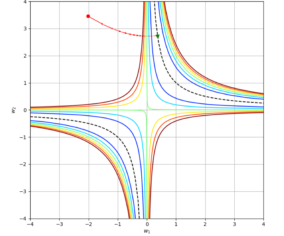
We can divide GD training with weight decay into two phases: (1) optimization and (2) regularization. During the first phase, the loss decreases until the trajectory gets into the WD-band. During the second phase, the loss LL can oscillate, but the trajectory stays inside the WD-band (Fig. 2(b)) and goes toward a flat minima area. The layer imbalance monotonically decreases:

d(wi2wj2)dt\displaystyle\frac{d(w_{i}^{2}-w_{j}^{2})}{dt} =4λ(((W1)W+μwi2)((W1)W+μwj2))=4λμ(wi2wj2)\displaystyle=-4\lambda\cdot\Big{(}\big{(}(W-1)W+\mu w_{i}^{2}\big{)}-\big{(}(W-1)W+\mu w_{j}^{2}\big{)}\Big{)}=-4\lambda\cdot\mu\cdot(w_{i}^{2}-w_{j}^{2})
Refer to caption
(a) Continuous GD
Refer to caption
(b) GD with weight decay
Refer to caption
(c) GD with noise augmentation
Figure 2: The training trajectories for (a) continuous GD, (b) GD with weight decay, and (c) GD with noise augmentation. The trajectory for continuous GD is a hyperbola: wi2(t)wj2(t)=w_{i}^{2}(t)-w_{j}^{2}(t)= const. The trajectories for GD with weight decay and noise augmentation have two parts: (1) optimization – the trajectory goes toward the minima manifold, and (2) regularization – the trajectory goes along minima manifold toward a flat area.

4.2 Training with noise augmentation

Bishop [3] showed that for shallow networks, training with noise is equivalent to Tikhonov regularization. We extend this result to DLNs.

Let’s augment the training data with noise: x~=x(1+η)\tilde{x}=x\cdot(1+\eta), where the noise η\eta has 00-mean and is bounded: |η|δ<12|\eta|\leq\delta<\frac{1}{2}. The DLN with noise augmentation can be written in the following form:

y~=w1wd(1+η)x\displaystyle\tilde{y}=w_{1}\cdots w_{d}\cdot(1+\eta)x (10)

This model also describes continuous dropout [11] when layer outputs hih_{i} are multiplied with the noise: h~i=(1+η)hi\tilde{h}_{i}=(1+\eta)\cdot h_{i}. This model can be also used for continuous drop-connect [8, 12] when the noise is applied to weights: w~i=(1+η)wi\tilde{w}_{i}=(1+\eta)\cdot w_{i}.

The GD with noise augmentation is described by the following stochastic DEs:

dwidt=λL~wi=2λ(1+η)(W(1+η)1)(W/wi)\displaystyle\frac{dw_{i}}{dt}=-\lambda\frac{\partial\tilde{L}}{\partial w_{i}}=-2\lambda\cdot(1+\eta)(W(1+\eta)-1)(W/w_{i})

Let’s consider loss dynamics:

dLdt=(Lwidwidt)=4λ(1+η)W2(1/wi2)(W1)(W(1+η)1)\displaystyle\frac{dL}{dt}=\sum\Big{(}\frac{\partial L}{\partial w_{i}}\cdot\frac{dw_{i}}{dt}\Big{)}=-4\lambda(1+\eta)W^{2}\big{(}\sum 1/w_{i}^{2}\big{)}(W-1)(W(1+\eta)-1)
=4λ(1+η)2W2(1/wi2)((W1)(W11+η))\displaystyle=-4\lambda(1+\eta)^{2}W^{2}\big{(}\sum 1/w_{i}^{2}\big{)}\cdot\Big{(}(W-1)(W-\frac{1}{1+\eta})\Big{)}

The loss decreases while the factor k=(W1)(W11+η)=(W1)(W1η1+η)>0k=(W-1)(W-\dfrac{1}{1+\eta})=(W-1)(W-1-\dfrac{\eta}{1+\eta})>0, outside of the noise band 1δ1+δ<W<1+δ1δ1-\dfrac{\delta}{1+\delta}<W<1+\dfrac{\delta}{1-\delta}. The training trajectory is the hyperbola wi2(t)wj2(t)=w_{i}^{2}(t)-w_{j}^{2}(t)= const. When the trajectory gets inside the noise band, it oscillates around the minima manifold, but the layer imbalance remains constant for continuous GD.

Consider now discrete GD with noise augmentation:

wi(t+1)=wi2λ(1+η)(W(1+η)1)(W/wi)\displaystyle w_{i}(t+1)=w_{i}-2\lambda(1+\eta)(W(1+\eta)-1)(W/w_{i}) (11)

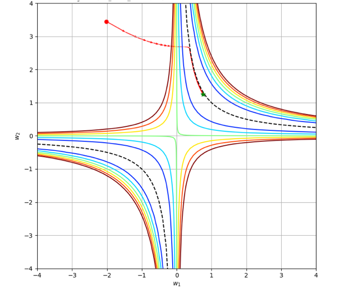
For discrete GD, noise augmentation works similarly to weight decay. Training has two phases: (1) optimization and (2) regularization (Fig. 2(c)). During the optimization phase, the loss decreases until the trajectory hits the noise band. Next, the trajectory oscillates inside the noise band, and the layer imbalance decreases. The noise variance σ2\sigma^{2} defines the band width, similarly to the weight decay μ\mu.

Theorem 4.1.

Consider discrete GD with noise augmentation (Eq. 11). Assume that the noise η\eta has 0-mean and is bounded: |η|<δ<12|\eta|<\delta<\dfrac{1}{2}. If we define the adaptive learning rate λ(𝐰)=12(23)511/wi2\lambda({\bm{w}})=\dfrac{1}{2}\Big{(}\dfrac{2}{3}\Big{)}^{5}\dfrac{1}{\sum 1/w_{i}^{2}}, then the layer imbalance monotonically decreases inside the noise band |W1|<δ|W-1|<\delta.

Proof.

Let’s estimate the layer imbalance:

wi2(t+1)wj2(t+1)\displaystyle w_{i}^{2}(t+1)-w_{j}^{2}(t+1)
=(wi2λ(1+η)(W(1+η)1)W/wi)2(wj2λ(1+η)(W(1+η)1)W/wj)2\displaystyle=\big{(}w_{i}-2\lambda(1+\eta)(W(1+\eta)-1)W/w_{i}\big{)}^{2}-\big{(}w_{j}-2\lambda(1+\eta)(W(1+\eta)-1)W/w_{j}\big{)}^{2}
=(wi2wj2)+4λ2(1+η)2(W(1+η)1)2(W2/wi2W2/wj2)\displaystyle=(w_{i}^{2}-w_{j}^{2})+4\lambda^{2}(1+\eta)^{2}(W(1+\eta)-1)^{2}\big{(}W^{2}/w_{i}^{2}-W^{2}/w_{j}^{2}\big{)}
=(wi2wj2)(14λ2(1+η)4(W11+η)2W2/(wiwj)2)\displaystyle=(w_{i}^{2}-w_{j}^{2})\cdot\Big{(}1-4\lambda^{2}(1+\eta)^{4}\big{(}W-\frac{1}{1+\eta}\big{)}^{2}W^{2}/(w_{i}w_{j})^{2}\Big{)}

On the one hand, the factor k=14λ2(1+η)4(W11+η)2W2/(wiwj)21k=1-4\lambda^{2}(1+\eta)^{4}\big{(}W-\dfrac{1}{1+\eta}\big{)}^{2}W^{2}/(w_{i}w_{j})^{2}\leq 1.

On the other hand:

k=14λ2(1+η)4(W11+η)2W2/(wiwj)2\displaystyle k=1-4\lambda^{2}(1+\eta)^{4}\big{(}W-\frac{1}{1+\eta}\big{)}^{2}W^{2}/(w_{i}w_{j})^{2}
1λ2(1+η)4(W11+η)2W2(1/wi2+1/wj2)2\displaystyle\geq 1-\lambda^{2}(1+\eta)^{4}\big{(}W-\frac{1}{1+\eta}\big{)}^{2}W^{2}(1/w_{i}^{2}+1/w_{j}^{2})^{2}
1λ2(1+η)4(W1+η1+η)2W2(i1/wi2)2\displaystyle\geq 1-\lambda^{2}(1+\eta)^{4}\big{(}W-1+\frac{\eta}{1+\eta}\big{)}^{2}W^{2}\big{(}\sum_{i}1/w_{i}^{2}\big{)}^{2}
1λ2(i1/wi2)2(1+δ)4(δ+δ1δ)2(1+δ)21λ2(i1/wi2)2(3/2)10\displaystyle\geq 1-\lambda^{2}\big{(}\sum_{i}1/w_{i}^{2}\big{)}^{2}\cdot(1+\delta)^{4}\big{(}\delta+\frac{\delta}{1-\delta}\big{)}^{2}(1+\delta)^{2}\geq 1-\lambda^{2}\big{(}\sum_{i}1/w_{i}^{2}\big{)}^{2}(3/2)^{10}

Taking λ=12(23)511/wi2\lambda=\dfrac{1}{2}\Big{(}\dfrac{2}{3}\Big{)}^{5}\dfrac{1}{\sum 1/w_{i}^{2}} makes 0<k10<k\leq 1, which proves that the layer imbalance decreases. ∎

Note. We can prove that the layer imbalance E[D]0E[D]\rightarrow 0 if we also assume that all layers are uniformly bounded |wi|<C|w_{i}|<C. This implies that there is ϵ>0\epsilon>0 such that for all 𝒘{\bm{w}} the adaptive learning rate λ(𝒘)>ϵ\lambda({\bm{w}})>\epsilon, and we can prove that the expectation E(k)<1E(k)<1:

E(k)=1E[4λ2(1+η)4(W11+η)2W2/(wiwj)2]\displaystyle E(k)=1-E\Big{[}4\lambda^{2}(1+\eta)^{4}\big{(}W-\frac{1}{1+\eta}\big{)}^{2}W^{2}/(w_{i}w_{j})^{2}\Big{]}
14λ2W2/(wiwj)2(1+σ2)2σ21+σ214λ214C4(1+σ2)σ21λ2σ2C4\displaystyle\leq 1-4\lambda^{2}W^{2}/(w_{i}w_{j})^{2}\cdot(1+\sigma^{2})^{2}\frac{\sigma^{2}}{1+\sigma^{2}}\leq 1-4\lambda^{2}\frac{1}{4C^{4}}\big{(}1+\sigma^{2}\big{)}\sigma^{2}\leq 1-\frac{\lambda^{2}\sigma^{2}}{C^{4}}

This proves that the layer imbalance D0D\rightarrow 0 with rate (1λ2σ2C4)\big{(}1-\dfrac{\lambda^{2}\sigma^{2}}{C^{4}}\big{)}.

5 SGD noise as implicit regularization

In this section, we show that SGD works as implicit noise regularization, and that the layer imbalance converges to 0. As before, we train a DLN y=Wxy=Wx with loss L(𝒘)=1N(Wxnyn)2L({\bm{w}})=\frac{1}{N}\sum(Wx_{n}-y_{n})^{2} on a normalized dataset with NN samples {xn,yn}\{x_{n},y_{n}\}:

xi=0;1Nxi2=1;yi=0;1Nxiyi=1.\displaystyle\sum x_{i}=0;\;\;\frac{1}{N}\sum x^{2}_{i}=1;\;\;\sum y_{i}=0;\;\;\frac{1}{N}\sum x_{i}y_{i}=1.

A stochastic gradient for a batch B¯\bar{B} with B<NB<N samples is:

LBwi=1|B|B¯2(Wxn2xnyn)W/wi=2(W(1BB¯xn2)(1BB¯xnyn))W/wi\displaystyle\frac{\partial L_{B}}{\partial w_{i}}=\frac{1}{|B|}\sum_{\bar{B}}2(Wx_{n}^{2}-x_{n}y_{n})W/w_{i}=2\Big{(}W(\frac{1}{B}\sum_{\bar{B}}x_{n}^{2})-(\frac{1}{B}\sum_{\bar{B}}x_{n}y_{n})\Big{)}W/w_{i}

If batch size BNB\rightarrow N, then terms B¯xn2Nxn2=1\sum_{\bar{B}}x_{n}^{2}\rightarrow\sum_{N}x_{n}^{2}=1 and B¯(xnyn)B¯(xnyn)=1\sum_{\bar{B}}(x_{n}y_{n})\rightarrow\sum_{\bar{B}}(x_{n}y_{n})=1.

So we can write the stochastic gradient in the following form:

LBwi=2(W(1+η1)(1+η2))W/wi=2(W1+(Wη1η2))W/wi\displaystyle\frac{\partial L_{B}}{\partial w_{i}}=2\Big{(}W(1+\eta_{1})-(1+\eta_{2})\Big{)}W/w_{i}=2\Big{(}W-1+(W\eta_{1}-\eta_{2})\Big{)}W/w_{i}

The factor (1+η1)(1+\eta_{1}) works as noise data augmentation, and the term η2\eta_{2} works as label noise. Both η1\eta_{1} and η2\eta_{2} have 0-mean. When loss is small, we can combine both components into one SGD noise term: η=Wη1η2\eta=W\eta_{1}-\eta_{2}. SGD noise η\eta has 0-mean. We assume that SGD noise variance depends on batch size in the following way: σ2(1B1N)\sigma^{2}\approx(\dfrac{1}{B}-\dfrac{1}{N}). The trajectory for continuous SGD is described by the stochastic DEs:

dwidt=λLBwi=2λ(W1+η)W/wi\displaystyle\frac{dw_{i}}{dt}=-\lambda\cdot\frac{\partial L_{B}}{\partial w_{i}}=-2\lambda\Big{(}W-1+\eta\Big{)}W/w_{i}

Let’s start with loss analysis:

dLdt=4λW2(1/wi2)(W1)(W1+η)\displaystyle\frac{dL}{dt}=-4\lambda W^{2}\big{(}\sum 1/w_{i}^{2}\big{)}\cdot(W-1)(W-1+\eta)

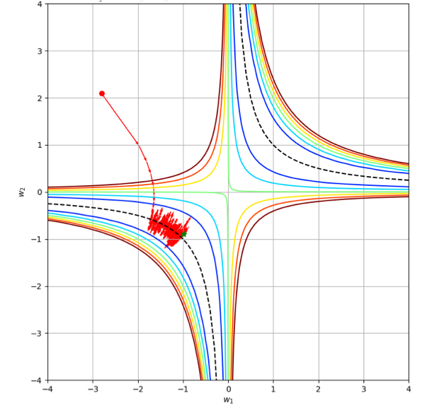
For continuous SGD, the loss decreases anywhere except in the SGD noise band: (W1)(W1+η)<0(W-1)(W-1+\eta)<0. The band width depends on BB: the smaller the batch, the wider the band. The SGD training consists of two parts. First, the loss decreases until the trajectory hits the SGD-noise band. Then the trajectory oscillates inside the noise band. The layer imbalance remains constant for continuous SGD.

Similarly to the noise augmentation, the layer imbalance decreases for discrete SGD:

wi(t+1)=wi2λ(W1+η)W/wi\displaystyle w_{i}(t+1)=w_{i}-2\lambda(W-1+\eta)W/w_{i} (12)
Theorem 5.1.

Consider discrete SGD (Eq. 12). Assume that |W1|<δ|W-1|<\delta, and that SGD noise satisfies |η|δ<1|\eta|\leq\delta<1. If we define the adaptive learning rate λ(𝐰)=12δ(1+δ)((1/wi2)\lambda({\bm{w}})=\dfrac{1}{2\delta(1+\delta)(\sum(1/w_{i}^{2})}, then the layer imbalance monotonically decreases.

Proof.

Let’s estimate the layer imbalance:

wi2(t+1)wj2(t+1)=(wi2λ(W1+η)W/wi)2(wj2λ(W1+η)W/wj)2\displaystyle w_{i}^{2}(t+1)-w_{j}^{2}(t+1)=\big{(}w_{i}-2\lambda(W-1+\eta)W/w_{i}\big{)}^{2}-\big{(}w_{j}-2\lambda(W-1+\eta)W/w_{j}\big{)}^{2}
=(wi2wj2)(14λ2(W1+η)2W2/(wiwj)2)\displaystyle=(w_{i}^{2}-w_{j}^{2})\cdot\Big{(}1-4\lambda^{2}(W-1+\eta)^{2}W^{2}/(w_{i}w_{j})^{2}\Big{)}

On the one hand, the factor k=14λ2(W1+η)2W2/(wiwj)21k=1-4\lambda^{2}(W-1+\eta)^{2}W^{2}/(w_{i}w_{j})^{2}\leq 1. On the other hand:

k\displaystyle k =14λ2(W1+η)2W2/(wiwj)212λ2(W1+η)2W2(1/wi2+1/wj2)2\displaystyle=1-4\lambda^{2}(W-1+\eta)^{2}W^{2}/(w_{i}w_{j})^{2}\geq 1-2\lambda^{2}(W-1+\eta)^{2}W^{2}\big{(}1/w_{i}^{2}+1/w_{j}^{2}\big{)}^{2}
14λ2W2(1/wi2)2((W1)2+η2)14λ2(1/wi2)2δ2(1+δ)2\displaystyle\geq 1-4\lambda^{2}W^{2}\big{(}\sum 1/w_{i}^{2}\big{)}^{2}\cdot((W-1)^{2}+\eta^{2})\geq 1-4\lambda^{2}\big{(}\sum 1/w_{i}^{2}\big{)}^{2}\cdot\delta^{2}(1+\delta)^{2}

Setting λ=12δ(1+δ)((1/wi2)\lambda=\dfrac{1}{2\delta(1+\delta)(\sum(1/w_{i}^{2})} makes 0<k10<k\leq 1, which completes the proof. ∎

The layer imbalance D0D\rightarrow 0 at a rate proportional to the variance of SGD noise. It was observed by Keskar et al. [7] that SGD training with a large batch leads to sharp solutions, which generalize worse than solutions obtained with a smaller batch. This fact directly follows from Theorem 5.1. The layer imbalance decreases at a rate O(1kλ2σ2)O(1-k\lambda^{2}\sigma^{2}). When a batch size increases, BNB\rightarrow N, the variance of SGD-noise decreases as (1B1N){\approx(\dfrac{1}{B}-\dfrac{1}{N})}. One can compensate for smaller SGD noise with additional generalization: data augmentation, weight decay, dropout, etc.

6 Discussion

In this work, we explore dynamics for gradient descent training of deep linear networks. Using the layer imbalance metric, we analyze how regularization methods such as L2L_{2}-regularization, noise data augmentation, dropout, etc, affect training dynamics. We show that for all these methods the training has two distinct phases: optimization and regularization. During the optimization phase, the training trajectory goes from an initial point toward minima manifold, and loss monotonically decreases. During the regularization phase, the trajectory goes along minima manifold toward flat minima, and the layer imbalance monotonically decreases. We derive an analytical proof that noise augmentation and continuous dropout work similarly to L2L_{2}-regularization. Finally, we show that SGD behaves in the same way as gradient descent with noise regularization.

This work provides an analysis of regularization for scalar linear networks. We leave the question of how regularization works for over-parameterized nonlinear networks for future research. The work also gives a few interesting insights into training dynamics, which can lead to new algorithms for large batch training, new learning rate policies, etc.

Acknowledgments

We would like to thank Vitaly Lavrukhin, Nadav Cohen and Daniel Soudry for the valuable feedback.

References

  • Arora et al. [2019] S. Arora, N. Golowich, N. Cohen, and W. Hu. A convergence analysis of gradient descent for deep linear neural networks. In ICLR, 2019.
  • Baldi and Hornik [1989] P. Baldi and K. Hornik. Neural networks and principal component analysis: Learning from examples without local minima. In Neural Networks 2.1, page 53–58, 1989.
  • Bishop [1995] C. M. Bishop. Training with noise is equivalent to Tikhonov regularization. Neural Computation, 7:108–116., 1995.
  • Dinh et al. [2017] Laurent Dinh, Razvan Pascanu, Samy Bengio, and Yoshua Bengio. Sharp minima can generalize for deep nets. In ICML, 2017.
  • Hochreiter and Schmidhuber [1994a] S. Hochreiter and J. Schmidhuber. Simplifying neural nets by discovering flat minima. In NIPS, 1994a.
  • Hochreiter and Schmidhuber [1994b] S. Hochreiter and J. Schmidhuber. Flat minima search for discovering simple nets, technical report fki-200-94. Technical report, Fakultat fur Informatik, H2, Technische Universitat Munchen, 1994b.
  • Keskar et al. [2016] N. S. Keskar, D. Mudigere, J. Nocedal, M. Smelyanskiy, and P. T. P. Tang. On large-batch training for deep learning: generalization gap and sharp minima. In ICLR, 2016.
  • Kingma et al. [2015] D. Kingma, T. Salimans, and M. Welling. Variational dropout and the local reparameterization trick. In NIPS, 2015.
  • Neyshabur et al. [2015] Behnam Neyshabur, Ruslan Salakhutdinov, and Nathan Srebro. Path-sgd: Path-normalized optimization in deep neural networks. In NIPS, page 2422–2430, 2015.
  • Saxe et al. [2013] Andrew M. Saxe, James L. McClelland, and Surya Ganguli. Exact solutions to the nonlinear dynamics of learning in deep linear neural network. In ICLR, 2013.
  • Srivastava et al. [2014] N. Srivastava, G. E. Hinton, A. Krizhevsky, I. Sutskever, and R. Salakhutdinov. Dropout: a simple way to prevent neural networks from overfitting. Journal of Machine Learning Research, 2014.
  • Wan et al. [2013] Li Wan, Matthew Zeiler, Sixin Zhang, Yann Le Cun, and Rob Fergus. Regularization of neural networks using dropconnect. In ICML, 2013.