On soft factors and transmutation operators

The bi-adjoint scalar (BAS) amplitudes describe scattering of massless scalars, with cubic interactions. In this paper, we are interested in the double ordered partial BAS amplitudes at the tree level. Each $n$-point double ordered amplitude ${\cal A}_{\rm BAS}(\vec{\boldsymbol{\sigma}}|\vec{\boldsymbol{\sigma}}^{\prime}_{n})$ carries two orderings encoded as $\vec{\boldsymbol{\sigma}}$ and $\vec{\boldsymbol{\sigma}}^{\prime}_{n}$, and is simultaneously planar with respect to both two orderings. Here we give a $5$-point example. The first diagram in Figure.1 contributes to the amplitude ${\cal A}_{\rm BAS}(1,2,3,4,5|1,4,2,3,5)$, since it is compatible with both two orderings $1,2,3,4,5$ and $1,4,2,3,5$. Meanwhile, the second diagram violates the ordering $1,4,2,3,5$, thus is forbidden. One can verify that the first diagram in Figure.1 is the only candidate satisfies two orderings simultaneously, thus the amplitude ${\cal A}_{\rm BAS}(1,2,3,4,5|1,4,2,3,5)$ reads

up to an overall sign. Here the Mandelstam variable $s_{i\cdots j}$ is defined as

where $k_{a}$ is the momentum carried by the external leg $a$.

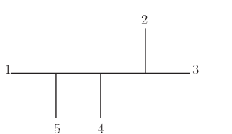
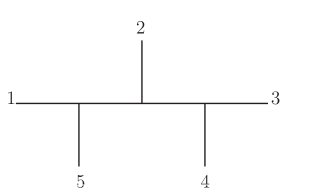
In double ordered BAS amplitudes, each interaction vertex features antisymmetry for lines attached to it. In other words, swamping two lines $a$ and $b$ at a vertex creates a $-$ sign, therefore BAS amplitudes with different orderings carry different overall $\pm$ sign. To simplify the description of soft behavior, we choose the overall sign to be $+$ if two orderings carried by the BAS amplitude are the same. For example, the amplitude ${\cal A}_{\rm BAS}(1,2,3,4|1,2,3,4)$ carries the overall sign $+$ under our convention. The sign for amplitudes with two different orderings can be generated from the above reference one by counting flippings, via the diagrammatic technic proposed in Cachazo:2013iea .

Due to the definition of tree BAS amplitudes introduced above, it is direct to observe the leading soft behavior of BAS amplitude ${\cal A}_{\rm BAS}(1,\cdots,n|\vec{\boldsymbol{\sigma}}_{n})$. Take the external scalar $i$ to be the soft particle, with $k_{i}^{\mu}\sim\tau k_{i}^{\mu}$ and $\tau\to 0$, then the propagators $1/s_{i(i-1)}$ and $1/s_{i(i+1)}$ become divergent in such soft limit, therefore

Throughout this paper, we use the superscript $(a)_{i}$ to denote the contribution at the $a^{\rm th}$ order, with the particle $i$ taken to be soft. In the above, the leading soft factor $S^{(0)_{i}}_{s}$ is given by

where the symbol $\delta_{ij}$ is determined by positions of $i$ and $j$ in the ordering $\vec{\boldsymbol{\sigma}}_{n}$. If $i$, $j$ are not adjacent to each other, $\delta_{ij}=0$. If $i$ and $j$ are two adjacent elements, we have $\delta_{ij}=1$ for $i\prec j$, $\delta_{ij}=-1$ for $j\prec i$. The notation $a\prec b$ for a given permutation including elements $a$, $b$ means the position of $a$ is on the left side of the position of $b$.

The higher order soft behaviors can also be analysed by considering contributions from allowed Feynman diagrams. However, suppose we formally express them as

the soft factors $S^{(a)_{i}}_{s}$ with $a\geq 1$ do not satisfy the universality. For example, the $4$-point BAS amplitudes only have the leading order term, while the higher-point amplitudes receives contribution from higher orders. In this sense, for tree BAS amplitudes under consideration, the expected universal soft factor only exist at the leading order.

The transmutation operators proposed by Cheung, Shen and Wen connects tree amplitudes of different theories together, by transmuting amplitudes of one theory to those of another Cheung:2017ems . In this paper, we only use the combinatorial operator ${\cal T}[1,\cdots,n]$, which turns GR amplitudes to ordered YM amplitudes, and also transmutes YM amplitudes to double ordered BAS amplitudes, namely,

In the above, ${\boldsymbol{h}}_{n}$ stands for the unordered set of $n$ external gravitons, and $\vec{\boldsymbol{\sigma}}_{n}$ labels the ordered set of $n$ external gluons. The polarization tensor of each graviton is decomposed as $\varepsilon_{p}^{\mu\nu}=\epsilon_{p}^{\mu}\widetilde{\epsilon}_{p}^{\nu}$, where $\epsilon_{p}$ and $\widetilde{\epsilon}_{p}$ with $p\in\{1,\cdots,n\}$ are two sectors of polarization vectors. The operator $\widetilde{\cal T}[1,\cdots,n]$ is defined for polarization vectors $\widetilde{\epsilon}_{p}$ (as will be explicitly explained soon), transmutes the unordered GR amplitude ${\cal A}_{\rm GR}(\boldsymbol{h}_{n})$ to the YM amplitude ${\cal A}_{\rm YM}(1,\cdots,n)$ with ordering $1,\cdots,n$, and the external gluons carry polarization vectors $\epsilon_{p}$. The operator ${\cal T}[1,\cdots,n]$ is defined for polarization vectors $\epsilon_{p}$, transmutes the ordered YM amplitude ${\cal A}_{\rm YM}(\vec{\boldsymbol{\sigma}}_{n})$ to the double ordered BAS amplitude ${\cal A}_{\rm BAS}(1,\cdots,n|\vec{\boldsymbol{\sigma}}_{n})$ for scalars without any polarization. Notice that the relation in (8) which turns GR amplitude to YM one only makes sense for the extended gravity theory that Einstein gravity is coupled to a $2$-form and dilaton field.

One of the explicit forms for the combinatorial operator ${\cal T}[1,\cdots,n]$ is given by

where the insertion operator ${\cal I}_{bac}$ is defined as

The above ${\cal T}[1,\cdots,n]$ is defined for polarization vectors $\epsilon_{p}$. The dual operator $\widetilde{\cal T}[1,\cdots,n]$, defined for polarization vectors $\widetilde{\epsilon}_{p}$, can be obtained from ${\cal T}[1,\cdots,n]$ by replacing all $\epsilon_{p}$ with $\widetilde{\epsilon}_{p}$. As proved in Zhou:2018wvn ; Bollmann:2018edb , the effect of insertion operator ${\cal I}_{bac}$ is to reduce the spin of particle $a$ by $1$, and insert it between $b$ and $c$ in the ordering. According to the above interpretation for insertion operator, the effect of the operator ${\cal T}[1,\cdots,n]$ in (9) can be understood as,

• •

  Generating two endpoints $1$ and $n$ of the ordering.

• •

  Inserting the leg $2$ between $1$ and $n$.

• •

  Inserting the leg $3$ between $2$ and $n$.

• •

  Repeating the above procedure to insert other legs in turn, until the full ordering $1,\cdots,n$ is completed.

The above steps exhibit the process for generating the full ordering. Notice that we assume the order of performing differentials in (9) to be from right to left. However, since all insertion operators in (9) are algebraically commutative, we can rearrange the order as ${\cal I}_{(n-2)(n-1)n}{\cal I}_{(n-3)(n-2)n}\cdots{\cal I}_{23n}{\cal I}_{12n}$, and interpret the effects of them in the above way.

To create any desired ordering $\vec{\boldsymbol{\sigma}}_{n}$, the corresponding formula of combinatorial operator ${\cal T}[\vec{\boldsymbol{\sigma}}_{n}]$ is not unique, due to the interpretation for the insertion operator ${\cal I}_{bac}$. For instance, to generate the ordering $1,2,3,4$ one can chose

which realizes the goal as

• •

  Generating two endpoints $1$ and $4$.

• •

  Inserting the leg $2$ between $1$ and $4$.

• •

  Inserting the leg $3$ between $2$ and $4$.

However, the different choice

is also correct, this operator generates the ordering $1,2,3,4$ as

• •

  Generating two endpoints $1$ and $4$.

• •

  Inserting the leg $3$ between $1$ and $4$.

• •

  Inserting the leg $2$ between $1$ and $3$.

Such freedom for choosing the combinatorial operator ${\cal T}[1,\cdots,n]$ will play the crucial role in subsequent sections.

The analogous operator ${\cal T}[\vec{\boldsymbol{\sigma}}_{m}]$, where $\vec{\boldsymbol{\sigma}}_{m}$ is the ordering among $m$ elements in the complete set $\{1,\cdots,n\}$, with $m<n$, also leads to the meaningful interpretation. For instance, one can define ${\cal T}[2,3,4]={\cal I}_{234}\partial_{\epsilon_{2}\cdot\epsilon_{4}}$. When acting on the $4$-point YM amplitude ${\cal A}_{\rm YM}(\vec{\boldsymbol{\sigma}}_{4})$ with external gluons encoded as $\{1,2,3,4\}$, the above operator ${\cal T}[2,3,4]$ turns gluons in the set $\{2,3,4\}$ to scalars, and generates the ordering $2,3,4$. The resulted amplitude ${\cal A}_{\rm YMS}(2,3,4;1|\vec{\boldsymbol{\sigma}}_{4})$ is known as the Yang-Mills-scalar (YMS) amplitude that the gluon $1$ interacts with BAS scalars in $\{2,3,4\}$. Similarly, the operators $\widetilde{\cal T}[\vec{\boldsymbol{\sigma}}_{m}]$ with $m<n$ transmutes GR amplitudes to Einstein-Yang-Mills (EYM) amplitudes those gravitons couple to gluons.

Consider the soft behavior of any $n$-point amplitude ${\cal A}_{n}$, with $k_{i}\to\tau k_{i}$, $\tau\to 0$. One can always expand the full amplitude as in (2), to acquire the formal factorization behavior ${\cal A}^{(a)_{i}}_{n}=S^{(a)_{i}}\,{\cal A}_{n-1}$ at any order. Since such formula is not the physically expected factorization, we need to impose appropriate constraints on soft factors.

The first important constraint is the universality, i.e., the expression of the soft factor is independent on the number of external legs. For $4$-point amplitudes, all allowed propagators have the form $1/s_{ij}$ where $i$ is the soft particle under consideration, thus the denominator of each term behaves as $\tau s_{ij}$ in the soft limit. Therefore, for the $4$-point case, the formula of soft factor at $a^{\rm th}$ order is restricted to

where the summation is over all $j$ those $1/s_{ij}$ contribute to ${\cal A}_{n}$. Then the universality requires the formula of soft factors in (13) should also be satisfied for higher-point cases. It is impossible to extended the formula (13) to incorporate propagators like $1/s_{ijk}$ from multi-particle channels without breaking the universality, since these propagators do not proportional to $1/\tau$ thus can not be on an equal footing with $1/s_{ij}$. If the formula (13) for arbitrary number of external particles does not hold at the $a^{\rm th}$ order, then we say the universal soft factor does not exist at this order, since the independence on the number of external legs is violated.

For the YM case under consideration in this section, the numerator $N^{(a)}_{ij}(\epsilon_{i},k_{i},k_{\ell})$ depends on $\epsilon_{i}$, $k_{i}$ for the soft gluon, and $k_{\ell}$ carried by other external gluons, but is independent of any $\epsilon_{\ell}$ with $\ell\neq i$, since both ${\cal A}^{(a)_{i}}_{\rm YM}(\vec{\boldsymbol{\sigma}}_{n})$ and ${\cal A}_{\rm YM}(\vec{\boldsymbol{\sigma}}_{n}\setminus i)$ are linear on each $\epsilon_{\ell}$. We allow each soft factor to be an operator, acts on $(n-1)$-point amplitudes, then the independence on $\epsilon_{\ell}$ should be understood as that the effect of acting operator $N^{(a)}_{ij}(\epsilon_{i},k_{i},k_{\ell})$ doe not break the linearity on $\epsilon_{\ell}$.

Furthermore, for the gluons of YM theory, we can extended the universality of soft behavior to a stronger version: the soft factors of pure YM amplitudes also holds for Yang-Mills-scalar (YMS) amplitudes in which gluons interact with BAS scalars. The reason is, the $3$-point YMS amplitude with two external scalars $1,3$ and one external gluon $2$, is related to the $3$-point YM amplitude via the operator $\partial_{\epsilon_{1}\cdot\epsilon_{3}}$ introduced in section 2.2. The differential $\partial_{\epsilon_{1}\cdot\epsilon_{3}}$ is equivalent to the dimensional reduction, namely, consider the $(d+1)$-dimensional space-time, let the nonzero components of $\epsilon_{1}$ and $\epsilon_{3}$ to be in the extra dimension, and keep $\epsilon_{2}$ and all $k_{p}$ with $p\in\{1,2,3\}$ to be in the ordinary $d$-dimensional space-time. From $d$-dimensional point of view, $1$ and $3$ behaves as two scalars while $2$ behaves as a gluon. However, from the $(d+1)$-dimensional perspective, the $d$-dimensional scalar-scalar-gluon and gluon-gluon-gluon vertices are exactly the same interaction. Based on the above reason, it is nature to generalize the universality of gluon soft behaviors to the YMS case. Such extended universality will be useful in subsequent works.

Now we discuss the constraints from gauge invariance. To make the discussion clear, let us define the Ward identity operator as

where the summation is over all Lorentz vectors $v^{\mu}$. Each numerator $N^{(a)}_{ij}(\epsilon_{i},k_{i},k_{\ell})$ in (13) should be consistent with gauge invariance for polarizations carried by external gluons, i.e.,

In the above, the first equality holds because the $(n-1)$-point amplitude ${\cal A}_{\rm YM}(\vec{\boldsymbol{\sigma}}_{n}\setminus i)$ in independent on $\epsilon_{i}$ when $q=i$, and states the gauge invariance of the amplitude ${\cal A}_{\rm YM}(\vec{\boldsymbol{\sigma}}_{n}\setminus i)$ when $q\neq i$. The second is based on the gauge invariance of ${\cal A}_{\rm YM}(\vec{\boldsymbol{\sigma}}_{n})$ and the definition ${\cal A}^{(a)_{i}}_{\rm YM}(\vec{\boldsymbol{\sigma}}_{n})=S^{(a)_{i}}_{g}\,{\cal A}_{\rm YM}(\vec{\boldsymbol{\sigma}}_{n}\setminus i)$. Thus, we conclude the commutativity $[{\cal W}_{q},S^{(a)_{i}}_{g}]=0$, due to the relation in (15).

Such commutativity requires the soft operator $S^{(a)_{i}}_{g}$ to have the form

where each $P^{(a)}_{ij;r}(\epsilon_{i},k_{i},k_{\ell})$ is a polynomial of Lorentz invariants, while each ${\cal O}^{(a)}_{ij;r}$ is an operator. The summation over integers $r$ means we allow more than one operators contribute to the numerator $N^{(a)}_{ij}(\epsilon_{i},k_{i},k_{\ell})$, albeit all cases which will be encountered in this note are those $k=1$. The operator ${\cal O}^{(a)}_{ij;r}$ satisfies that when acting on any Lorentz invariant $k_{p}\cdot v$, the linearity on $k_{p}$ is kept, due to the following reason. The operator $S^{(a)_{i}}_{g}$ transmutes the Lorentz invariant $\epsilon_{p}\cdot v$ with $p\neq i$ as follows

without breaking the linearity on $\epsilon_{p}$, as discussed previously. Here we have replaced the Lorentz vector $v^{\mu}$ by new ones $(v^{\prime}_{j;r})^{\mu}$, to reflect the action of ${\cal O}^{(a)}_{ij;r}$. Therefore, we have

Then the commutation relation $[{\cal W}_{p},S^{(a)_{i}}_{g}]=0$ leads to

which means the operators ${\cal O}^{(a)}_{ij;r}$ do not affect the linearity on $k_{p}$.

With the expected formula (16) and the property of ${\cal O}^{(a)}_{ij;r}$ displayed above, now we are ready to study the existence of soft factors at each order.

In this subsection, we use transmutation operators to investigate whether the leading order soft behavior of the YM amplitude ${\cal A}_{\rm YM}(\vec{\boldsymbol{\sigma}}_{n})$ can be represented as the factorized formula

where the leading soft factor $S^{(0)_{i}}_{g}$ satisfies the required form in (16).

We chose the combinatorial transmutation operator ${\cal T}[1,\cdots,n]$ to be

which creates the ordering $1,\cdots,n$ as follows:

• •

  Generating two endpoints $1$ and $n$ of the ordering.

• •

  Inserting legs $a$ with $a\in\{2,\cdots,i-1\}$ between $1$ and $n$.

• •

  Inserting the leg $(i+1)$ between $(i-1)$ and $n$.

• •

  Inserting legs $a$ with $a\in\{i+2,\cdots,n-1\}$ between $(i+1)$ and $n$.

• •

  Inserting the leg $i$ between $(i-1)$ and $(i+1)$.

In the operator (21), all $\partial_{\epsilon_{a}\cdot k_{n}}$ in ${\cal I}_{(a-1)an}$ are removed, since all $k_{n}$ in the amplitude are eliminated by using momentum conservation. It is straightforward to recognize that

where the operator ${\cal T}[1,\cdots,i-1,i+1,\cdots,n]$ transmutes the $n$-point YM amplitude to YMS one as follows

Now we use the operator chosen in (21) to link the soft behaviors of gluons and BAS scalars together. We can expand the BAS and YM amplitudes by $\tau$, then the transmutation relation in (8) reads

Since the operator ${\cal T}_{0}[1,\cdots,n]$ in (21) does not include any $\partial_{\epsilon_{p}\cdot k_{i}}$, it is independent of the soft parameter $\tau$. Consequently, we have

holds at any order.

At the leading order, one can substitute the soft behavior of BAS amplitude given in (5) and (6), to obtain

Suppose ${\cal A}^{(0)_{i}}_{\rm YM}(\vec{\boldsymbol{\sigma}}_{n})$ satisfies the factorized formula (20), then we have

where the second equality uses the observation

based on the transmutation relation (23). The third uses

which is indicated by the universality of soft behavior, namely, the formula (29) holds as long as (20) holds, with exactly the same soft factor. Substituting (27) into (26), we find the equations

hold for any $i\in\{2,\cdots,n-1\}$ (for $i=n-1$, the operator $\partial_{\epsilon_{i}\cdot k_{i+1}}$ in ${\cal I}_{(i-1)i(i+1)}$ should be removed, since we have eliminated all $k_{n}$ in the amplitude via momentum conservation).

The unique solution to equations (30) for all $i\in\{2,\cdots,n-1\}$ is found to be

Notice that for $i=n-1$, the corresponding equation

is not sufficient to determine the term $\delta_{ni}(\epsilon_{i}\cdot k_{n})/s_{in}$ in the solution (31). This term is fixed by considering the gauge invariance for the polarization $\epsilon_{i}$. Start from the the ansatz

the gauge invariance indicates

then the relation $\sum_{k\neq i}\delta_{ki}=0$ together with the linearity on $\epsilon_{i}$ fix $X$ to be $\delta_{ni}(\epsilon_{i}\cdot n)$. Comparing with the expected formula (16), we see that the polynomial is $P^{(0)}_{ij;1}(\epsilon_{i},k_{i},k_{\ell})=\delta_{ji}(\epsilon_{i}\cdot k_{j})$, the operator is the identity operator ${\cal O}^{(0)}_{ij;1}=\boldsymbol{1}$. The symbol $\delta_{ji}$ requires the effective legs $j$ to be those adjacent to $i$ in the ordering $\vec{\boldsymbol{\sigma}}_{n}$, thus ensured that the summation is for all $j$ those the corresponding $1/s_{ij}$ contribute to the amplitude.

It is worth to point out that the result in (27) also implies the commutativity

due to the soft behavior (20) and the transmutation relation

In general, the above interpretation is not correct for the operator ${\cal T}[1,\cdots,i-1,i+1,\cdots,n]$ defined in (22), since momenta carried by gluons in the set $\{1,\cdots,n\}\setminus i$ violate momentum conservation. However, such interpretation makes sense in the soft limit $\tau\to 0$. The commutativity in (35) can be generalized to arbitrary order as

if the soft factor satisfies the requirement in (16) exisit at the $a^{\rm th}$ order. The general commutation relation

will be useful in subsequent subsections.

In this subsection, we continue to study the soft behavior of YM amplitudes at the sub-leading order. The relation (72) also links the soft behaviors of YM and BAS amplitudes at the sub-leading order. However, since the factorized formula for BAS amplitudes is lacked, one can not repeat the manipulation in the previous subsection 3.2, to solve the sub-leading YM soft factor from the BAS one. Therefore, the operator ${\cal T}_{0}[1,\cdots,n]$ chosen in (21) and the relation (72) are not effective for the current case. The above obstacle motivates us to chose new operator ${\cal T}_{1}[1,\cdots,n]$ which connects the sub-leading term of the YM side and the leading term of the BAS side together.

The new operator ${\cal T}_{1}[1,\cdots,n]$ is chosen to be that in (9). Based on the assumption that all $k_{n}$ in amplitudes are removed via momentum conservation, we can remove all $\partial_{\epsilon_{p}\cdot k_{n}}$ in the insertions operators ${\cal I}_{(a-1)an}$ to obtain

In the soft limit, the operator (39) transmutes the expanded YM amplitude to expanded BAS amplitude as follows

Using the leading soft factor (31), it is direct to see that the operator ${\cal T}_{1}[1,\cdots,n]$ annihilates the leading order YM term ${\cal A}^{(0)_{i}}_{\rm YM}(\vec{\boldsymbol{\sigma}}_{n})$, since ${\cal T}_{1}[1,\cdots,n]$ involves the differential operator $\partial_{\epsilon_{i+1}\cdot k_{i}}$, while ${\cal A}^{(0)_{i}}_{\rm YM}(\vec{\boldsymbol{\sigma}}_{n})$ is independent of $k_{i}$. The operator $\partial_{\epsilon_{i+1}\cdot k_{i}}$ carries the parameter $1/\tau$ when $k_{i}\to\tau k_{i}$, therefore, the operator ${\cal T}_{1}[1,\cdots,n]$ transmutes the sub-leading YM term ${\cal A}^{(1)_{i}}_{\rm YM}(\vec{\boldsymbol{\sigma}}_{n})$ to the leading BAS term ${\cal A}^{(0)_{i}}_{\rm BAS}(1,\cdots,n|\vec{\boldsymbol{\sigma}}_{n})$. Thus, suppose the sub-leading soft behavior of YM amplitude satisfies the factorization

one can use the transmutation relation based on ${\cal T}_{1}[1,\cdots,n]$, to solve the soft factor $S^{(1)_{i}}_{g}$ from the leading soft behavior of BAS amplitude.

Based on above discussions, we can find the following relation for the assumed sub-leading soft factor $S^{(1)_{i}}_{g}$,

References

• (1) F. E. Low, Bremsstrahlung of very low-energy quanta in elementary particle collisions, Phys. Rev. 110 (1958) 974–977.
• (2) S. Weinberg, Infrared photons and gravitons, Phys. Rev. 140 (1965) B516–B524.
• (3) F. Cachazo and A. Strominger, Evidence for a New Soft Graviton Theorem, arXiv:1404.4091.
• (4) E. Casali, Soft sub-leading divergences in Yang-Mills amplitudes, JHEP 08 (2014) 077, [arXiv:1404.5551].
• (5) B. U. W. Schwab and A. Volovich, Subleading Soft Theorem in Arbitrary Dimensions from Scattering Equations, Phys. Rev. Lett. 113 (2014), no. 10 101601, [arXiv:1404.7749].
• (6) N. Afkhami-Jeddi, Soft Graviton Theorem in Arbitrary Dimensions, arXiv:1405.3533.
• (7) M. Zlotnikov, Sub-sub-leading soft-graviton theorem in arbitrary dimension, JHEP 10 (2014) 148, [arXiv:1407.5936].
• (8) R. Britto, F. Cachazo, and B. Feng, New recursion relations for tree amplitudes of gluons, Nucl. Phys. B 715 (2005) 499–522, [hep-th/0412308].
• (9) R. Britto, F. Cachazo, B. Feng, and E. Witten, Direct proof of tree-level recursion relation in Yang-Mills theory, Phys. Rev. Lett. 94 (2005) 181602, [hep-th/0501052].
• (10) F. Cachazo, S. He, and E. Y. Yuan, Scattering equations and Kawai-Lewellen-Tye orthogonality, Phys. Rev. D90 (2014), no. 6 065001, [arXiv:1306.6575].
• (11) F. Cachazo, S. He, and E. Y. Yuan, Scattering of Massless Particles in Arbitrary Dimensions, Phys. Rev. Lett. 113 (2014), no. 17 171601, [arXiv:1307.2199].
• (12) F. Cachazo, S. He, and E. Y. Yuan, Scattering of Massless Particles: Scalars, Gluons and Gravitons, JHEP 07 (2014) 033, [arXiv:1309.0885].
• (13) F. Cachazo, S. He, and E. Y. Yuan, Einstein-Yang-Mills Scattering Amplitudes From Scattering Equations, JHEP 01 (2015) 121, [arXiv:1409.8256].
• (14) F. Cachazo, S. He, and E. Y. Yuan, Scattering Equations and Matrices: From Einstein To Yang-Mills, DBI and NLSM, JHEP 07 (2015) 149, [arXiv:1412.3479].
• (15) Z. Bern, S. Davies, and J. Nohle, On Loop Corrections to Subleading Soft Behavior of Gluons and Gravitons, Phys. Rev. D 90 (2014), no. 8 085015, [arXiv:1405.1015].
• (16) S. He, Y.-t. Huang, and C. Wen, Loop Corrections to Soft Theorems in Gauge Theories and Gravity, JHEP 12 (2014) 115, [arXiv:1405.1410].
• (17) F. Cachazo and E. Y. Yuan, Are Soft Theorems Renormalized?, arXiv:1405.3413.
• (18) M. Bianchi, S. He, Y.-t. Huang, and C. Wen, More on Soft Theorems: Trees, Loops and Strings, Phys. Rev. D 92 (2015), no. 6 065022, [arXiv:1406.5155].
• (19) A. Sen, Subleading Soft Graviton Theorem for Loop Amplitudes, JHEP 11 (2017) 123, [arXiv:1703.00024].
• (20) D. Nguyen, M. Spradlin, A. Volovich, and C. Wen, The Tree Formula for MHV Graviton Amplitudes, JHEP 07 (2010) 045, [arXiv:0907.2276].
• (21) C. Boucher-Veronneau and A. J. Larkoski, Constructing Amplitudes from Their Soft Limits, JHEP 09 (2011) 130, [arXiv:1108.5385].
• (22) L. Rodina, Scattering Amplitudes from Soft Theorems and Infrared Behavior, Phys. Rev. Lett. 122 (2019), no. 7 071601, [arXiv:1807.09738].
• (23) S. Ma, R. Dong, and Y.-J. Du, Constructing EYM amplitudes by inverse soft limit, JHEP 05 (2023) 196, [arXiv:2211.10047].
• (24) C. Cheung, K. Kampf, J. Novotny, and J. Trnka, Effective Field Theories from Soft Limits of Scattering Amplitudes, Phys. Rev. Lett. 114 (2015), no. 22 221602, [arXiv:1412.4095].
• (25) C. Cheung, K. Kampf, J. Novotny, C.-H. Shen, and J. Trnka, On-Shell Recursion Relations for Effective Field Theories, Phys. Rev. Lett. 116 (2016), no. 4 041601.
• (26) H. Luo and C. Wen, Recursion relations from soft theorems, JHEP 03 (2016) 088, [arXiv:1512.06801].
• (27) H. Elvang, M. Hadjiantonis, C. R. T. Jones, and S. Paranjape, Soft Bootstrap and Supersymmetry, JHEP 01 (2019) 195, [arXiv:1806.06079].
• (28) K. Zhou, Tree level amplitudes from soft theorems, JHEP 03 (2023) 021, [arXiv:2212.12892].
• (29) F.-S. Wei and K. Zhou, Expanding single-trace YMS amplitudes with gauge-invariant coefficients, Eur. Phys. J. C 84 (2024), no. 1 29, [arXiv:2306.14774].
• (30) C. Hu and K. Zhou, Recursive construction for expansions of tree Yang–Mills amplitudes from soft theorem, Eur. Phys. J. C 84 (2024), no. 3 221, [arXiv:2311.03112].
• (31) Y.-J. Du and K. Zhou, Multi-trace YMS amplitudes from soft behavior, JHEP 03 (2024) 081, [arXiv:2401.03879].
• (32) C. Cheung, C.-H. Shen, and C. Wen, Unifying Relations for Scattering Amplitudes, JHEP 02 (2018) 095, [arXiv:1705.03025].
• (33) K. Zhou and B. Feng, Note on differential operators, CHY integrands, and unifying relations for amplitudes, JHEP 09 (2018) 160, [arXiv:1808.06835].
• (34) M. Bollmann and L. Ferro, Transmuting CHY formulae, JHEP 01 (2019) 180, [arXiv:1808.07451].
• (35) A. Strominger, On BMS Invariance of Gravitational Scattering, JHEP 07 (2014) 152, [arXiv:1312.2229].
• (36) T. He, V. Lysov, P. Mitra, and A. Strominger, BMS supertranslations and Weinberg’s soft graviton theorem, JHEP 05 (2015) 151, [arXiv:1401.7026].